1. The document contains 20 problems related to reliability engineering and design for reliability. The problems cover topics like calculating service life, tolerance analysis, interference fits, system reliability, and reliability of components.
2. Solutions to the problems are provided in the solutions manual. The problems get progressively more complex and involve reliability concepts like Weibull distribution, fatigue life, mean time between failures, and fault tree analysis.
3. The document is from a textbook on advanced engineering design with a focus on designing for reliability. It provides real-world examples and problems to help students learn reliability engineering techniques.

![Design for lifetime performance and reliability 3
Problems Chapter 1
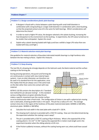
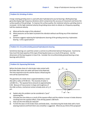
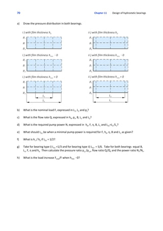
Problem 1.1: L10 service life
Consider a quantity of 10 components that all fail within a year of service. Calculate the L10 service life
with 90% reliability and 10% failure probability assuming a normal failure distribution.
Months 1 2 3 4 5 6 7 8 9 10 11 12
Failures 0 0 0 0 0 1 2 4 2 1 0 0
Problem 1.2: Tolerance field
The diameter of a batch of shafts is normally distributed
with 99.7% of the shafts within the tolerance field
20±0.2mm. Then 95% of the shafts will have a diameter
within a tolerance field of 20 mm ±A mm.
a) What is A?
b) What is the coefficient of variation CV’?
CV’ is defined as the maximum deviation of the mean
divided by the mean.
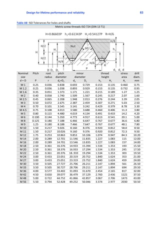
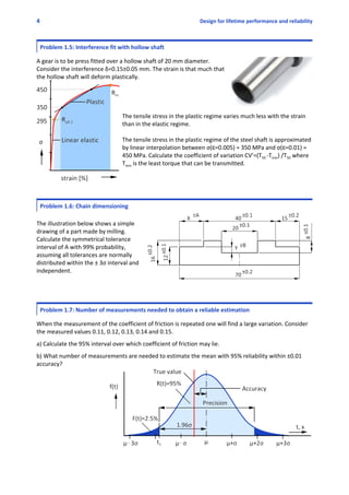
Problem 1.3: Driving torque interference fit
An interference fit is realized with 20 H7/r6 hole/shaft tolerances. The
dimensions of the components are assumed to be normally distributed.
The standard deviation is calculated from the assumption that the
tolerance interval is a ±3σ interval. Linear elastic deformation is to be
considered which implies the torque that can be transmitted is
proportional to the diametrical interference δ.
The torque that can be transmitted, based on the mean value of the diametrical interference, is T50 [Nm].
It is the torque with 50% failure probability. The torque that can be transmitted with 1% failure
probability is denoted as T1.
The variation of performance, relative to the mean, is a measure of reliability. The coefficient of variation
is defined as CV’= deviation/mean. Calculate CV’= (T1‐T50)/T50.
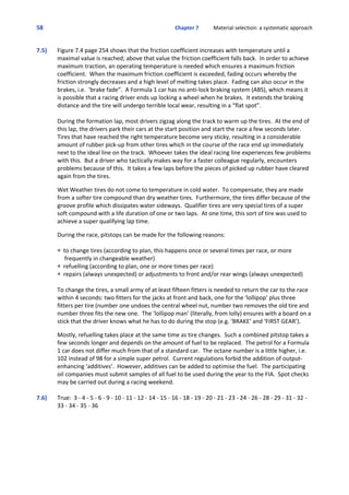
Problem 1.4: Driving torque tapered shaft hubs
The torque T that can be transmitted by a tapered shaft‐hub connection
is proportional to the clamping force, i.e. the bolt preload Fi. The preload
Fi is proportional to MA /μ where MA is the tightening torque μ the
coefficient of friction in the screw assembly. The coefficient of friction μ
is managed by using a proper thread lubricant and varies between 0.12
and 0.16. Calculate the coefficient of variation CV’=(T50 ‐Tmin) /T50 where
Tmin is the least torque that can be transmitted by the shaft‐hub
connection.](https://image.slidesharecdn.com/solutions-manual-dynamics-150924223223-lva1-app6891/85/Solutions-manual-dynamics-3-320.jpg)
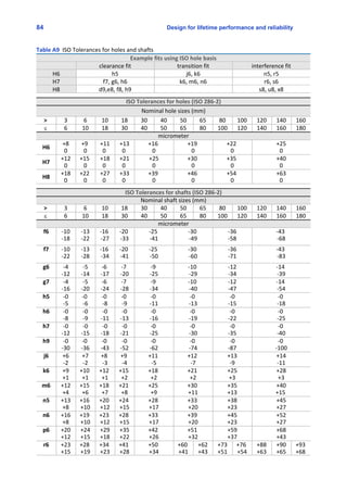
![Design for lifetime performance and reliability 7
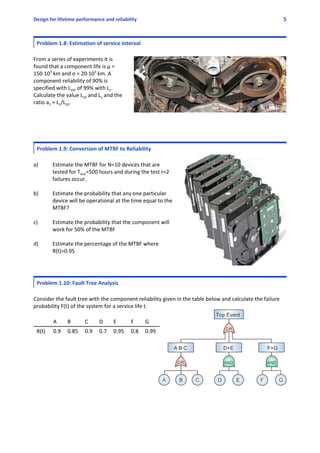
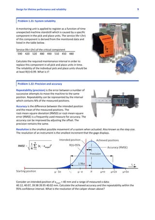
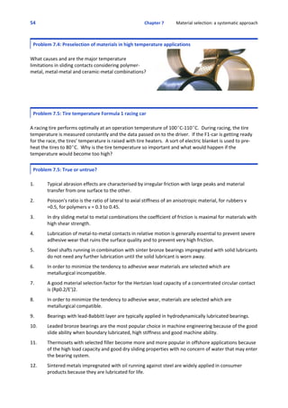
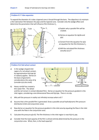
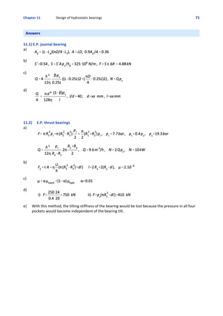
Problem 1.16: System reliability
Calculate the failure probability F(100 hr) of two
critical components of a system connected in series.
From product catalogues it is found that the reliability
of one component is specified with μ = 150 hr and σ =
30.5 hr, the other component is specified with μ = 120
hr and σ = 10.2 hr.
Hint: first step is to calculate R(t) of both components.
Problem 1.17: System reliability
A heavy‐duty motorized frame features a quad drive
system using two high power DC motors and four drive
belts. All four belts are required to maintain optimal
control. From field testing it is found that the service life
of the belts under heavy duty operating conditions is
normally distributed with a mean µ = 200 hr and a
standard deviation of σ = 0.2µ. Calculate the operating
reliability of the set of 4 belts for a service life of 150 hr.
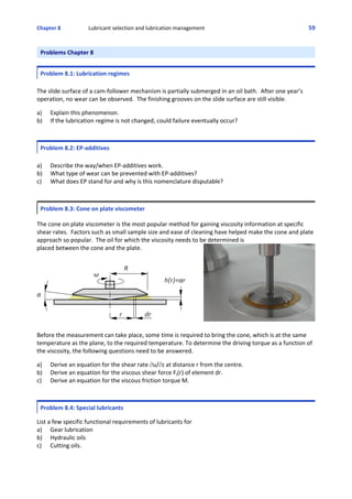
Problem 1.18: System reliability
There is a rule of thumb that says that the bearing load P related
to the dynamic load rating of the bearing C is:
Normal loaded bearings P=0.06
Heavily loaded bearings P=0.12C
Consider a motor drive equipped with two ball bearings. One of
the bearings is loaded with P=0.1C, where C is the dynamic load
rating of bearing type 16004, C=7.28 kN. The motor rotates with
n=1400 rpm during 8 hours a day, 5 days a week it is 1920
hr/year. Calculate the life expectancy [years] of this bearing with
1% failure probability.
Hint: First calculated L10 and L10h. The life expectancy Lna of ball bearings is related to the L10 basic rating
life according Lna =a1 L10 (Table 4.6 page 129).](https://image.slidesharecdn.com/solutions-manual-dynamics-150924223223-lva1-app6891/85/Solutions-manual-dynamics-7-320.jpg)
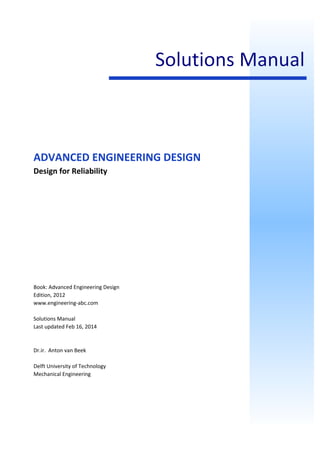
![12 Design for lifetime performance and reliability
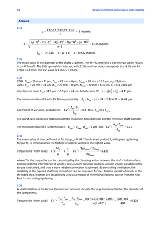
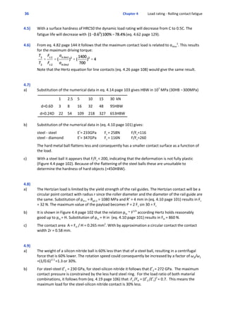
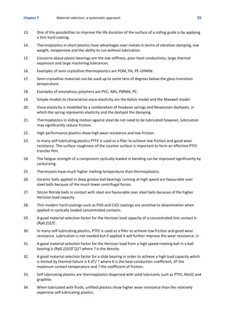
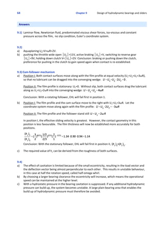
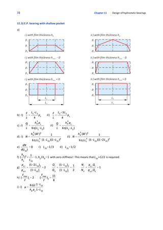
1.9)
The Mean Time Between Failure MTBF = T/r = TtestAn / r = 10A500/2 = 2500 hr / failure
The failure rate λ is the inverse of the MTBF, λ = 1/MTBF = 1 / 2500 = 0.04% / hr
The reliability R(t)=exp(‐λt) according (eq. 1.4 page 12), R(MTBF) = exp(‐1) = 0.37 = 37%
The probability that the component will work for 50% of the MTBF is R(t)=exp(‐0.5)=0.61
R(t)=0.95 is obtained with ‐ln(0.95)=0.0513 MTBF, only 5% of the MTBF.
1.10) F(t) = 1 ‐ AABAC A [ 1‐ (1‐D) (1‐E) ] [ 1‐ (1‐F) (1‐G) ] = 32%
1.11)
1.12)
1.13)
1.14)
1.15)
A chain with 100 components (links) connected in series and component reliability 0.99 results in a
system reliability of 0.99100
=0.366. If, one of the components has component reliability 0.95 (the
weakest link in the chain), the system reliability becomes 0.9999
@0.95=0.351. The conclusion is that “A
chain is only as strong as its weakest link” is valid in a deterministic approach, and it is the criterium for
failure by overload. In the case of a probabilistic approach which is necessary for reliability analysis if the
failure mode is fatigue, the reliability of all components matter.
1.16)
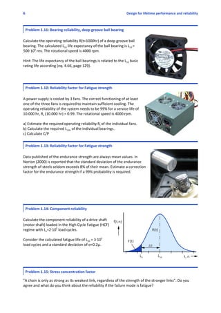
1.17)
Reliability factors Creliab for σ=0.08μ
R(t) 50% 90% 99% 99.9%
Creliab 1.000 0.897 0.814 0.753
Standard deviation σ = 0.08μ
Ln = μ‐zσ, 99% reliability, n=1, z=2.33
L50 = μ, 50% reliability
Creliab = Ln/L50, L1/L50=(μ ‐ zAσ)/μ = 0.814](https://image.slidesharecdn.com/solutions-manual-dynamics-150924223223-lva1-app6891/85/Solutions-manual-dynamics-12-320.jpg)
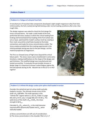
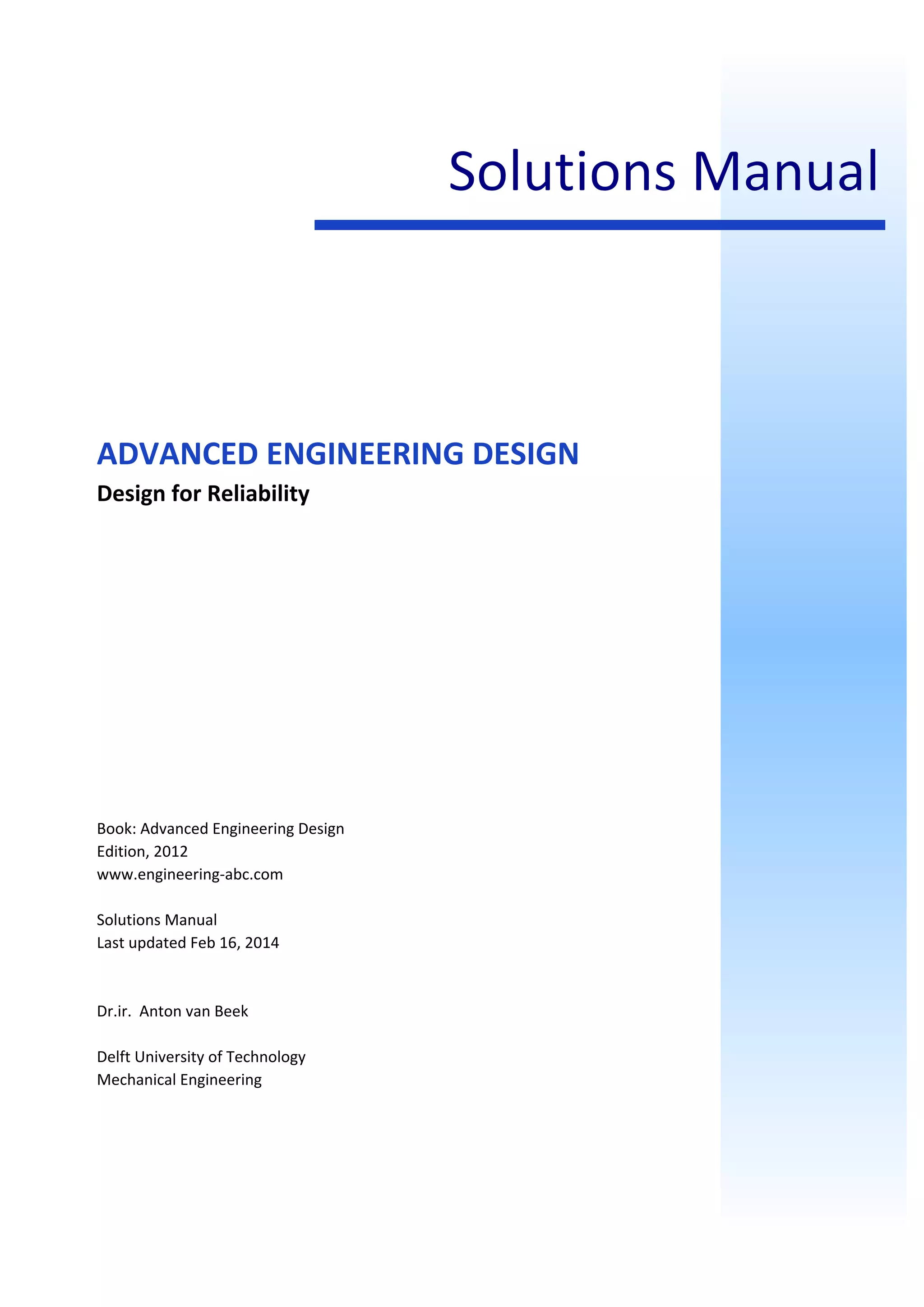
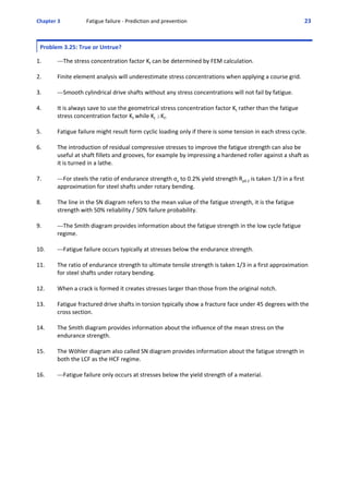
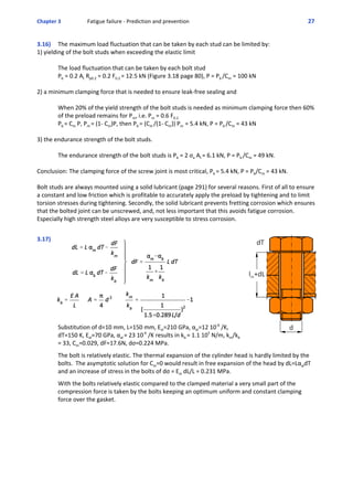
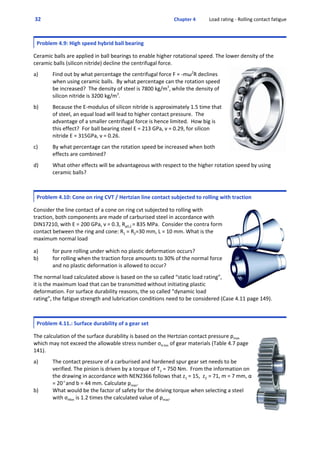
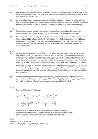
![Chapter 3 Fatigue failure ‐ Prediction and prevention 15
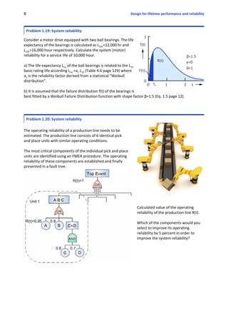
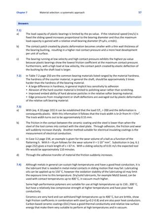
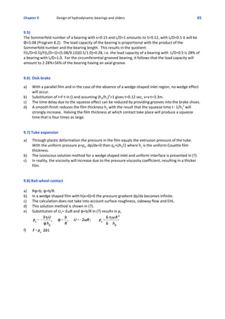
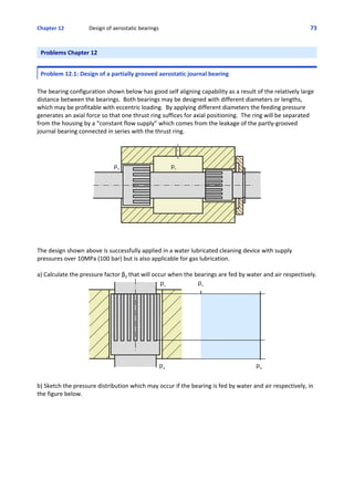
Problem 3.3: Infinite life design drive shaft with transverse hole loaded in torsion
Consider a drive shaft with transverse hole cyclically loaded in torsion with T = ±10 Nm. The ultimate
tensile stress of the shaft is Rm = 500 MPa, the yield stress of the shaft is Rp0.2 = 0.6Rm. The diameter of the
transverse hole in the shaft is related to the diameter of the shaft according d/D = 0.2. Calculate the
diameter of the shaft when:
a) statically loaded. Hint:
b) cyclically loaded in the “infinite life” regime where σ’e = 0.5Rm (Table 3.1 page 69), σe= 0.7σ’e and
τe=0.58σe. The stress concentration factor can be calculated with the curve fit function Kt=1.5899‐0.6355
log(d/D).
Problem 3.4: Infinite life design drive shaft under rotary bending
A stepped shaft is subjected to rotary bending M = 4 Nm. The ultimate tensile stress of the shaft is Rm =
500 MPa, the yield stress of the shaft is Rp0.2 = 0.6Rm. Calculate the
diameter of the shaft when:
a) statically loaded.
b) cyclically loaded in the “infinite life” regime where σ’e = 0.5Rm
(Table 3.1 page 69), σe = 0.7σ’e and Kt = 2.5.
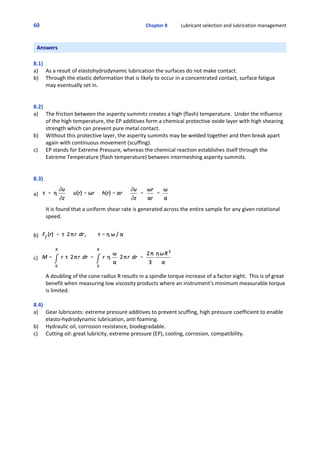
Problem 3.5: Infinite life design drive shaft under rotary bending
Calculate M1/M2 where
‐ M1 is the endurance strength for rotary bending of a 12 mm diameter shaft without groove and
‐ M2 is the endurance strength for rotary bending of a grooved shaft of d=20 mm, dk=19 mm and Kt=5.
Problem 3.6: Infinite life design drive shaft under rotary bending
Consider a grooved shaft in rotary bending. The diameter of the shaft d = d1 = 20 mm, the diameter of
the groove dk = 19 mm. The stress concentration factor Kt = 5. Calculate how much weight can be saved
when this shaft is replaced by an un‐grooved shaft of smaller diameter d2 with the same endurance
strength.
Calculate the percentage [%] of weight saving (m1‐m2)/m1 where m1
is the mass of the grooved shaft and m2 is the mass of the ungrooved
shaft.](https://image.slidesharecdn.com/solutions-manual-dynamics-150924223223-lva1-app6891/85/Solutions-manual-dynamics-15-320.jpg)
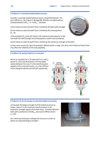
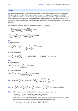
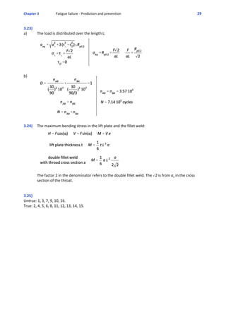
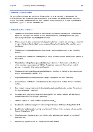
![18 Chapter 3 Fatigue failure ‐ Prediction and prevention
Problem 3.13: Improved fatigue strength piston ‐ rod connection
Consider two possible configurations for a hydraulic piston ‐ rod connection.
Configuration 1) M24‐8.8, clamped over Lm=d, preloaded with 0.8F0.2
Configuration 2) M12‐8.8, clamped over Lm=3d, preloaded with 0.8F0.2
Calculate the ratio of the
fatigue strength P2/P1. P1 and
P2 are the piston forces of
configuration 1 and 2
respectively, that can be
sustained for infinite life. The
small letter p is the hydraulic
pressure.
Problem 3.14: Fatigue failure probability of a screw joint
Consider a pneumatic cylinder that consists of an aluminium bushing
with two end caps clamped by 4 steel bolt studs.
Bolt studs: db=4 mm, Esteel=210 GPa
Bushing: Dcyl=80mm, wall thickness s=6 mm, Ealum=70 GPa
a) Calculate the joint stiffness factor Cm.
b) The bushing is replaced by one with a 3 mm wall thickness. So, the
joint stiffness factor of a screw joint is not Cm=1/4.2 but becomes
Cm=1/2.6. What consequences will this deviation in joint stiffness
have for the fatigue strength of the bolted connection.
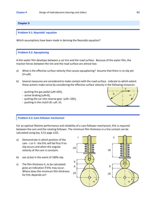
Problem 3.15: Improved fatigue strength using stretch bolts
Stretch bolts are used by car manufacturers for several reasons; to
accommodate LCF thermal expansion (thermo‐mechanical fatigue
TMF), to withstand HCF load and finally they can be prestressed
accurately.
a) Calculate the stress concentration factor in the threaded section of
the bolt. Consider a metric M12‐8.8 bolt and an endurance strength of
the steel when loaded in axial tension of σ’e =0.4Rm. The fatigue
strength of the threaded part σa=50 MPa is derived from Figure 3.16 page 79.
b) Calculate the minimal diameter of the shank, if the same fatigue strength [N] is asked for the shank
and the threaded section. The stress concentration in the fillet on both ends of the shank is Kt=1.8. The
strength reduction factors in the shank are C surf C reliab = 0.8.](https://image.slidesharecdn.com/solutions-manual-dynamics-150924223223-lva1-app6891/85/Solutions-manual-dynamics-18-320.jpg)

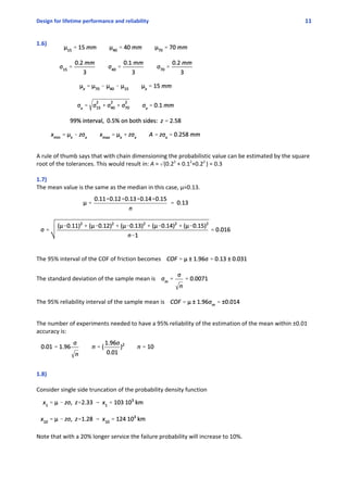
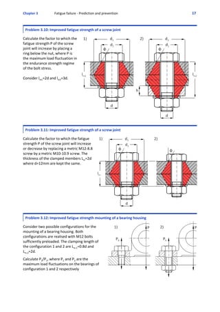
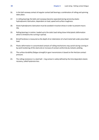
![20 Chapter 3 Fatigue failure ‐ Prediction and prevention
Problem 3.19: Infinite life design compression spring
Calculate the max amplitude of a compression spring for infinite
life. Consider a wire diameter d=10 mm, number of winds n=8,
radius of the winds r=50 mm, a shear modulus of G=80 GPa, Rm =
2220 ‐ 820 log d where d [mm] and Rm [MPa], a fatigue strength for
107
stress cycles of τe /Rm=0.15. Approximate equations for spring
stiffness of coil springs are listed in Table A4 page 526.
Problem 3.20: Finite life design of a welded chassis
Two hot rolled steel sections of S235
(Rp0.2 =235 MPa) are connected by
welding. The fatigue strength of the
welded zone is characterised σHCF
(N=107
) = 30 MPa (SN‐diagram shown
below).
Calculate the number of stress cycles
that can be sustained with stresses as
high as the yield strength of the
structural steel itself.
Problem 3.21: Finite life design of butt‐weld connections in pipe flanges
Socket weld pipe flanges actually slip over the pipe. These pipe flanges
are typically machined with an inside diameter slightly larger than the
outside diameter of the pipe. Socket pipe flanges, are secured to the
pipe with a fillet weld around the top of the flange.
Weld neck flanges attach to the pipe
by welding the pipe to the neck of
the pipe flange with u butt weld.
The neck allows for the transfer of
stress from the weld neck pipe flanges to the pipe itself. Weld neck
pipe flanges are often used for high pressure applications. The inside
diameter of a weld neck pipe flange is machined to match the inside
diameter of the pipe.](https://image.slidesharecdn.com/solutions-manual-dynamics-150924223223-lva1-app6891/85/Solutions-manual-dynamics-20-320.jpg)
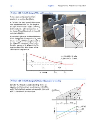
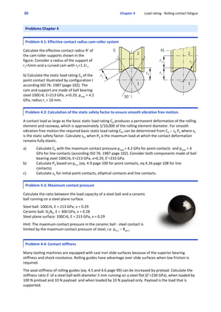
![Chapter 3 Fatigue failure ‐ Prediction and prevention 21
Calculate the ratio of the fatigue life of the weld connection in a “socket weld pipe flange” with respect
to the “weld neck pipe flange”, Ns/Nn. The Socket weld flange is typically a detail category with
σHCF(N=107
)=30 MPa, the weld neck flange with σHCF(N=107
)=45 MPa (SN‐diagram shown in previous
problem). Consider a fatigue load inducing a stress over the cross section of the pipe of 50 MPa.
Problem 3.22: Finite life design of butt‐weld connections using the Palmgren‐Miner rule
Steel grades known as S235, S275 and S355 are non‐alloy structural steels. The steel grades of the JR, JO,
J2 and K2 categories are in general suitable for all welding techniques. The yield strength of S235 for
example is 235 MPa. The strength of butt welds when statically loaded do not need to be calculated
separately, since the strength of the weld material is at least as strong as that of the structural steel.
A reasonable estimation of the endurance strength of structural steels made of S235 subjected to cyclic
bending is σe = 0.4Rm . 160 MPa, which is 70% of the yield strength .
The endurance strength of welded connections is much less than the endurance strength of the
structural steel members. For example, the endurance strength of butt welds is limited to approximately
σe=0.55A45.25 MPa (Figure 3.30 page 90 and Figure 3.27 page 87), which is less than 20% of the
endurance strength of the structural steel S235.
σHCF (N=107
) = 45 MPa
σe (N=2A108
) = 25 MPa
The relatively low value of the endurance strength of welded connections and the relative high stress
peaks that must be sustained during life makes that most welded structures are designed in the “finite
life regime”. Since parts are seldom stressed repeatedly at only one stress level, the cumulative damage
effect of operations at various levels of stress need to be considered.
Calculate the fatigue life L(hr) of a welded connection located between the cylinder bushing and the end
cap of a hydraulic cylinder.
The actual stresses in the weld are measured
during one hour of service. The stress
spectrum is simplified into the values which
are listed in the table below.
σF [MPa] 240 120 60 30 20
ni [‐] 10 20 40 400 1000](https://image.slidesharecdn.com/solutions-manual-dynamics-150924223223-lva1-app6891/85/Solutions-manual-dynamics-21-320.jpg)
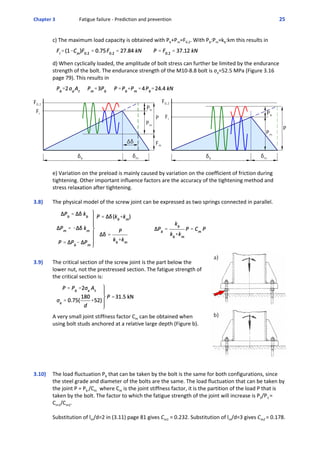
![28 Chapter 3 Fatigue failure ‐ Prediction and prevention
3.18)
This model can be useful to analyse the possibility of corrective actions.
3.19)
3.20) Substitution of σHCF=30 MPa, σi=235 MPa, m=3 in
3.21) The fatigue life expressed in the number of stress cycles Ni is calculated with eq. 3.12 page 87.
Ns/Nn=(30/45)3
=0.296. The exponent m=3 for both flanges since σi > σHCF. Note that the fatigue
life of the socked flange is only 30% of the fatigue life of the neck flange.
3.22) First step is to calculate the damage fraction D for one hour of service.
The damage fraction D=ni/Ni where Ni is the number of load cycles that could be accumulated
when the amplitude of the stress cycles would remain constant over life (eq 3.12 page 87).
Δσi [MPa] 240 120 60 30 20
ni [‐] 10 20 40 400 1000
Ni [‐]
Hypothetical: If in one hour D = ni/Ni = 0.1, then 10% of the service life has passed and the service
life would be L = 1/D = 10 hours.
The fatigue life is achieved when the cumulative damage D=1. So, the service life L becomes:](https://image.slidesharecdn.com/solutions-manual-dynamics-150924223223-lva1-app6891/85/Solutions-manual-dynamics-28-320.jpg)

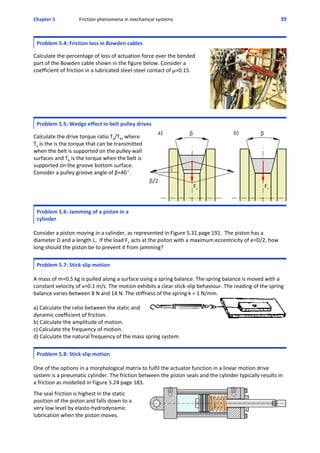
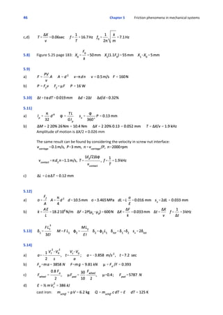
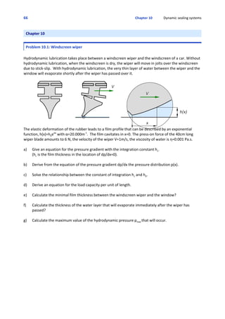
![40 Chapter 5 Friction phenomena in mechanical systems
Consider a pneumatic cylinder ‐ spring system. The static friction between the piston and cylinder wall
can be expressed as a percentage of the piston force Fstat = 10% Fpiston. The piston is actuated by air
pressure. The air pressure is increased until the piston starts to move. When the piston starts to move
the friction falls down to approximate zero level. The piston will make a step forward. This process is
repeated.
Calculate the smallest possible step size in a step by step movement of the piston. Start from a position
in which there is equilibrium between the air pressure and the spring force (zero friction). In this position
F0 = 500 N. Next the air pressure is increased until the piston starts to move etc. The spring stiffness k=10
N/mm.
Problem 5.9: PV‐value
Consider a polymer bearing with a PV‐value of PV = 0.2 MPa Am/s. The shaft
diameter d=20 mm, the bearing width L=d, rotational speed n=477 rpm.
a) Calculate the load that this bearing can sustain.
b) Calculate power loss in this bearing at the moment of failure, assuming a
coefficient of friction μ=0.2
Problem 5.10: Operating clearance
If a bearing bushing is press fitted in a metal housing a cumulation of machining tolerances result in a
large variation of the bearing busing inside diameter. To ensure a positive clearance under the most
unfavourable conditions the minimum value of the operating clearance in generally is taken to be 0.5% of
the shaft diameter. The operating clearance is defined as the minimum clearance during operation.
Effects resulting in a decrease of clearance during operation are thermal dimensional changes and for
some polymers moisture‐related dimensional changes.
Calculate the decrease of the bearing clearance [%] of a PA plain bearing bushing with a shaft diameter of
d=12 mm and a wall thickness of t=3 mm. Consider a temperature increase of the polymer of dT=80
degrees and a linear expansion coefficient of PA of α=80 10‐6
/K
Problem 5.11: Hysteresis error from friction in the drive spindle
In the figure below a linear motion axis of a milling machine is shown actuated by a servo motor. The
system accuracy suffers from the “Wind‐up” of the lead screw. The “Wind‐up” of drive shafts is defined
as the torsion angle. It is assumed that the displacement of the carriage is set by the rotation angle of a
stepper motor. The drive torque is present in one direction of motion.
Screw length L = 1 m
Trapezoidal thread Tr12 x P3
Pitch diameter d2 = 10.5 mm
Shear modulus G = 80 GPa
Drive torque Tdyn = 26 Nm
Drive torque Tstat = 1.2 Tdyn
v = 0.1 m/s
a) Calculate the hysteresis error resulting from the friction in the drive spindle.](https://image.slidesharecdn.com/solutions-manual-dynamics-150924223223-lva1-app6891/85/Solutions-manual-dynamics-40-320.jpg)
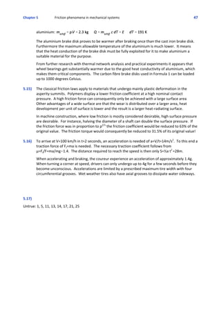
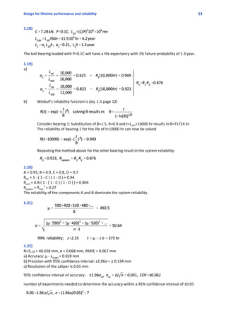
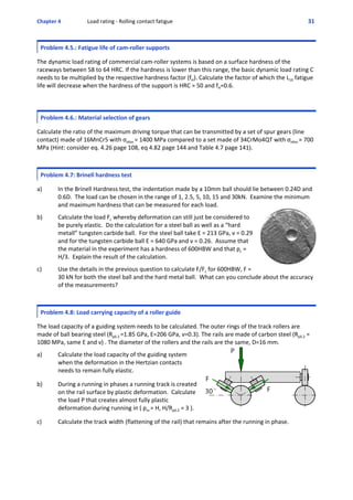
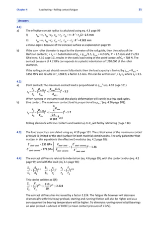
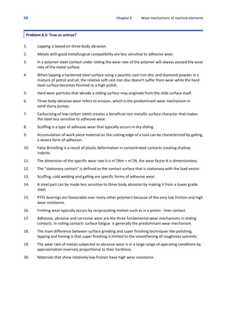
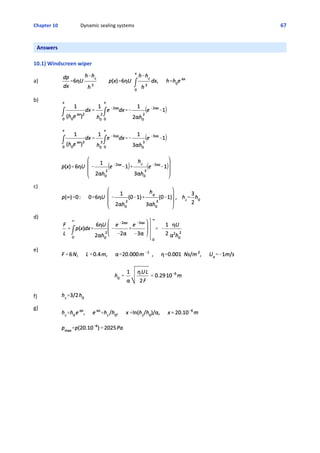
![48 Chapter 6 Wear mechanisms of machine elements
Problems Chapter 6
Problem 6.1: Service life of a lead screw
Consider a lead screw assembly that operates with a contact pressure in the threaded area of p = 5 MPa.
The pitch diameter d2=10.5 mm. The stroke over which the nut is displaced is 20 times the nut height.
The number of loaded turns during service life is n=100 103
rev.
The specific wear rate of the bronze
nut and the spindle are knut = kspindle =
10 10‐15
m2
/N. Calculate the increase of
backlash h [mm] in the screw‐nut
interface of a trapezoidal lead screw
a) caused by wear of the bronze nut.
b) caused by wear of the spindle.
Problem 6.2: Investigation to hard wearing materials for knee replacements
In order to assess the wear performance of different materials of total knee replacements (TKR), a block
on ring test rig will be used. The ring is actuated in reciprocating motion.
a) Calculate the required test duration in hours.
The ring is made of steel, the block from ultra high weight molecular polyethylene (UHMWPE). The
density of UHMWPE is ρ = 945 kg/m3
. A specific wear rate k=10∙10‐15
m2
/N of the PE block is expected. A
minimum wear of the polymer block of 0.1 gram is to be obtained to establish the wear rate. The contact
surface A=100 mm2
, the surface pressure is p=2 MPa, the total sliding distance in one cycle is si = 30 mm
and n=2 cycles per second are made.
b) What temperature will the ring get when the frictional heating is to be transferred by convection only.
The coefficient of friction μ=0.12, the heat convection coefficient of the rotating disc in free air hc = 80
W/ m2
K and the effective heat convection surface area of the ring A = 7 10‐3
m2
.](https://image.slidesharecdn.com/solutions-manual-dynamics-150924223223-lva1-app6891/85/Solutions-manual-dynamics-48-320.jpg)
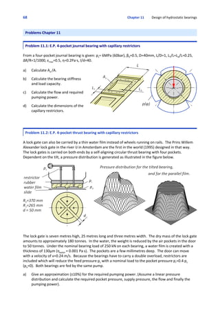
![Chapter 6 Wear mechanisms of machine elements 49
Problem 6.3: Service life of a linear axis using plain bearings
A linear guide’s travel smoothness and tolerance variations are key concerns for machine designers. But,
the most important design factor is how well the guide resists deflection. Linear support rails in
combination with open design bearings are best suited to sustain heavy loads and to provide high
stiffness.
Linear plain bearings are the better choice
compared to linear ball bearings when the bearing
arrangement is subjected to heavy shock loads,
vibrations or high accelerations in the unloaded
state however, increased friction must be expected.
Calculate over what sliding distance s [km] the
bearing will wear down over h=0.1 mm. Consider a
mean value of the contact pressure of p = 3 MPa
and the specific wear rate of k= 10‐15
m2
/N.
Consider good conformity between the plain
bearing and the linear support.
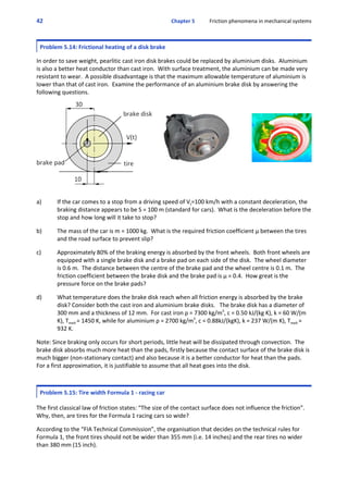
Problem 6.4: Service life disk brake
a) Calculate the service life of disk brake pads, expressed
in numbers of brake times. The contact area of the
brake pad is approached by a round disk with a
diameter of d=60mm located at centre distance
r=100mm, the thickness of the brake lining is
t=10mm, the specific wear rate k=50 10‐15
m2
/N (class
5), the normal force F=6000N, the wheel diameter
D=0.6m and the brake distance S=100 m.
b) How much thinner will the brake disk worn down
during the service life of the brake pads if the specific
wear rate of the brake disk equals that of the brake
lining?
c) What is the perfect ratio of kpad/kdisk that makes that
the pad and disk are worn after the same sliding
distance if hpad/hdisk = 5?](https://image.slidesharecdn.com/solutions-manual-dynamics-150924223223-lva1-app6891/85/Solutions-manual-dynamics-49-320.jpg)


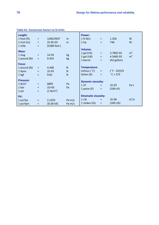
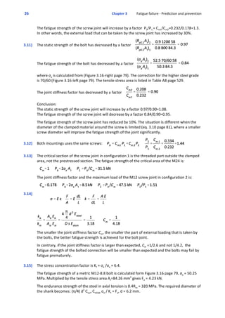
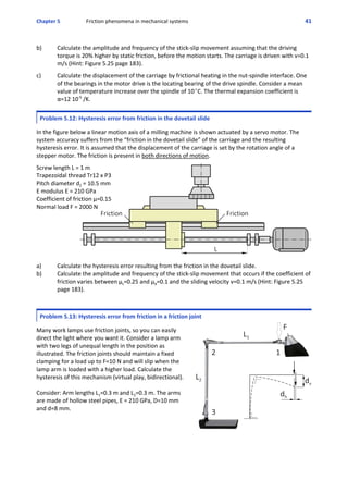
![Design for lifetime performance and reliability 81
Table A5 Buckling limit of compression loaded beams [Gero & Timoshenko, 1985]
Table A6 Approximate design functions S‐shaped beams [Koster, 1996]
leaf spring wire spring leave spring wire spring
longitudinal
stiffness
cxx
lateral
stiffness
czz
bending
stress
σψz
buckling load
Fk
1)
The configuration with reinforced mid‐section considered in this table shows an increase of the
buckling load by a factor of nine while the lateral stiffness has increased with only 20%.](https://image.slidesharecdn.com/solutions-manual-dynamics-150924223223-lva1-app6891/85/Solutions-manual-dynamics-81-320.jpg)
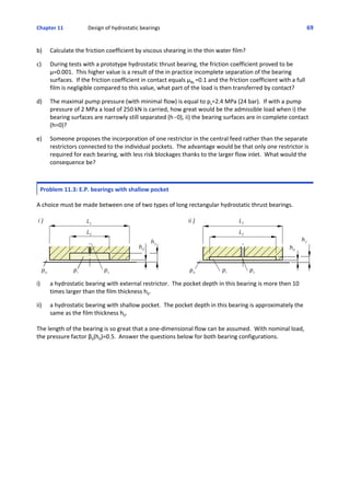
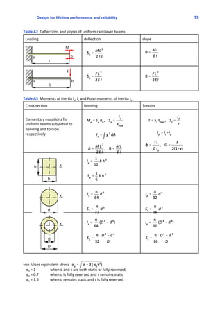
![82 Design for lifetime performance and reliability
21
2
I mr
Table A7 Moments of Inertia
Moment of inertia: Radius of gyration :
2
I dm i I m
Parallel axis theorem : Torque :
2
zI I a m T I
Linear motion Rotational motion
Position x Angular position n
Velocity v Angular velocity ω
Acceleration a Angular acceleration α
Load F [ N ] moment M [ Nm ]
mass m [ kg ] moment of inertia I [ kg m2
]
Impulse p = m v [kg m/s] Angular Momentum H = I ω [kg m2
/s]
F = m a [N = kg m/s2
] M = I α [ Nm = kg m2
rad/s2
]
W = F s [ N m = J ] W = M n [ Nm rad = J ]
Ek = ½ mv2
[ J ] Ek = ½ I ω2
[ J ]
P = W/t = F s / t [ J/s = W ] P = W/t = M ω [ J/s = W ]
22
5
I mr](https://image.slidesharecdn.com/solutions-manual-dynamics-150924223223-lva1-app6891/85/Solutions-manual-dynamics-82-320.jpg)