D
r
a
f
t
The Project PlanningProcess
• Objective: provides a framework that enables the project
manager to make reasonable estimates of resources, cost, and
schedule.
• Estimates define best-case and worst-case scenarios so that
project outcomes can be bounded.
2.
D
r
a
f
t
Task Set forProject Planning
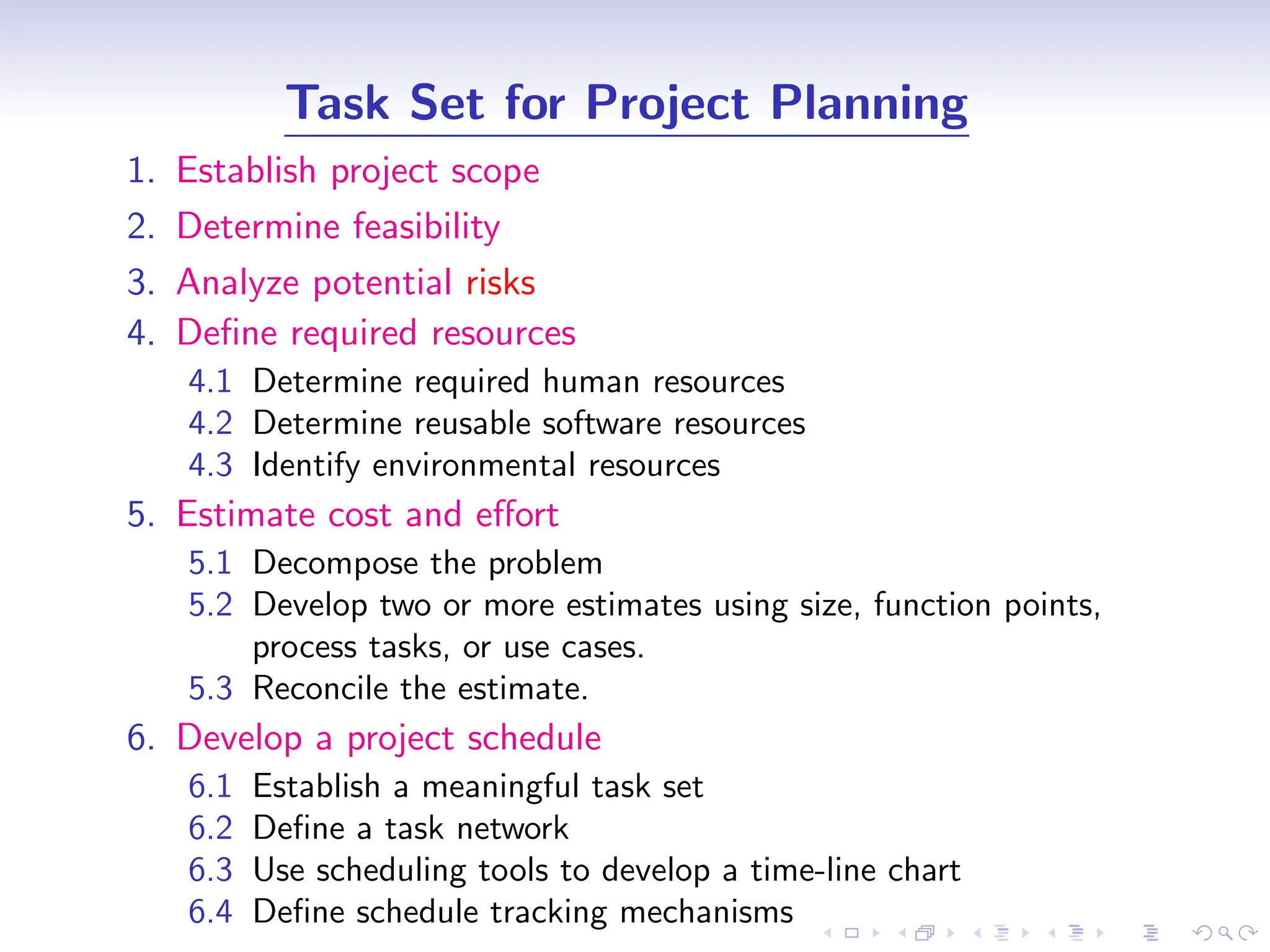
1. Establish project scope
2. Determine feasibility
3. Analyze potential risks
4. Define required resources
4.1 Determine required human resources
4.2 Determine reusable software resources
4.3 Identify environmental resources
5. Estimate cost and effort
5.1 Decompose the problem
5.2 Develop two or more estimates using size, function points,
process tasks, or use cases.
5.3 Reconcile the estimate.
6. Develop a project schedule
6.1 Establish a meaningful task set
6.2 Define a task network
6.3 Use scheduling tools to develop a time-line chart
6.4 Define schedule tracking mechanisms
3.
D
r
a
f
t
Software Scope andFeasibility
Software Scope: describes
• the functions and features that are to be delivered to end
users;
• the data that are input and output;
• the content that is presented to users as a consequence of
using the software; and
• the performance (processing and response time consideration),
constraints (limits placed on the software by external
hardware, available memory, or other existing systems),
interfaces, and reliability that bound the system.
4.
D
r
a
f
t
Software Scope andFeasibility (cont.)
Software Scope is defined using one of the two techniques:
1. A narrative description of software scope is developed after
communication with all stakeholders.
2. A set of use cases is developed by end users.
5.
D
r
a
f
t
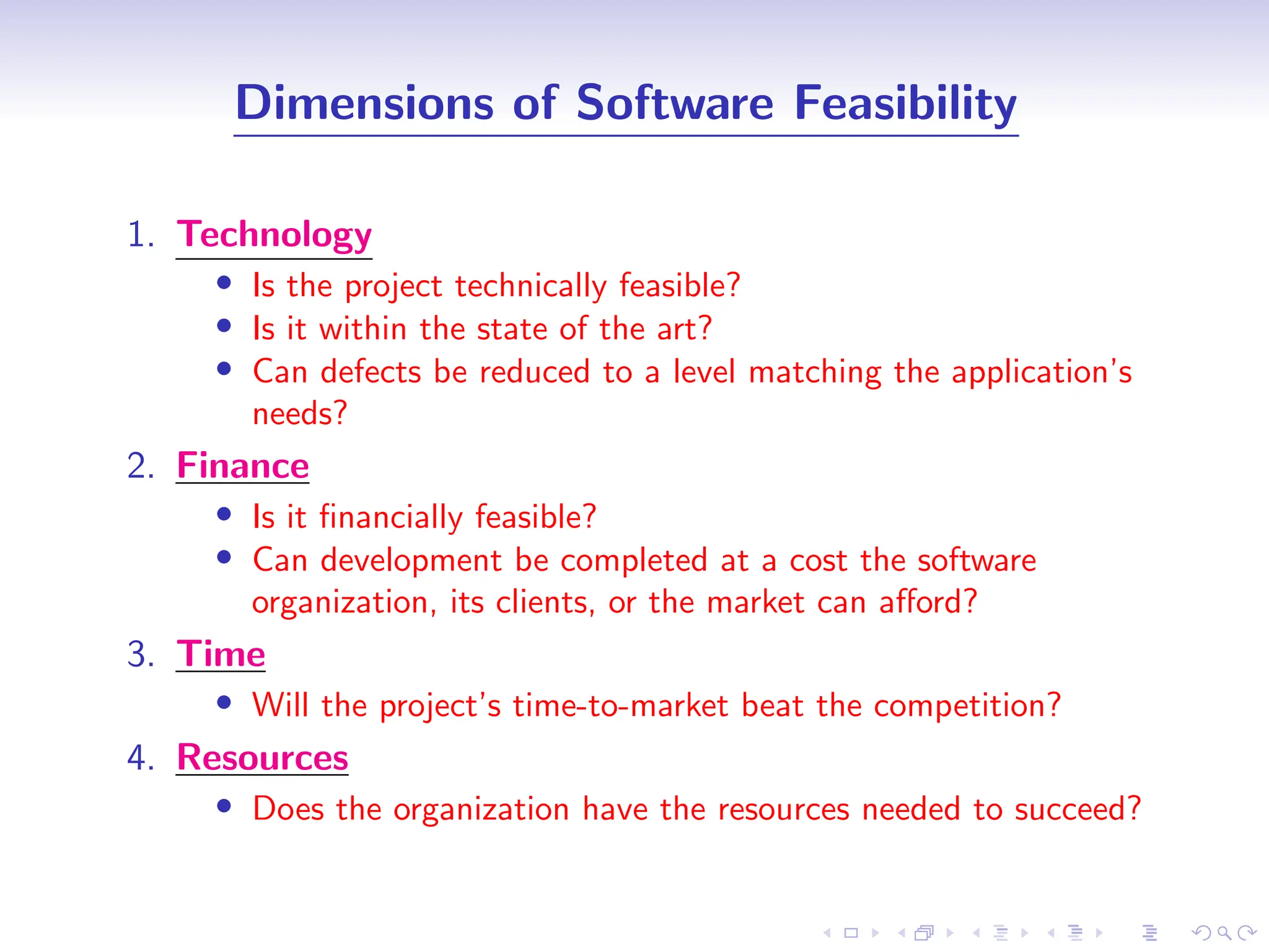
Dimensions of SoftwareFeasibility
1. Technology
• Is the project technically feasible?
• Is it within the state of the art?
• Can defects be reduced to a level matching the application’s
needs?
2. Finance
• Is it financially feasible?
• Can development be completed at a cost the software
organization, its clients, or the market can afford?
3. Time
• Will the project’s time-to-market beat the competition?
4. Resources
• Does the organization have the resources needed to succeed?
6.
D
r
a
f
t
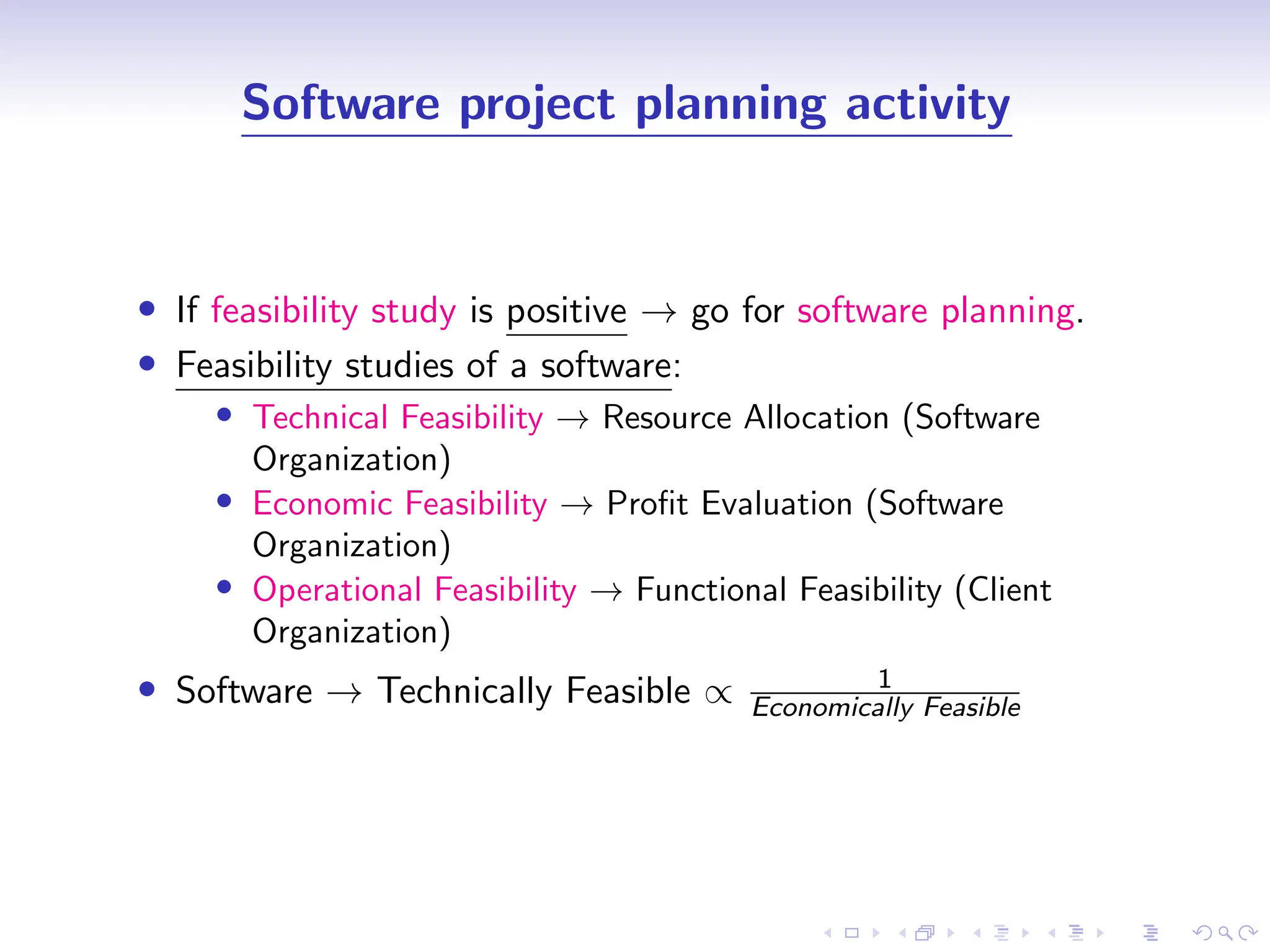
Software project planningactivity
• If feasibility study is positive → go for software planning.
• Feasibility studies of a software:
• Technical Feasibility → Resource Allocation (Software
Organization)
• Economic Feasibility → Profit Evaluation (Software
Organization)
• Operational Feasibility → Functional Feasibility (Client
Organization)
• Software → Technically Feasible ∝ 1
Economically Feasible
7.
D
r
a
f
t
Software project planningactivity (cont.)
• Software Project planning consists of following five major
activities:
• Estimation
• Scheduling
• Risk Analysis
• Quality management planning
• Change management planning
• Essence of Software Planning Activities
• Resource Estimation
• Effort Estimation
• Cost Estimation
• Time Estimation
8.
D
r
a
f
t
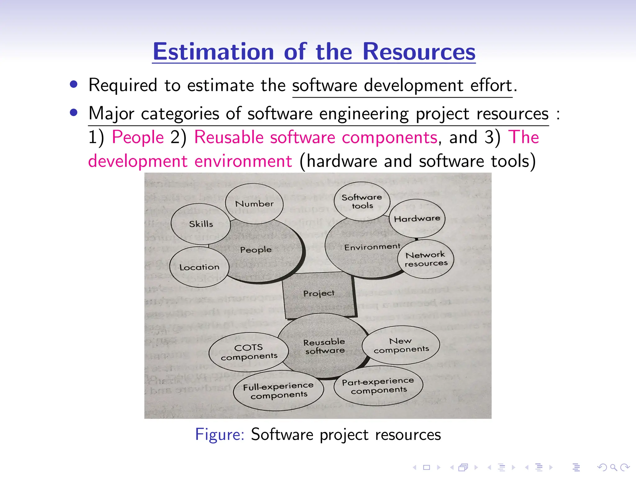
Estimation of theResources
• Required to estimate the software development effort.
• Major categories of software engineering project resources :
1) People 2) Reusable software components, and 3) The
development environment (hardware and software tools)
Figure: Software project resources
9.
D
r
a
f
t
Estimation of theResources (cont.)
1. Human Resource
• Focuses on the human skills required to complete the software
development.
• The number of people required for a software project can be
determined only after an estimate of development effort (e.g.,
person-months) is made.
10.
D
r
a
f
t
Estimation of theResources (cont.)
2. Reusable software resources
• Focus is on the creation and reuse of software building blocks
(components).
• Such components must be cataloged for easy reference,
standardized for easy application, and validated for easy
integration.
2.1 Off-the-shelf components
• Existing software that can be acquired from a third party or
from a past project.
• COTS (commercial off-the-shelf) components are purchased
from a third party, are ready for use on the current project,
and have been fully validated.
11.
D
r
a
f
t
Estimation of theResources (cont.)
2.2 Full-experience components
• Existing specifications, designs, code, or test data developed
for past projects that are similar to the software to built for
the current project.
• Members of the current software team have had full experience
in the application area represented by these components.
→ Therefore, modifications required for full-experience
components will be relatively low risk.
2.3 Partial-experience components
• Similar to fully-experience components but will require
substantial modification.
• Members of the current software team have only limited
experience in the application area represented by these
components.
→ Therefore, modifications required for partial-experience
components have a fair degree of risk.
2.4 New components
• Must be built by the software team specifically for the needs
of the current project.
12.
D
r
a
f
t
Estimation of theResources (cont.)
3. Environmental software resources
• Software engineering environment (SEE): the environment that
supports a software project (incorporates hardware and
software).
• Hardware: provides a platform that supports the tools (i.e.,
softwares) required to produce the work products (outcome of
good software engineering practice).
• When a computer-based system (incorporating specialized
hardware and software) is to be engineered, the software team
may require access to hardware elements being developed by
other engineering teams.
13.
D
r
a
f
t
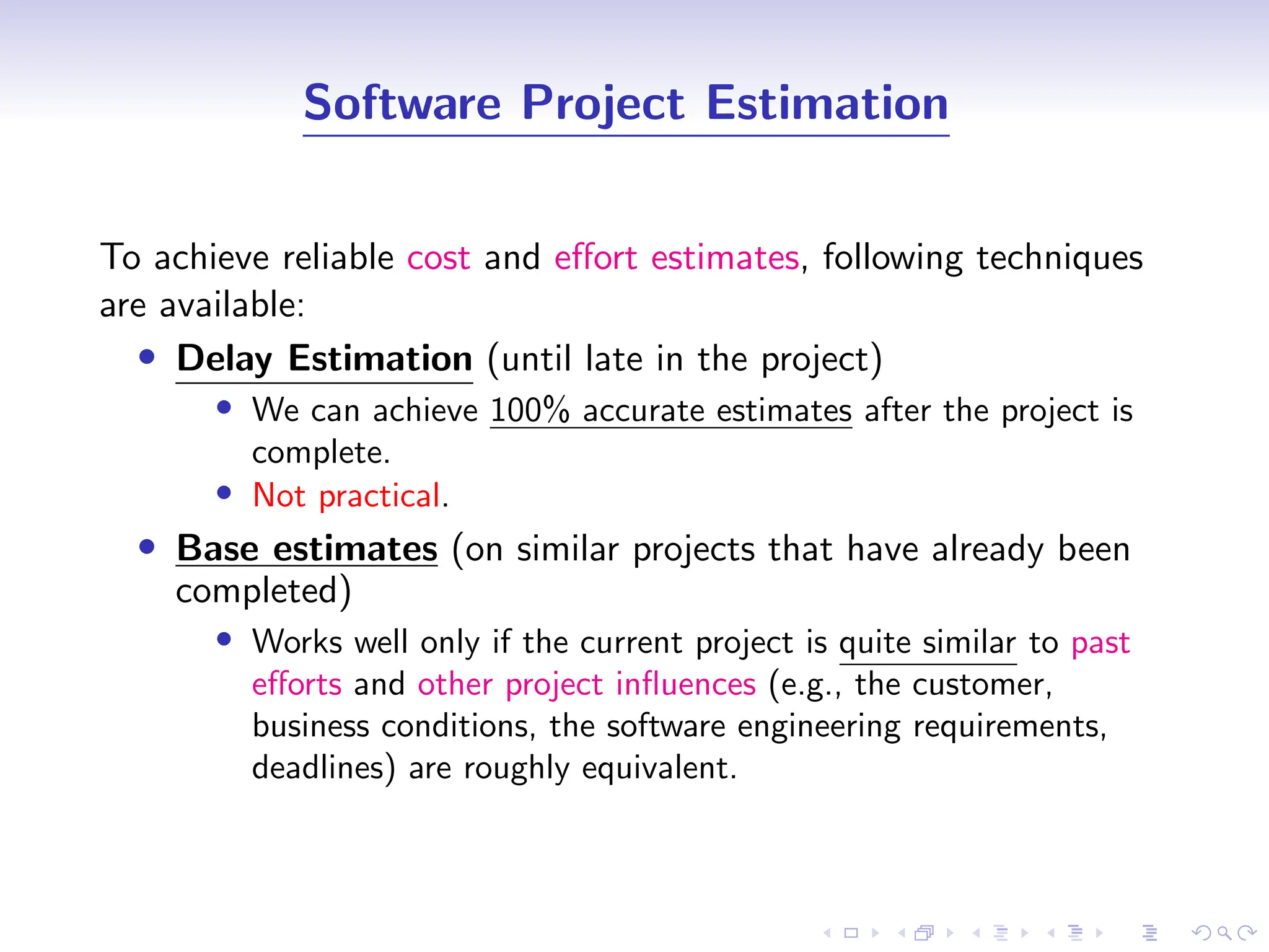
Software Project Estimation
Toachieve reliable cost and effort estimates, following techniques
are available:
• Delay Estimation (until late in the project)
• We can achieve 100% accurate estimates after the project is
complete.
• Not practical.
• Base estimates (on similar projects that have already been
completed)
• Works well only if the current project is quite similar to past
efforts and other project influences (e.g., the customer,
business conditions, the software engineering requirements,
deadlines) are roughly equivalent.
14.
D
r
a
f
t
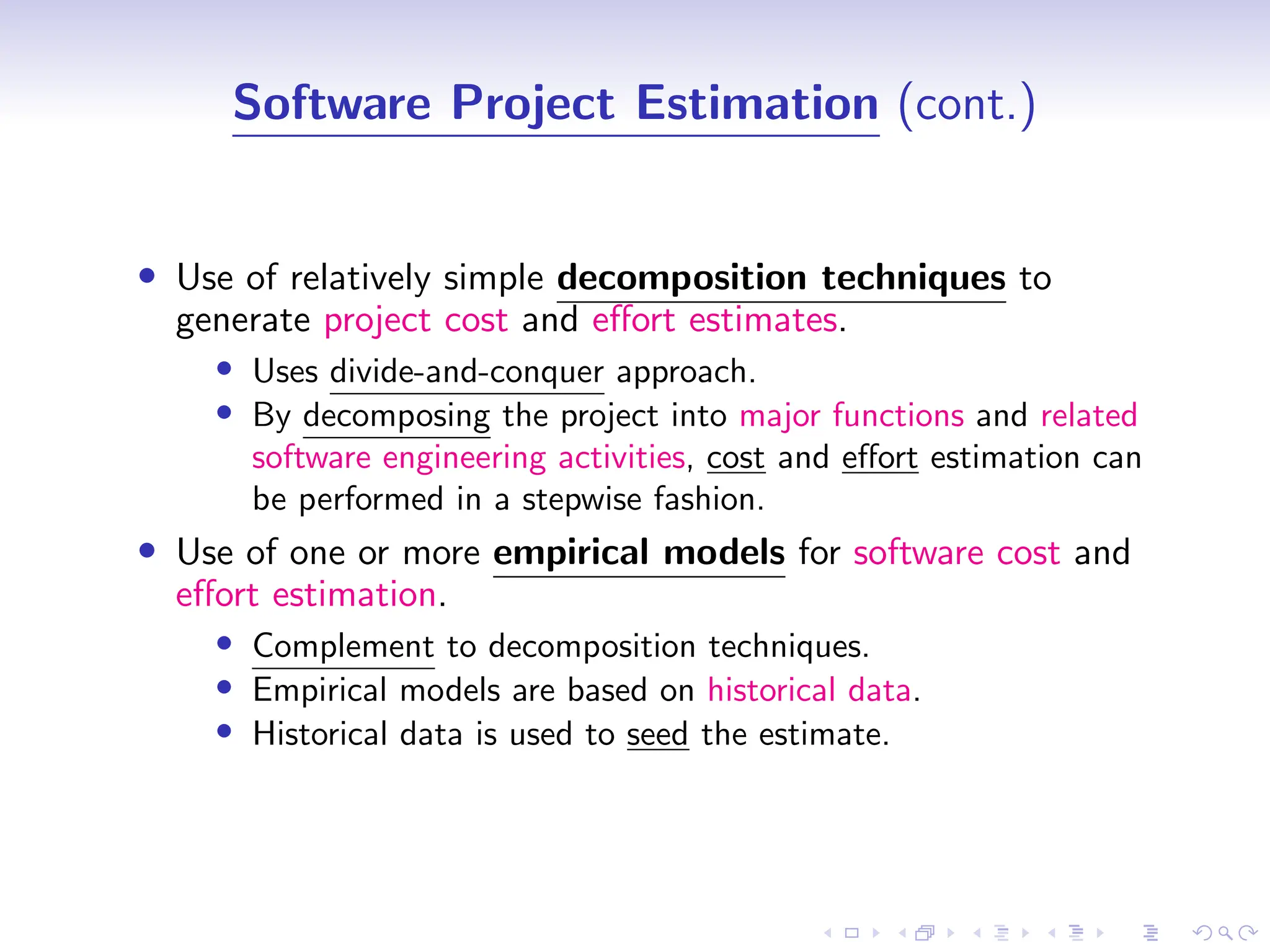
Software Project Estimation(cont.)
• Use of relatively simple decomposition techniques to
generate project cost and effort estimates.
• Uses divide-and-conquer approach.
• By decomposing the project into major functions and related
software engineering activities, cost and effort estimation can
be performed in a stepwise fashion.
• Use of one or more empirical models for software cost and
effort estimation.
• Complement to decomposition techniques.
• Empirical models are based on historical data.
• Historical data is used to seed the estimate.
15.
D
r
a
f
t
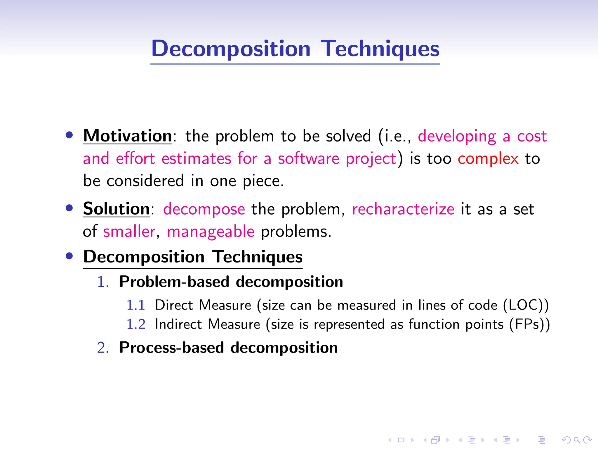
Decomposition Techniques
• Motivation:the problem to be solved (i.e., developing a cost
and effort estimates for a software project) is too complex to
be considered in one piece.
• Solution: decompose the problem, recharacterize it as a set
of smaller, manageable problems.
• Decomposition Techniques
1. Problem-based decomposition
1.1 Direct Measure (size can be measured in lines of code (LOC))
1.2 Indirect Measure (size is represented as function points (FPs))
2. Process-based decomposition
16.
D
r
a
f
t
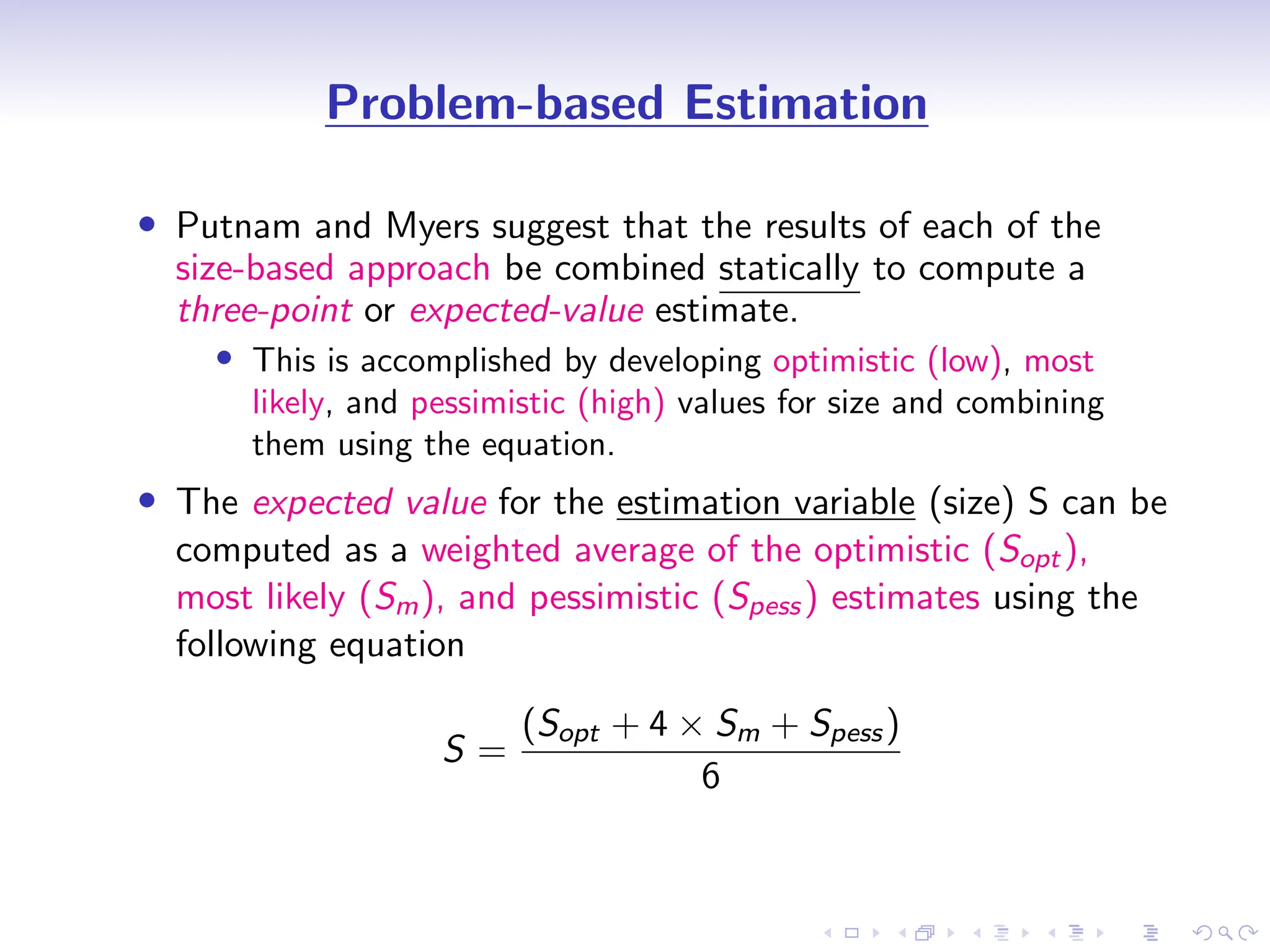
Problem-based Estimation
• Putnamand Myers suggest that the results of each of the
size-based approach be combined statically to compute a
three-point or expected-value estimate.
• This is accomplished by developing optimistic (low), most
likely, and pessimistic (high) values for size and combining
them using the equation.
• The expected value for the estimation variable (size) S can be
computed as a weighted average of the optimistic (Sopt),
most likely (Sm), and pessimistic (Spess) estimates using the
following equation
S =
(Sopt + 4 × Sm + Spess)
6
17.
D
r
a
f
t
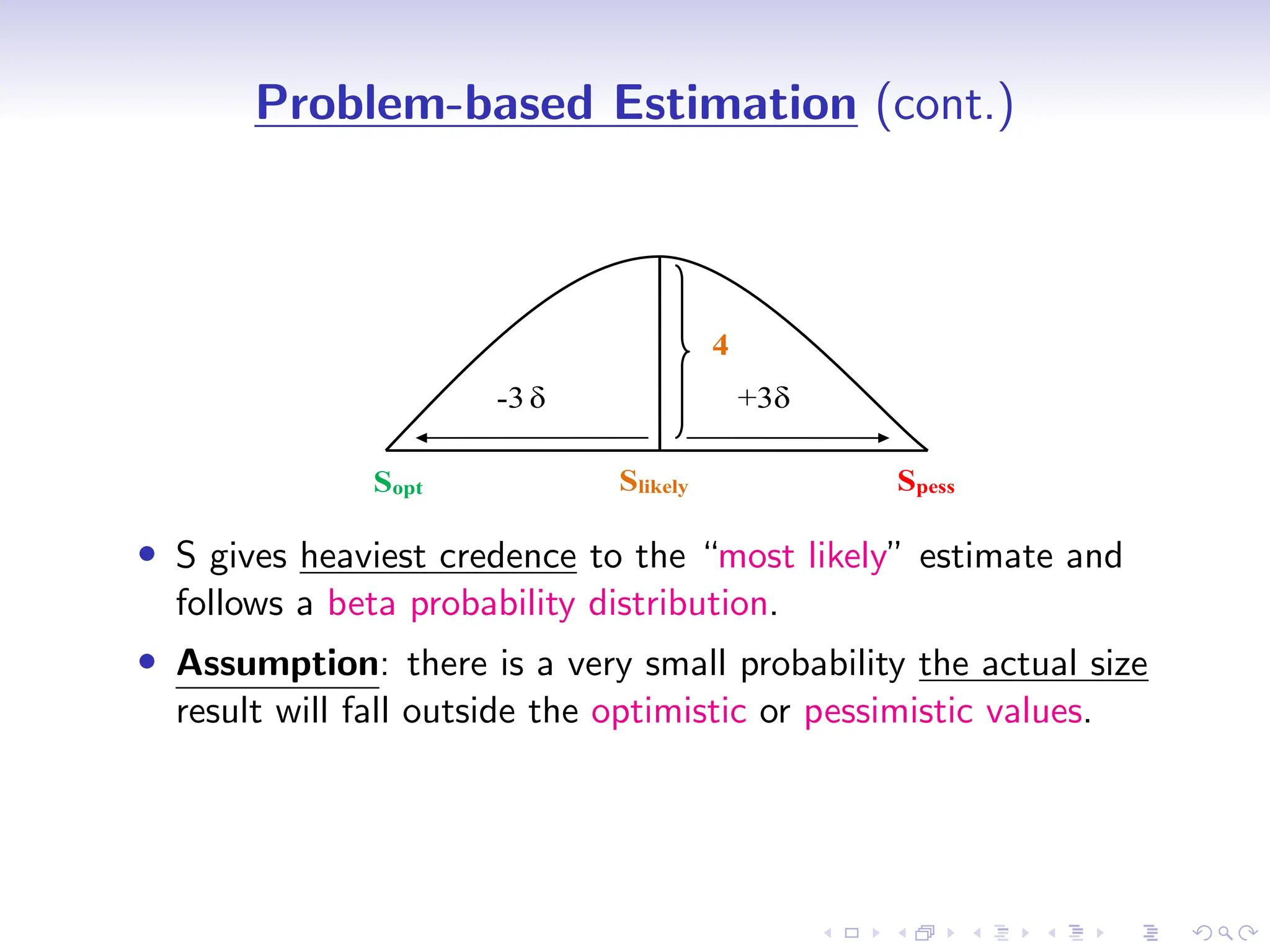
Problem-based Estimation (cont.)
SoptSlikely Spess
4
-3 +3
• S gives heaviest credence to the “most likely” estimate and
follows a beta probability distribution.
• Assumption: there is a very small probability the actual size
result will fall outside the optimistic or pessimistic values.
18.
D
r
a
f
t
Problem-based Estimation (cont.)
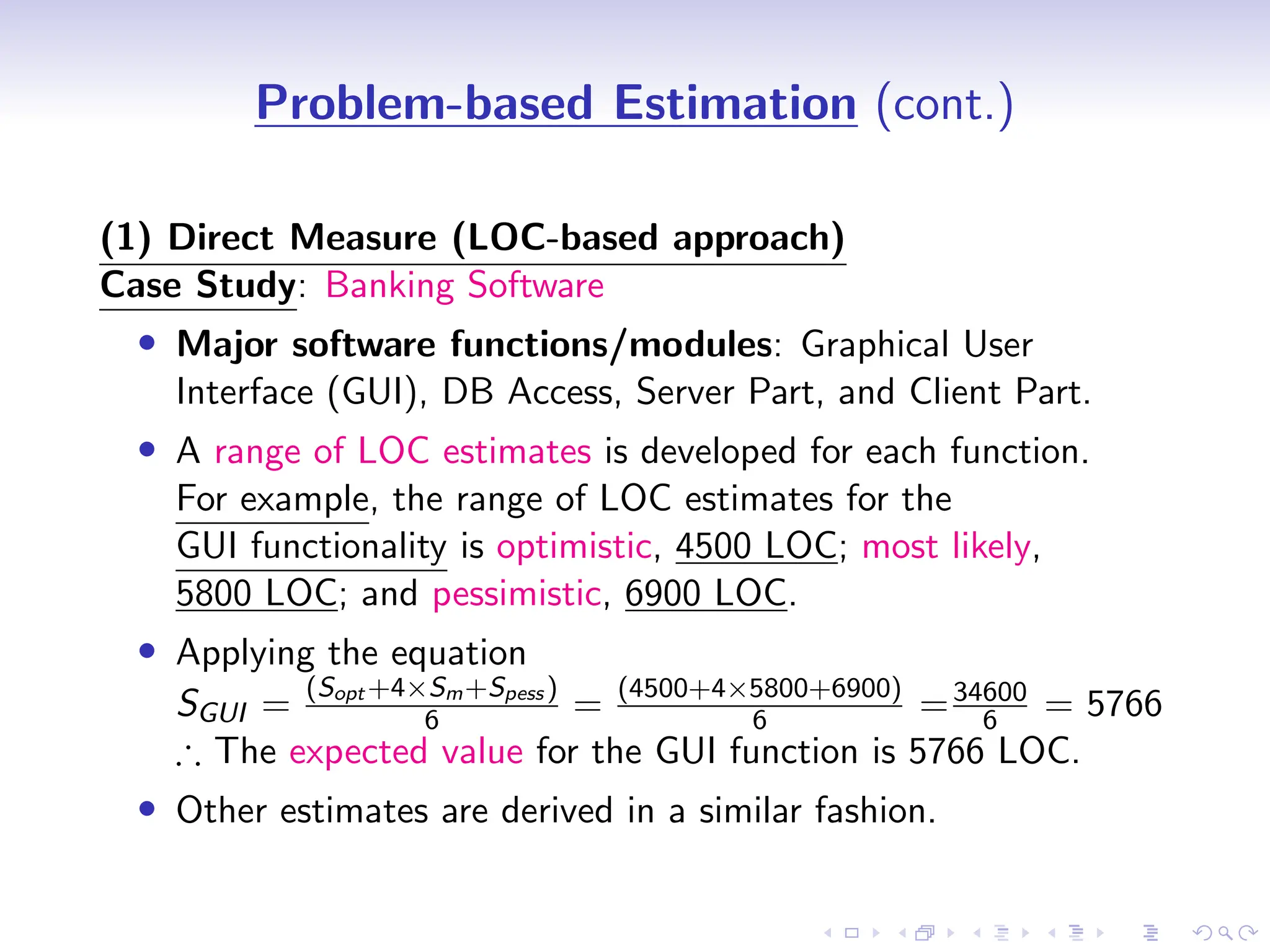
(1)Direct Measure (LOC-based approach)
Case Study: Banking Software
• Major software functions/modules: Graphical User
Interface (GUI), DB Access, Server Part, and Client Part.
• A range of LOC estimates is developed for each function.
For example, the range of LOC estimates for the
GUI functionality is optimistic, 4500 LOC; most likely,
5800 LOC; and pessimistic, 6900 LOC.
• Applying the equation
SGUI =
(Sopt +4×Sm+Spess )
6 = (4500+4×5800+6900)
6 =34600
6 = 5766
∴ The expected value for the GUI function is 5766 LOC.
• Other estimates are derived in a similar fashion.
19.
D
r
a
f
t
Problem-based Estimation (cont.)
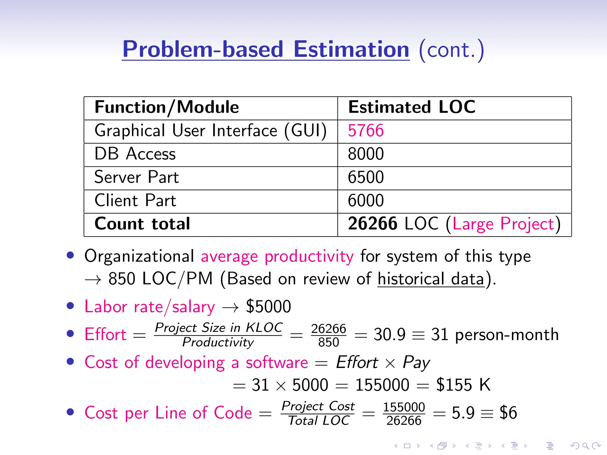
Function/ModuleEstimated LOC
Graphical User Interface (GUI) 5766
DB Access 8000
Server Part 6500
Client Part 6000
Count total 26266 LOC (Large Project)
• Organizational average productivity for system of this type
→ 850 LOC/PM (Based on review of historical data).
• Labor rate/salary → $5000
• Effort = Project Size in KLOC
Productivity = 26266
850 = 30.9 ≡ 31 person-month
• Cost of developing a software = Effort × Pay
= 31 × 5000 = 155000 = $155 K
• Cost per Line of Code = Project Cost
Total LOC = 155000
26266 = 5.9 ≡ $6
20.
D
r
a
f
t
Problem-based Estimation (cont.)
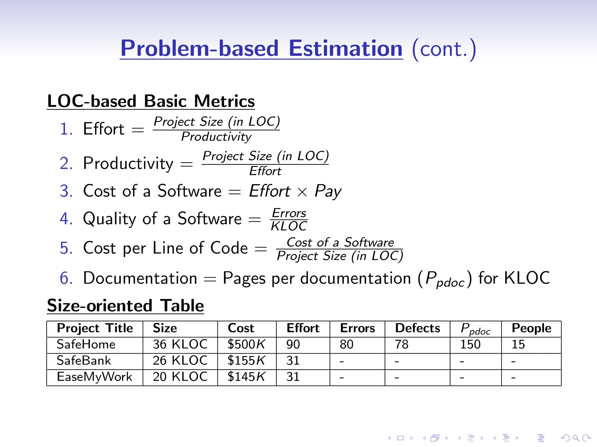
LOC-basedBasic Metrics
1. Effort = Project Size (in LOC)
Productivity
2. Productivity = Project Size (in LOC)
Effort
3. Cost of a Software = Effort × Pay
4. Quality of a Software = Errors
KLOC
5. Cost per Line of Code = Cost of a Software
Project Size (in LOC)
6. Documentation = Pages per documentation (Ppdoc) for KLOC
Size-oriented Table
Project Title Size Cost Effort Errors Defects Ppdoc People
SafeHome 36 KLOC $500K 90 80 78 150 15
SafeBank 26 KLOC $155K 31 - - - -
EaseMyWork 20 KLOC $145K 31 - - - -
21.
D
r
a
f
t
Problem-based Estimation (cont.)
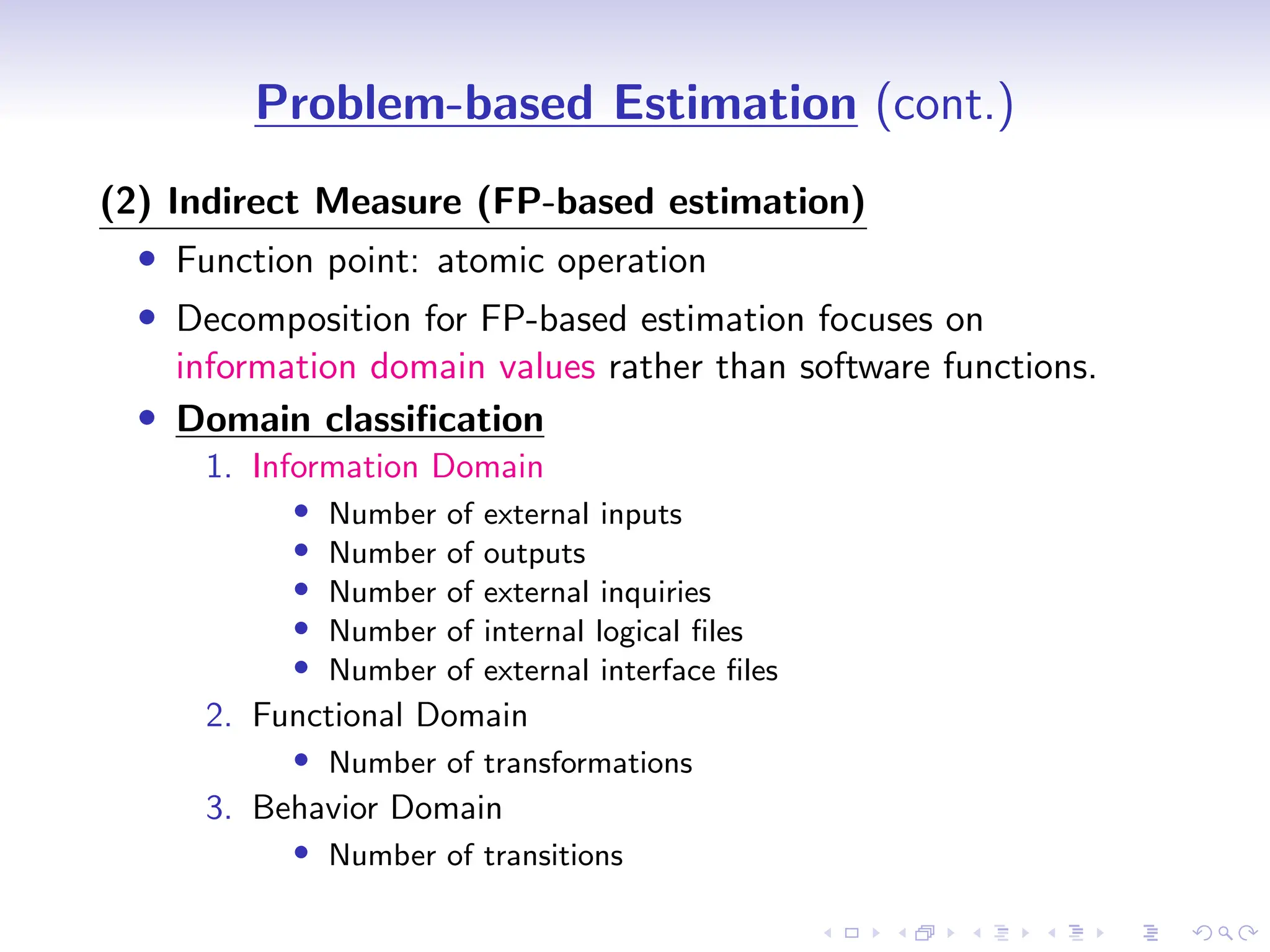
(2)Indirect Measure (FP-based estimation)
• Function point: atomic operation
• Decomposition for FP-based estimation focuses on
information domain values rather than software functions.
• Domain classification
1. Information Domain
• Number of external inputs
• Number of outputs
• Number of external inquiries
• Number of internal logical files
• Number of external interface files
2. Functional Domain
• Number of transformations
3. Behavior Domain
• Number of transitions
22.
D
r
a
f
t
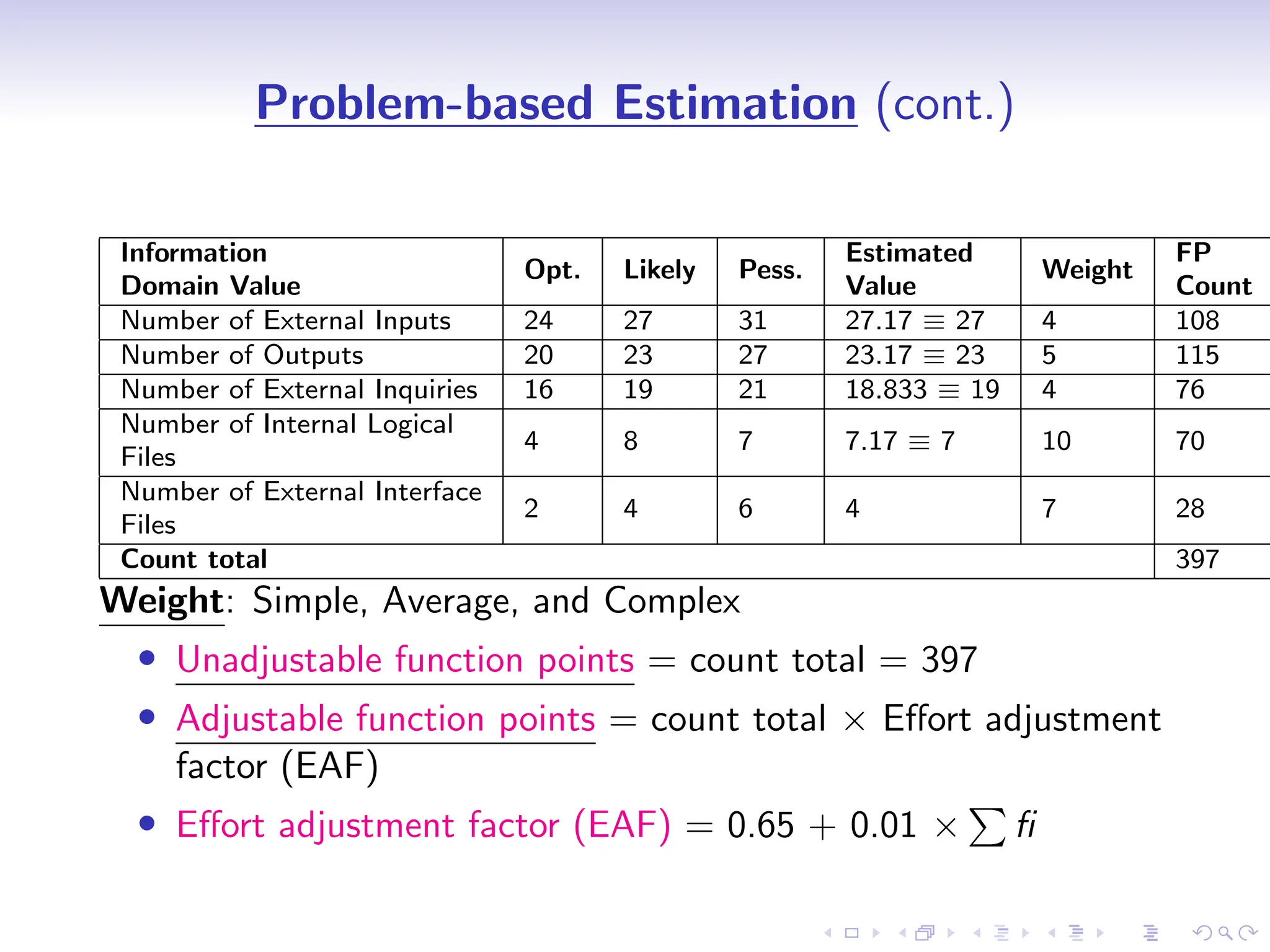
Problem-based Estimation (cont.)
Information
DomainValue
Opt. Likely Pess.
Estimated
Value
Weight
FP
Count
Number of External Inputs 24 27 31 27.17 ≡ 27 4 108
Number of Outputs 20 23 27 23.17 ≡ 23 5 115
Number of External Inquiries 16 19 21 18.833 ≡ 19 4 76
Number of Internal Logical
Files
4 8 7 7.17 ≡ 7 10 70
Number of External Interface
Files
2 4 6 4 7 28
Count total 397
Weight: Simple, Average, and Complex
• Unadjustable function points = count total = 397
• Adjustable function points = count total × Effort adjustment
factor (EAF)
• Effort adjustment factor (EAF) = 0.65 + 0.01 ×
P
fi
23.
D
r
a
f
t
Problem-based Estimation (cont.)
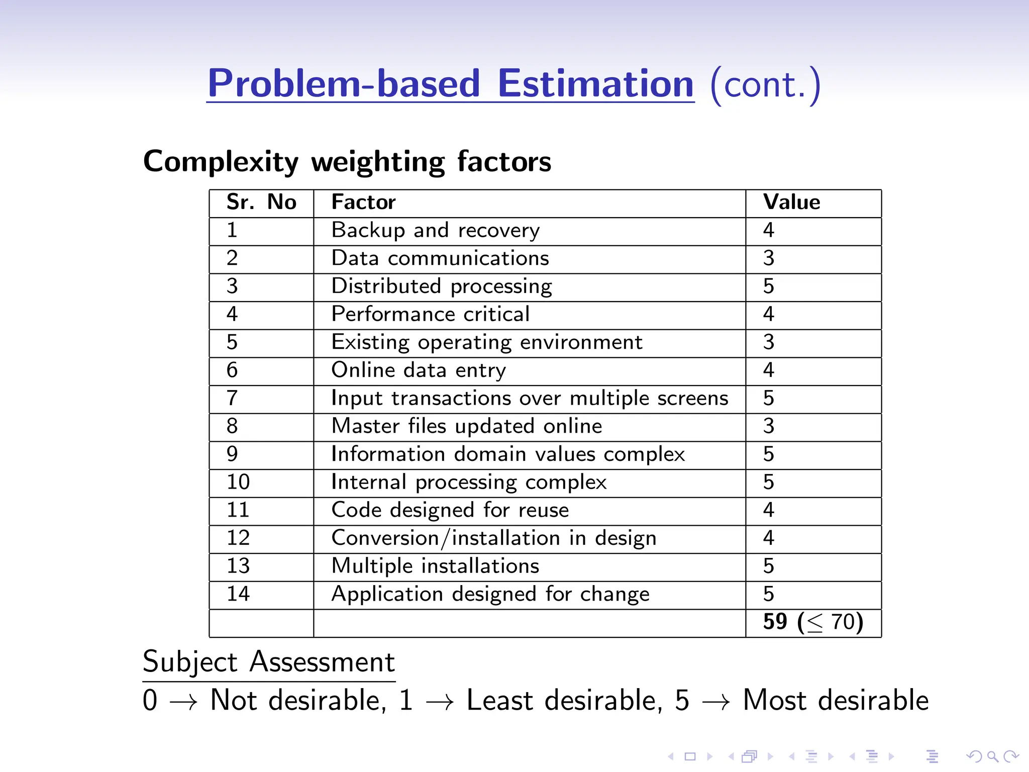
Complexityweighting factors
Sr. No Factor Value
1 Backup and recovery 4
2 Data communications 3
3 Distributed processing 5
4 Performance critical 4
5 Existing operating environment 3
6 Online data entry 4
7 Input transactions over multiple screens 5
8 Master files updated online 3
9 Information domain values complex 5
10 Internal processing complex 5
11 Code designed for reuse 4
12 Conversion/installation in design 4
13 Multiple installations 5
14 Application designed for change 5
59 (≤ 70)
Subject Assessment
0 → Not desirable, 1 → Least desirable, 5 → Most desirable
24.
D
r
a
f
t
Problem-based Estimation (cont.)
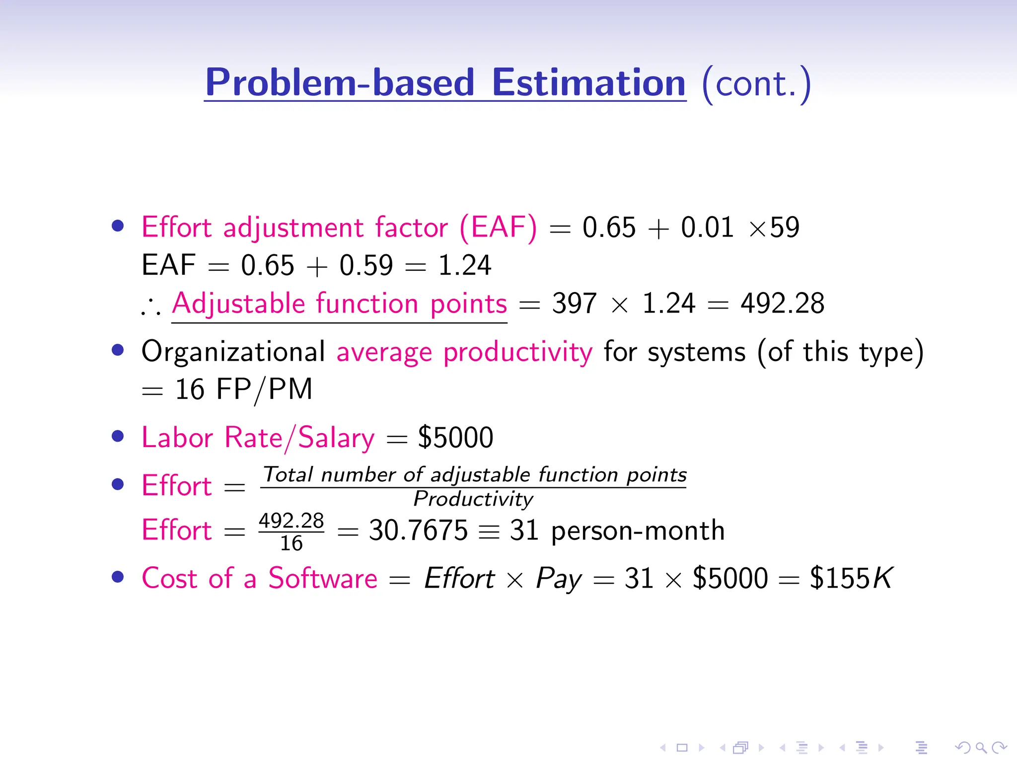
•Effort adjustment factor (EAF) = 0.65 + 0.01 ×59
EAF = 0.65 + 0.59 = 1.24
∴ Adjustable function points = 397 × 1.24 = 492.28
• Organizational average productivity for systems (of this type)
= 16 FP/PM
• Labor Rate/Salary = $5000
• Effort = Total number of adjustable function points
Productivity
Effort = 492.28
16 = 30.7675 ≡ 31 person-month
• Cost of a Software = Effort × Pay = 31 × $5000 = $155K
25.
D
r
a
f
t
Problem-based Estimation (cont.)
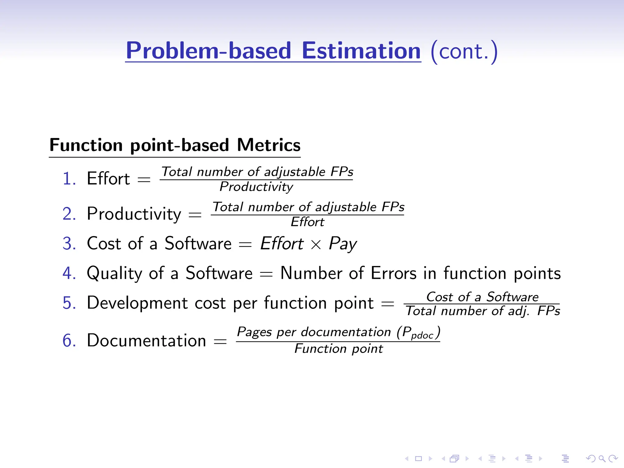
Functionpoint-based Metrics
1. Effort = Total number of adjustable FPs
Productivity
2. Productivity = Total number of adjustable FPs
Effort
3. Cost of a Software = Effort × Pay
4. Quality of a Software = Number of Errors in function points
5. Development cost per function point = Cost of a Software
Total number of adj. FPs
6. Documentation =
Pages per documentation (Ppdoc )
Function point
26.
D
r
a
f
t
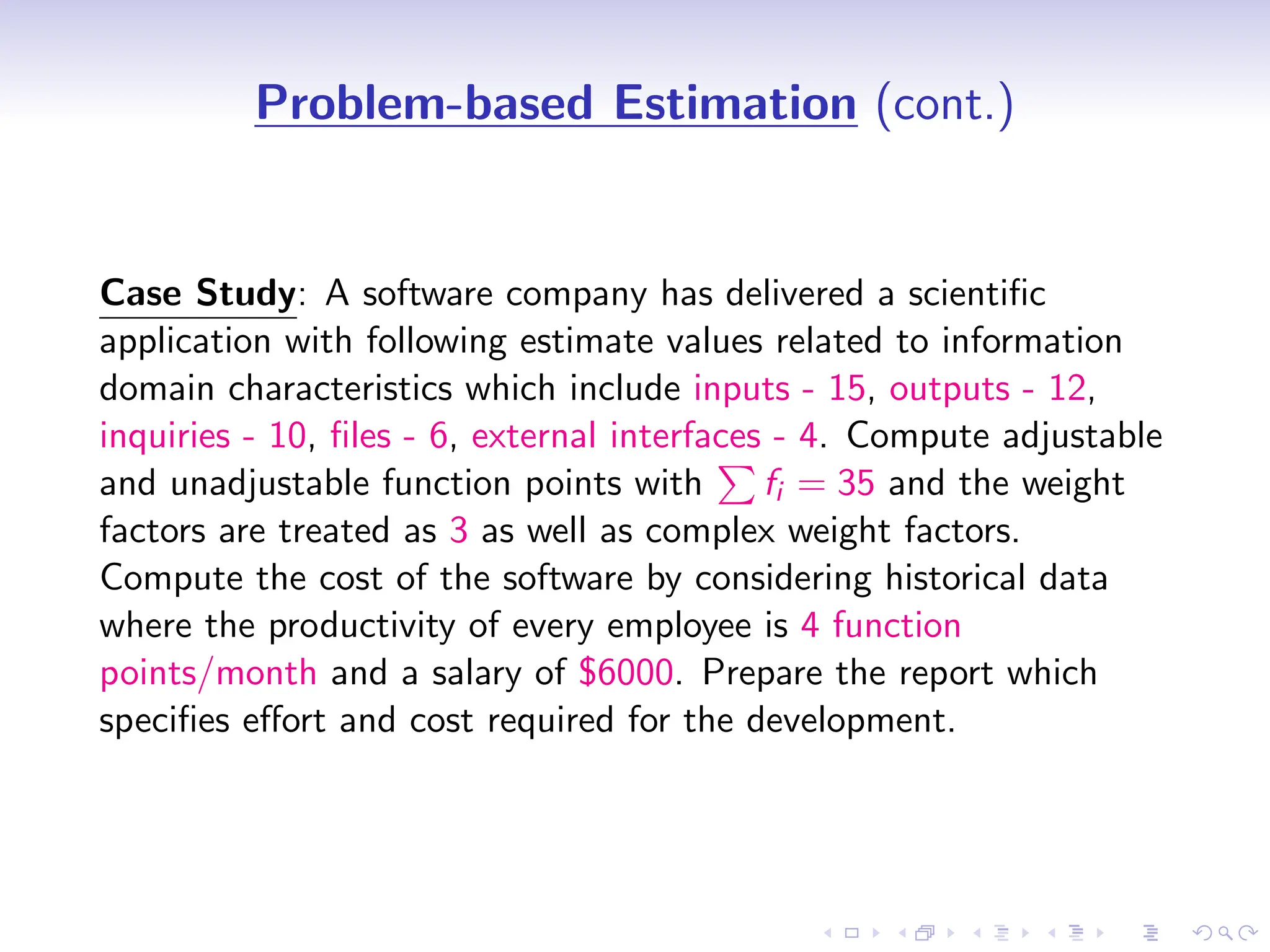
Problem-based Estimation (cont.)
CaseStudy: A software company has delivered a scientific
application with following estimate values related to information
domain characteristics which include inputs - 15, outputs - 12,
inquiries - 10, files - 6, external interfaces - 4. Compute adjustable
and unadjustable function points with
P
fi = 35 and the weight
factors are treated as 3 as well as complex weight factors.
Compute the cost of the software by considering historical data
where the productivity of every employee is 4 function
points/month and a salary of $6000. Prepare the report which
specifies effort and cost required for the development.
27.
D
r
a
f
t
Problem-based Estimation (cont.)
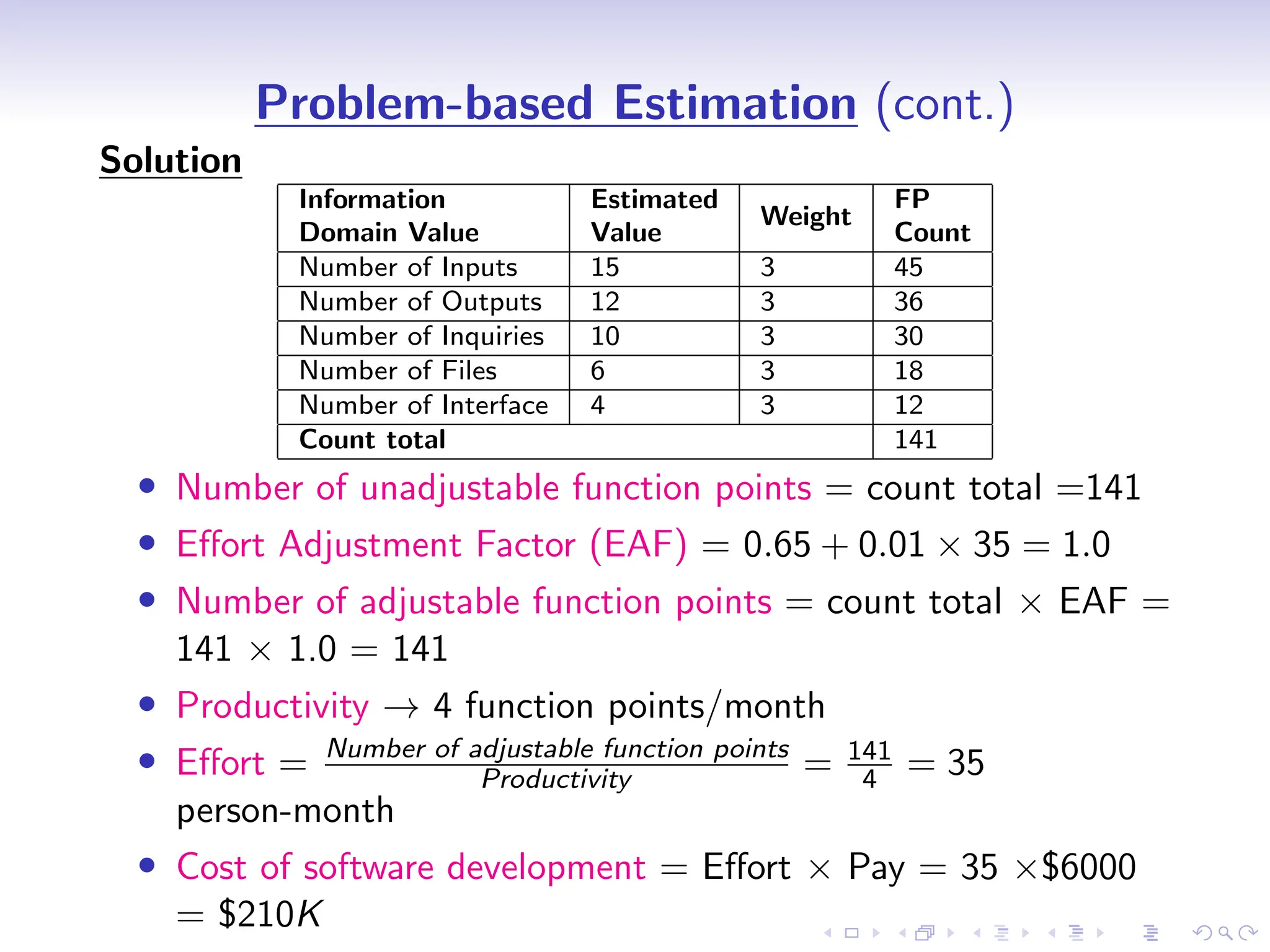
Solution
Information
DomainValue
Estimated
Value
Weight
FP
Count
Number of Inputs 15 3 45
Number of Outputs 12 3 36
Number of Inquiries 10 3 30
Number of Files 6 3 18
Number of Interface 4 3 12
Count total 141
• Number of unadjustable function points = count total =141
• Effort Adjustment Factor (EAF) = 0.65 + 0.01 × 35 = 1.0
• Number of adjustable function points = count total × EAF =
141 × 1.0 = 141
• Productivity → 4 function points/month
• Effort = Number of adjustable function points
Productivity = 141
4 = 35
person-month
• Cost of software development = Effort × Pay = 35 ×$6000
= $210K
28.
D
r
a
f
t
Process-based Estimation
• Idea:base the estimate on the process that will be used for
software development.
• The process is decomposed into a relatively small set of tasks
and the effort required to accomplish each task is estimated.
• Begins with a description of software functions obtained from
the project scope.
• A series of framework activities must be performed for each
function.
29.
D
r
a
f
t
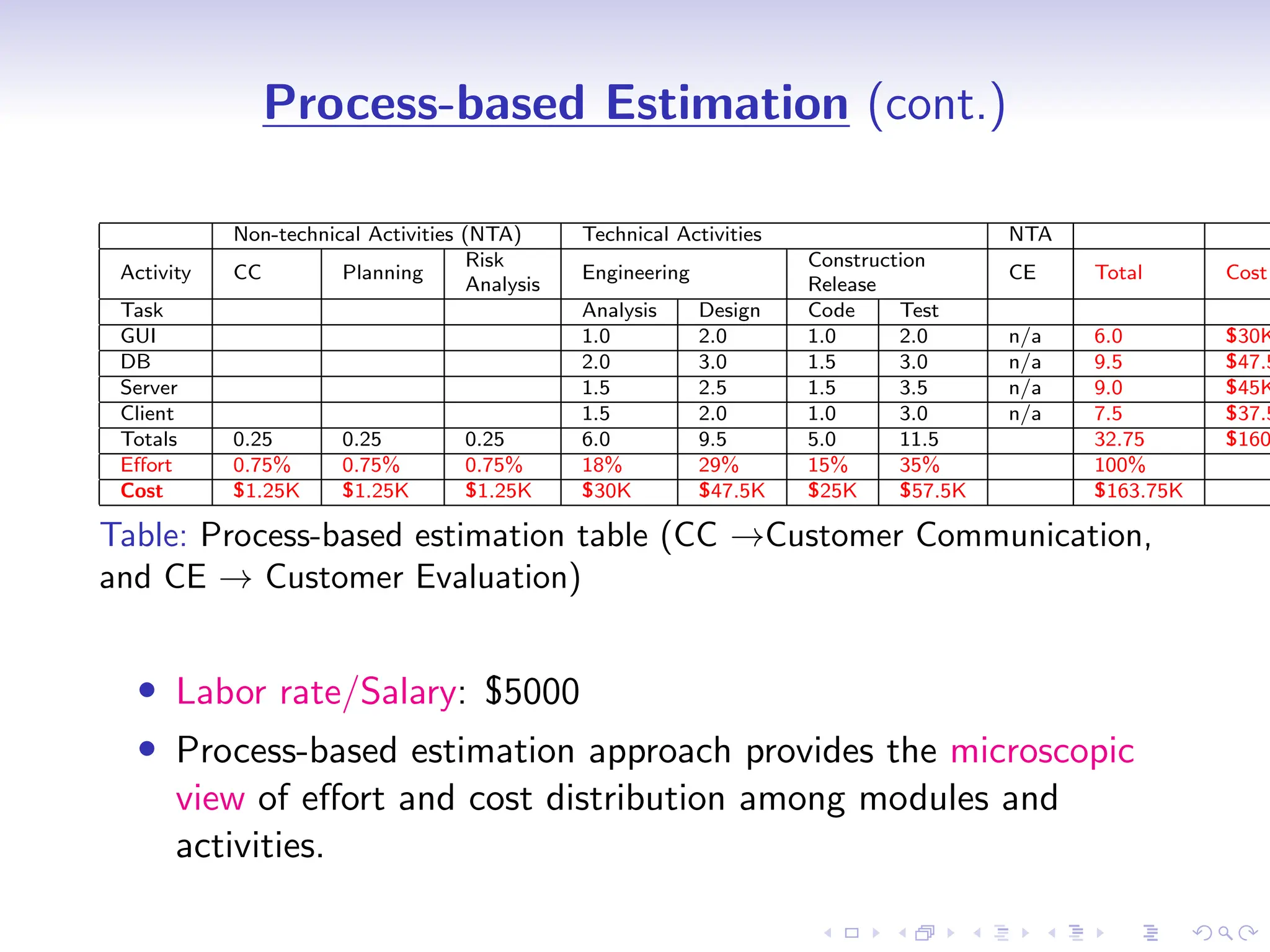
Process-based Estimation (cont.)
Non-technicalActivities (NTA) Technical Activities NTA
Activity CC Planning
Risk
Analysis
Engineering
Construction
Release
CE Total Cost
Task Analysis Design Code Test
GUI 1.0 2.0 1.0 2.0 n/a 6.0 $30K
DB 2.0 3.0 1.5 3.0 n/a 9.5 $47.5
Server 1.5 2.5 1.5 3.5 n/a 9.0 $45K
Client 1.5 2.0 1.0 3.0 n/a 7.5 $37.5
Totals 0.25 0.25 0.25 6.0 9.5 5.0 11.5 32.75 $160
Effort 0.75% 0.75% 0.75% 18% 29% 15% 35% 100%
Cost $1.25K $1.25K $1.25K $30K $47.5K $25K $57.5K $163.75K
Table: Process-based estimation table (CC →Customer Communication,
and CE → Customer Evaluation)
• Labor rate/Salary: $5000
• Process-based estimation approach provides the microscopic
view of effort and cost distribution among modules and
activities.
30.
D
r
a
f
t
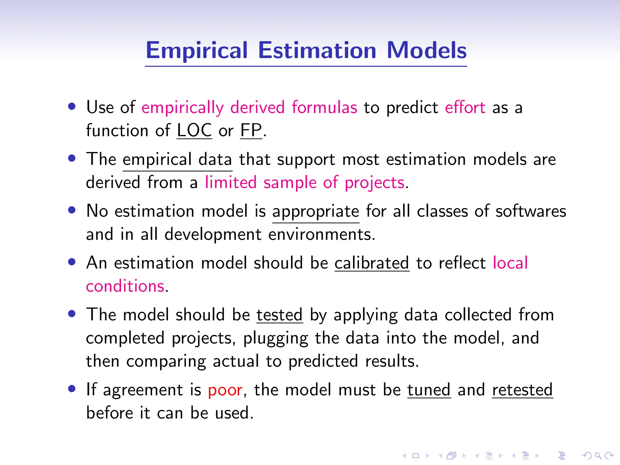
Empirical Estimation Models
•Use of empirically derived formulas to predict effort as a
function of LOC or FP.
• The empirical data that support most estimation models are
derived from a limited sample of projects.
• No estimation model is appropriate for all classes of softwares
and in all development environments.
• An estimation model should be calibrated to reflect local
conditions.
• The model should be tested by applying data collected from
completed projects, plugging the data into the model, and
then comparing actual to predicted results.
• If agreement is poor, the model must be tuned and retested
before it can be used.
31.
D
r
a
f
t
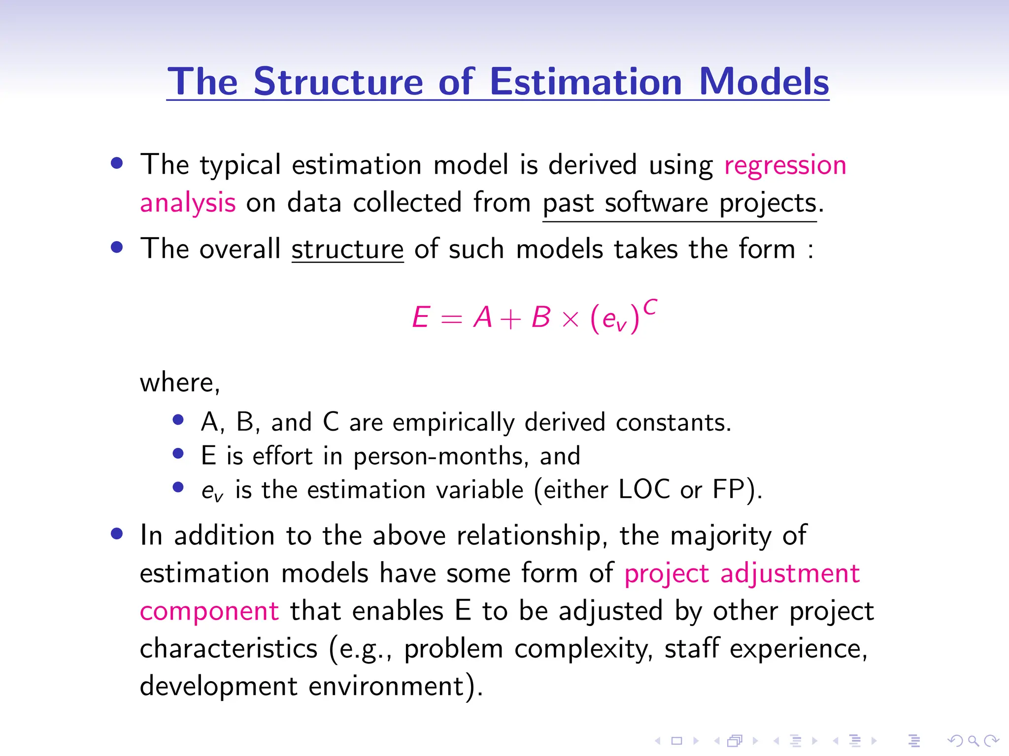
The Structure ofEstimation Models
• The typical estimation model is derived using regression
analysis on data collected from past software projects.
• The overall structure of such models takes the form :
E = A + B × (ev )C
where,
• A, B, and C are empirically derived constants.
• E is effort in person-months, and
• ev is the estimation variable (either LOC or FP).
• In addition to the above relationship, the majority of
estimation models have some form of project adjustment
component that enables E to be adjusted by other project
characteristics (e.g., problem complexity, staff experience,
development environment).
32.
D
r
a
f
t
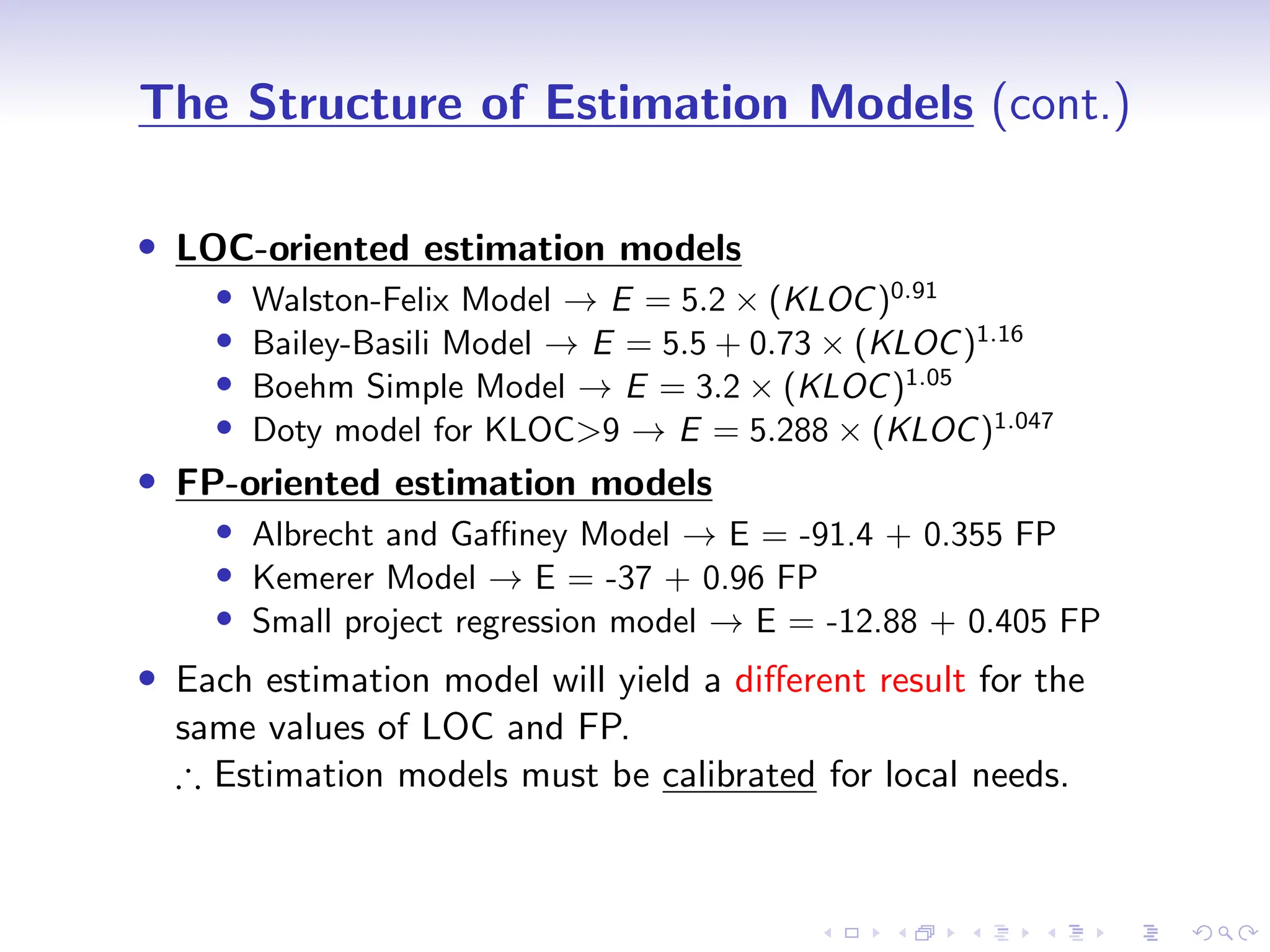
The Structure ofEstimation Models (cont.)
• LOC-oriented estimation models
• Walston-Felix Model → E = 5.2 × (KLOC)0.91
• Bailey-Basili Model → E = 5.5 + 0.73 × (KLOC)1.16
• Boehm Simple Model → E = 3.2 × (KLOC)1.05
• Doty model for KLOC>9 → E = 5.288 × (KLOC)1.047
• FP-oriented estimation models
• Albrecht and Gaffiney Model → E = -91.4 + 0.355 FP
• Kemerer Model → E = -37 + 0.96 FP
• Small project regression model → E = -12.88 + 0.405 FP
• Each estimation model will yield a different result for the
same values of LOC and FP.
∴ Estimation models must be calibrated for local needs.
33.
D
r
a
f
t
The COCOMO Model
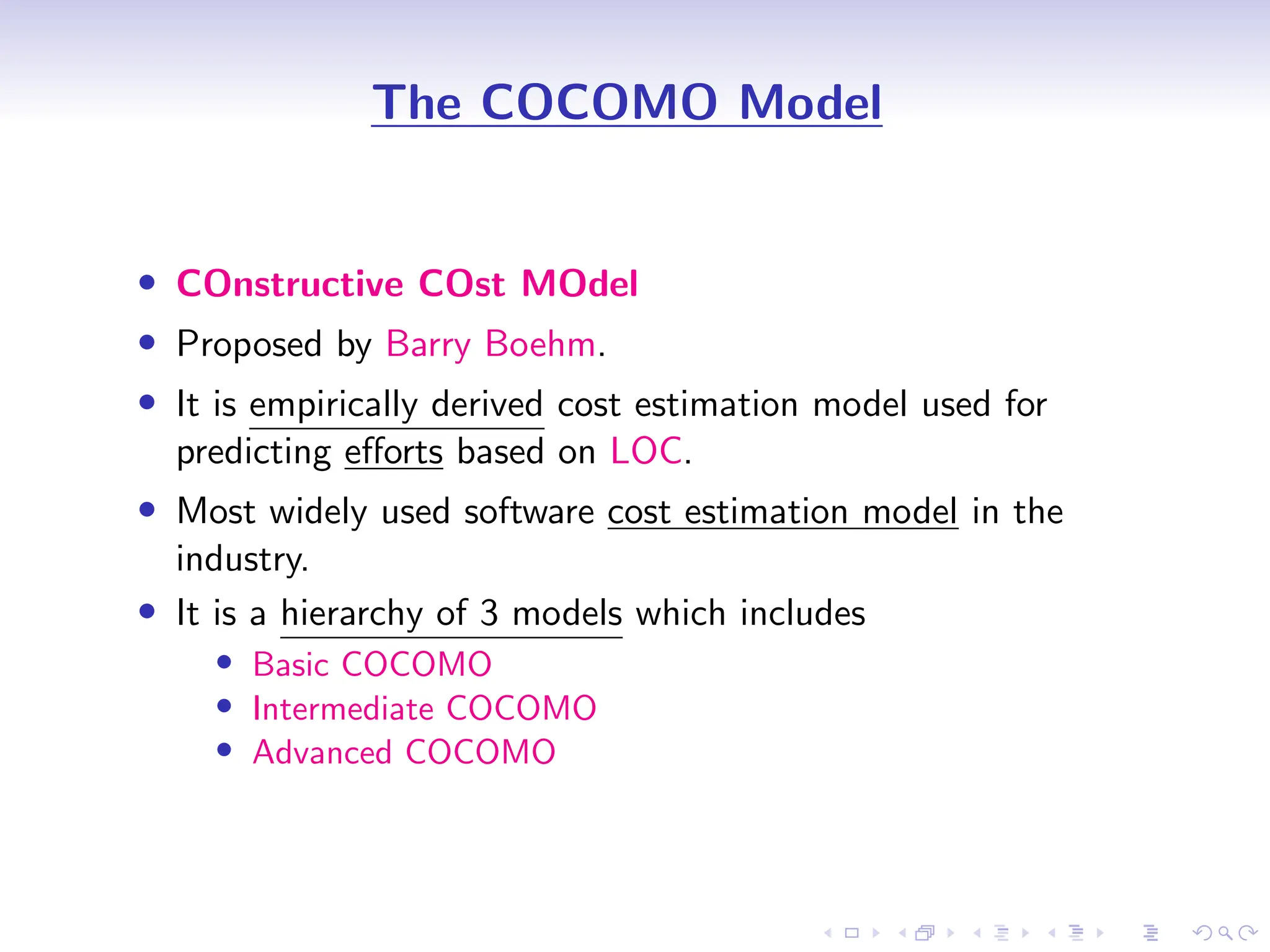
•COnstructive COst MOdel
• Proposed by Barry Boehm.
• It is empirically derived cost estimation model used for
predicting efforts based on LOC.
• Most widely used software cost estimation model in the
industry.
• It is a hierarchy of 3 models which includes
• Basic COCOMO
• Intermediate COCOMO
• Advanced COCOMO
34.
D
r
a
f
t
The COCOMO Model(cont.)
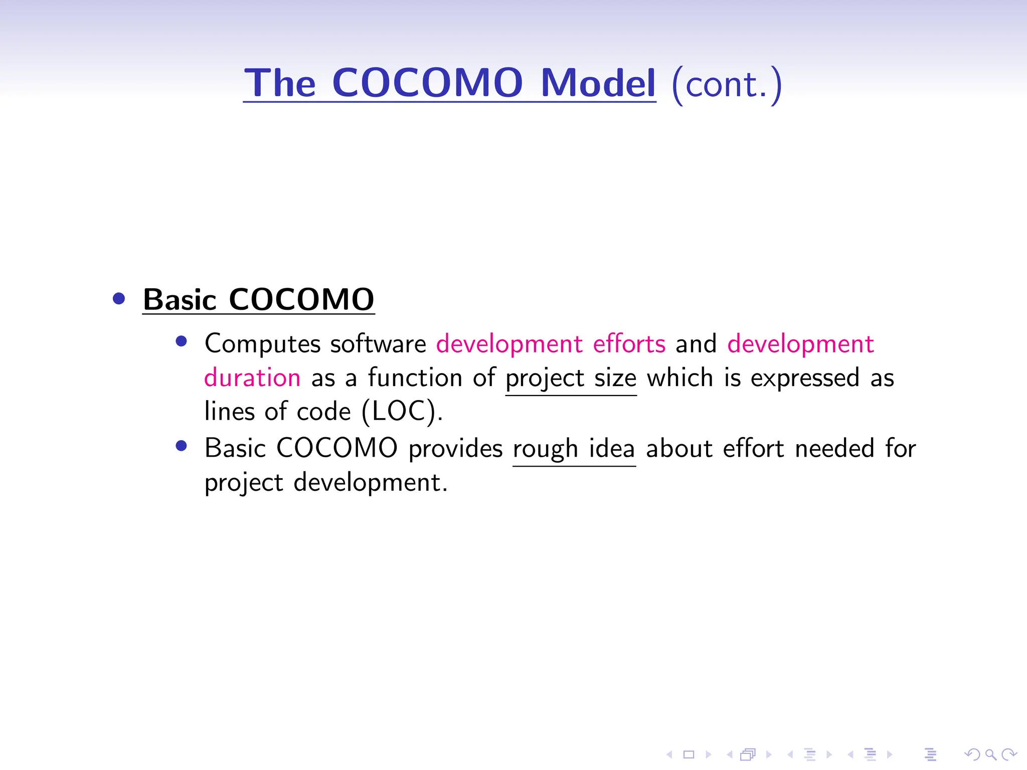
• Basic COCOMO
• Computes software development efforts and development
duration as a function of project size which is expressed as
lines of code (LOC).
• Basic COCOMO provides rough idea about effort needed for
project development.
35.
D
r
a
f
t
The COCOMO Model(cont.)
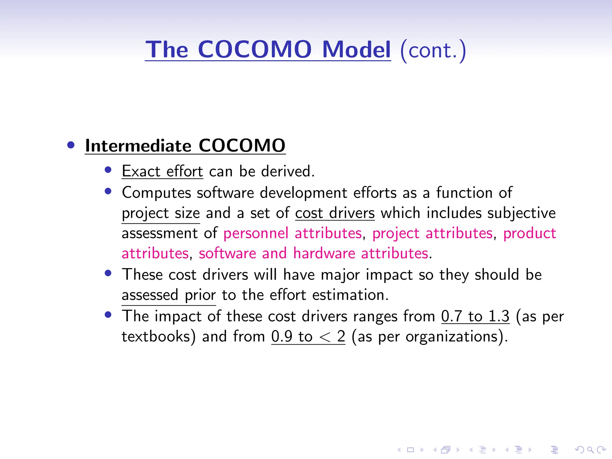
• Intermediate COCOMO
• Exact effort can be derived.
• Computes software development efforts as a function of
project size and a set of cost drivers which includes subjective
assessment of personnel attributes, project attributes, product
attributes, software and hardware attributes.
• These cost drivers will have major impact so they should be
assessed prior to the effort estimation.
• The impact of these cost drivers ranges from 0.7 to 1.3 (as per
textbooks) and from 0.9 to < 2 (as per organizations).
36.
D
r
a
f
t
The COCOMO Model(cont.)
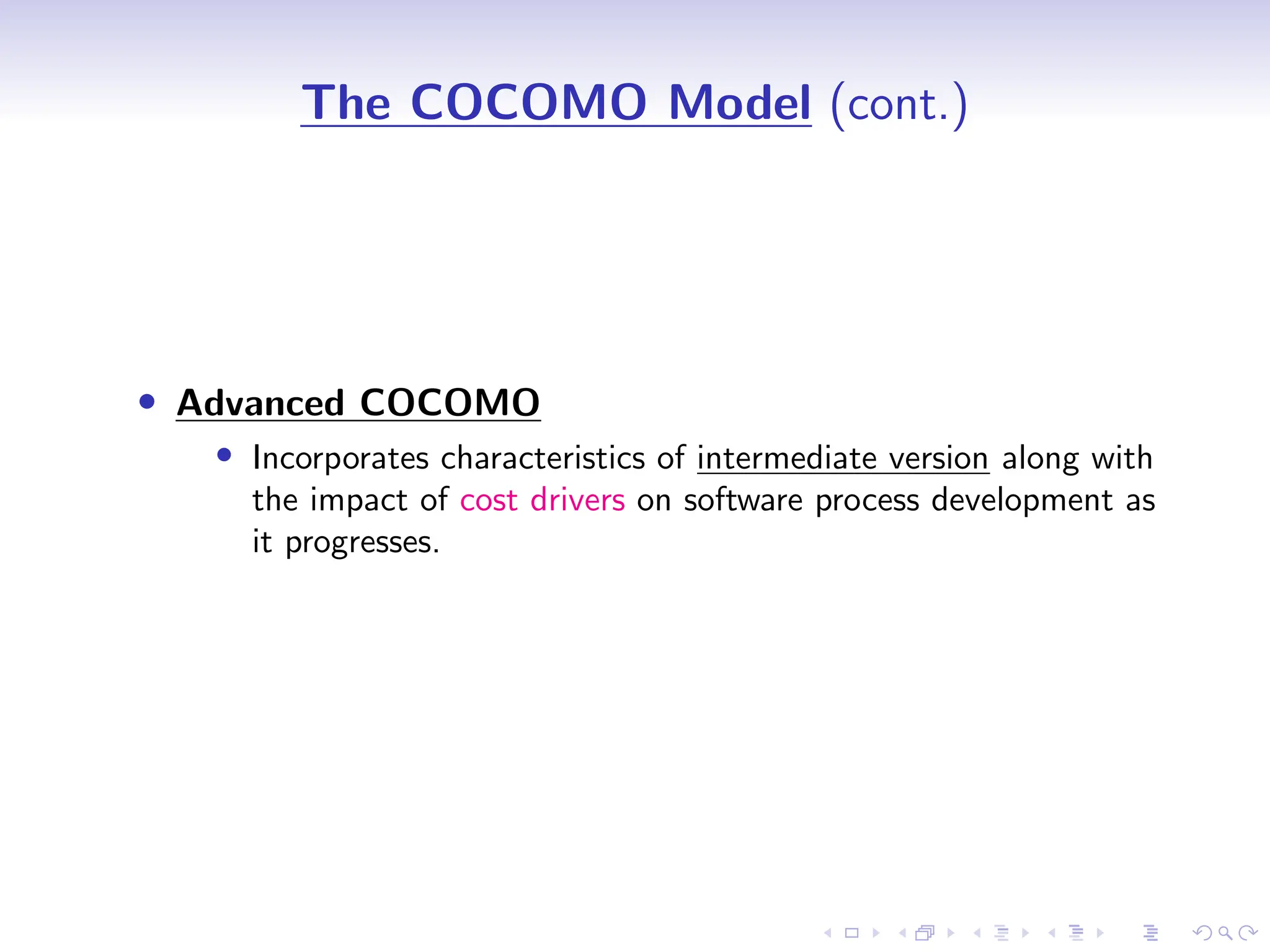
• Advanced COCOMO
• Incorporates characteristics of intermediate version along with
the impact of cost drivers on software process development as
it progresses.
37.
D
r
a
f
t
The COCOMO Model(cont.)
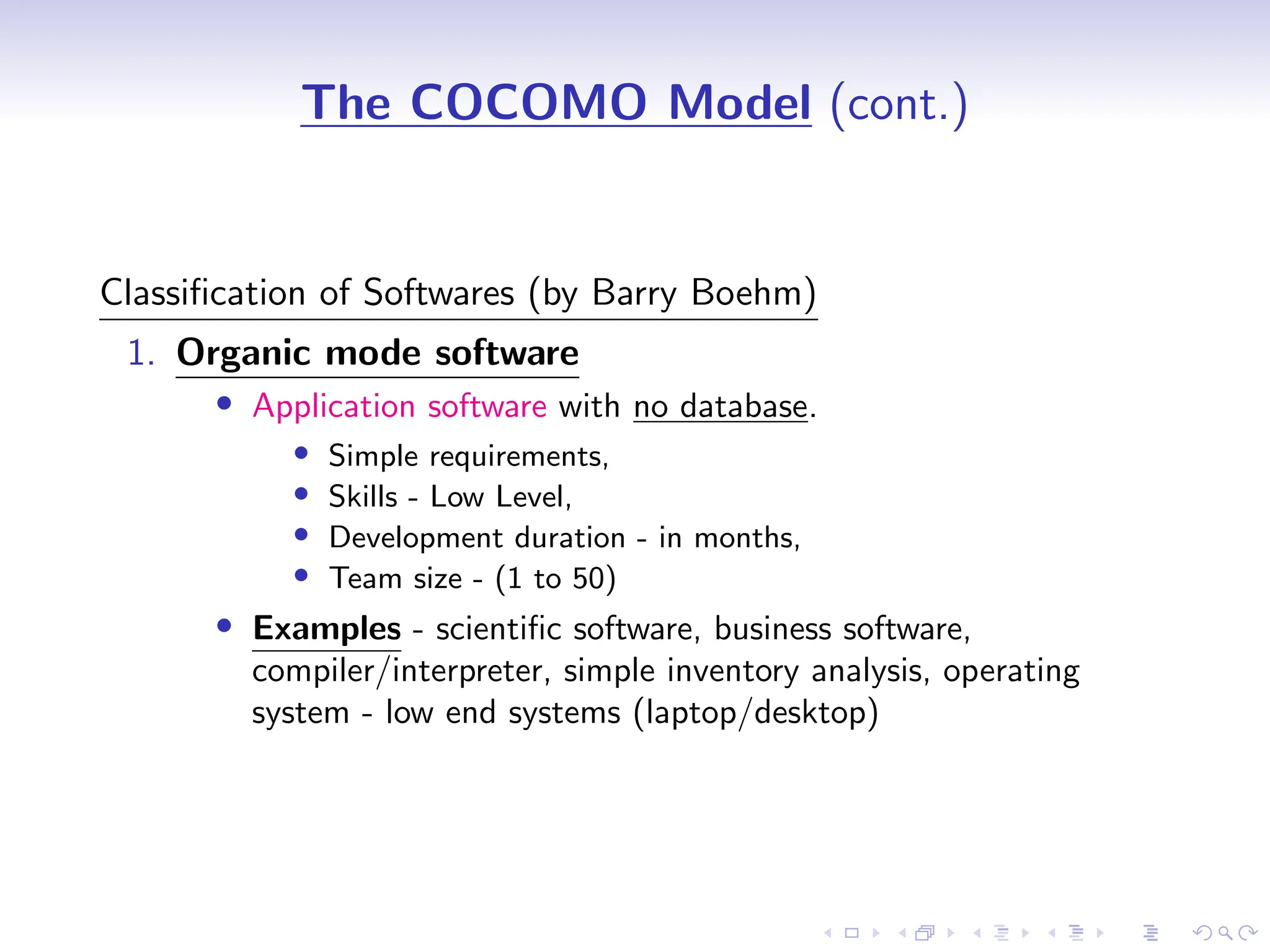
Classification of Softwares (by Barry Boehm)
1. Organic mode software
• Application software with no database.
• Simple requirements,
• Skills - Low Level,
• Development duration - in months,
• Team size - (1 to 50)
• Examples - scientific software, business software,
compiler/interpreter, simple inventory analysis, operating
system - low end systems (laptop/desktop)
38.
D
r
a
f
t
The COCOMO Model(cont.)
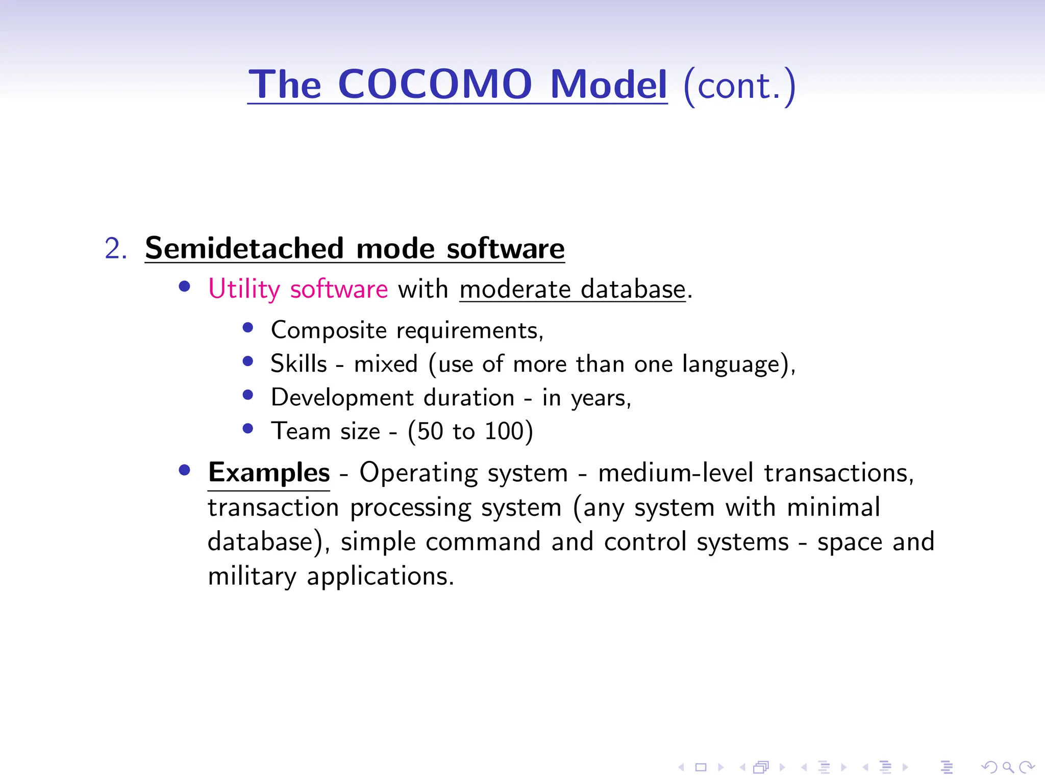
2. Semidetached mode software
• Utility software with moderate database.
• Composite requirements,
• Skills - mixed (use of more than one language),
• Development duration - in years,
• Team size - (50 to 100)
• Examples - Operating system - medium-level transactions,
transaction processing system (any system with minimal
database), simple command and control systems - space and
military applications.
39.
D
r
a
f
t
The COCOMO Model(cont.)
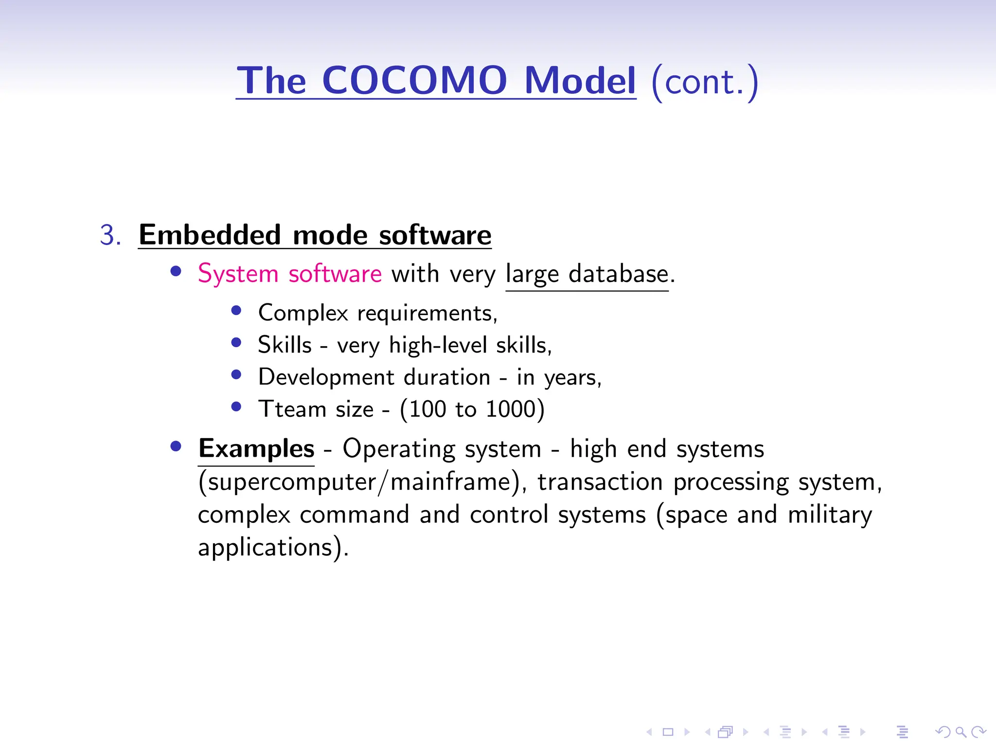
3. Embedded mode software
• System software with very large database.
• Complex requirements,
• Skills - very high-level skills,
• Development duration - in years,
• Tteam size - (100 to 1000)
• Examples - Operating system - high end systems
(supercomputer/mainframe), transaction processing system,
complex command and control systems (space and military
applications).
40.
D
r
a
f
t
The COCOMO Model(cont.)
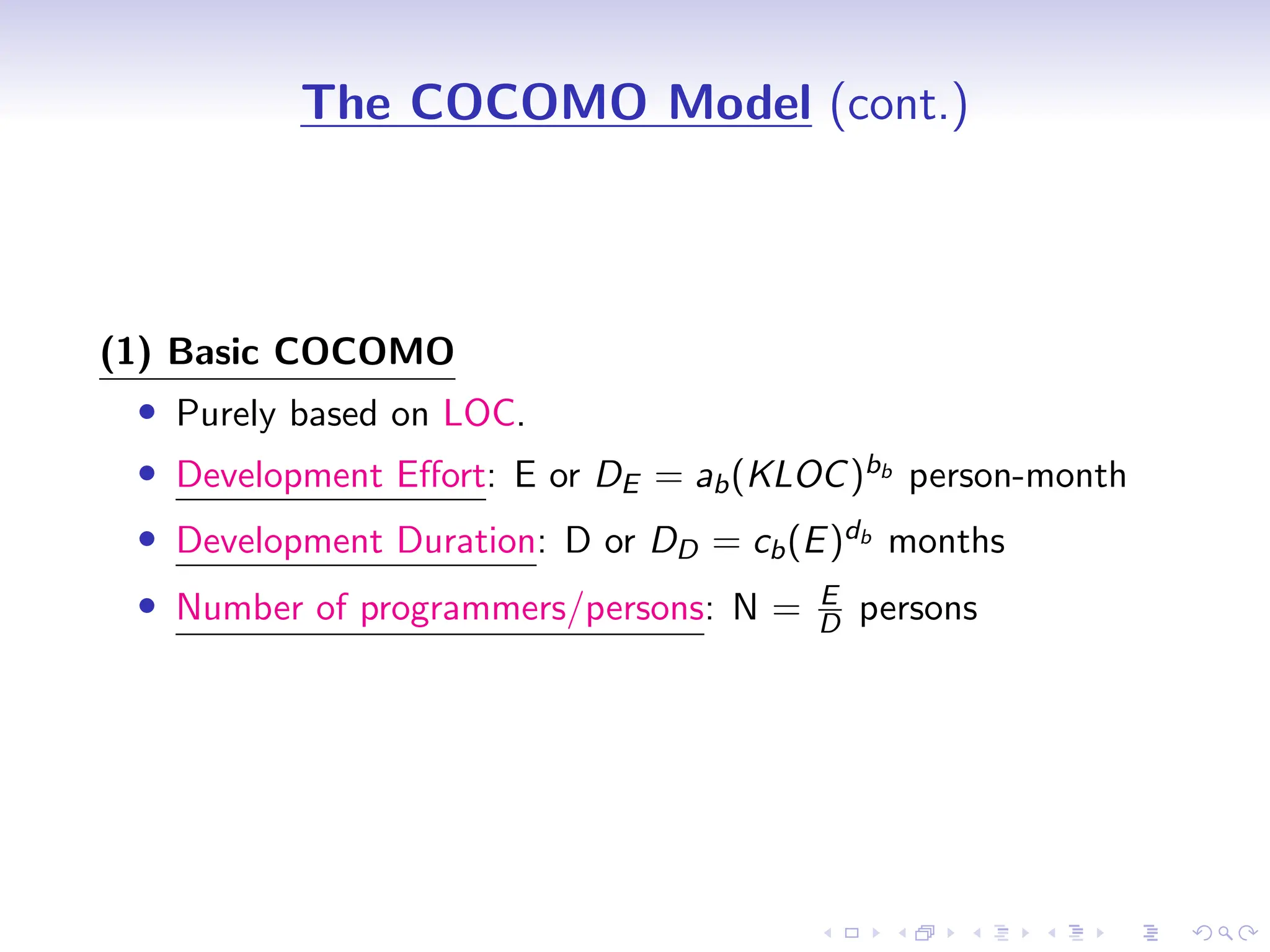
(1) Basic COCOMO
• Purely based on LOC.
• Development Effort: E or DE = ab(KLOC)bb person-month
• Development Duration: D or DD = cb(E)db months
• Number of programmers/persons: N = E
D persons
41.
D
r
a
f
t
The COCOMO Model(cont.)
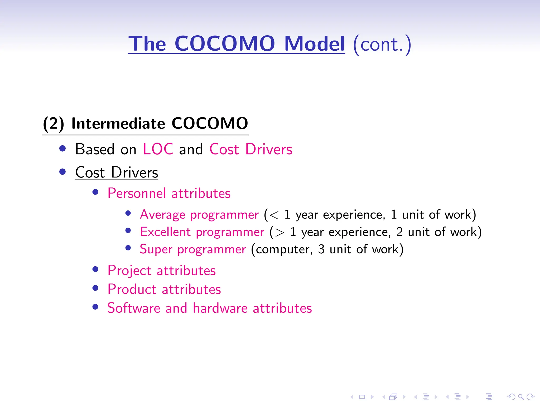
(2) Intermediate COCOMO
• Based on LOC and Cost Drivers
• Cost Drivers
• Personnel attributes
• Average programmer (< 1 year experience, 1 unit of work)
• Excellent programmer (> 1 year experience, 2 unit of work)
• Super programmer (computer, 3 unit of work)
• Project attributes
• Product attributes
• Software and hardware attributes
42.
D
r
a
f
t
The COCOMO Model(cont.)
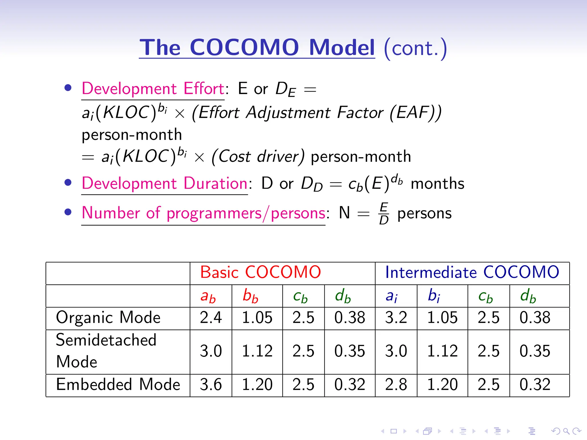
• Development Effort: E or DE =
ai (KLOC)bi × (Effort Adjustment Factor (EAF))
person-month
= ai (KLOC)bi × (Cost driver) person-month
• Development Duration: D or DD = cb(E)db months
• Number of programmers/persons: N = E
D persons
Basic COCOMO Intermediate COCOMO
ab bb cb db ai bi cb db
Organic Mode 2.4 1.05 2.5 0.38 3.2 1.05 2.5 0.38
Semidetached
Mode
3.0 1.12 2.5 0.35 3.0 1.12 2.5 0.35
Embedded Mode 3.6 1.20 2.5 0.32 2.8 1.20 2.5 0.32
43.
D
r
a
f
t
The COCOMO Model(cont.)
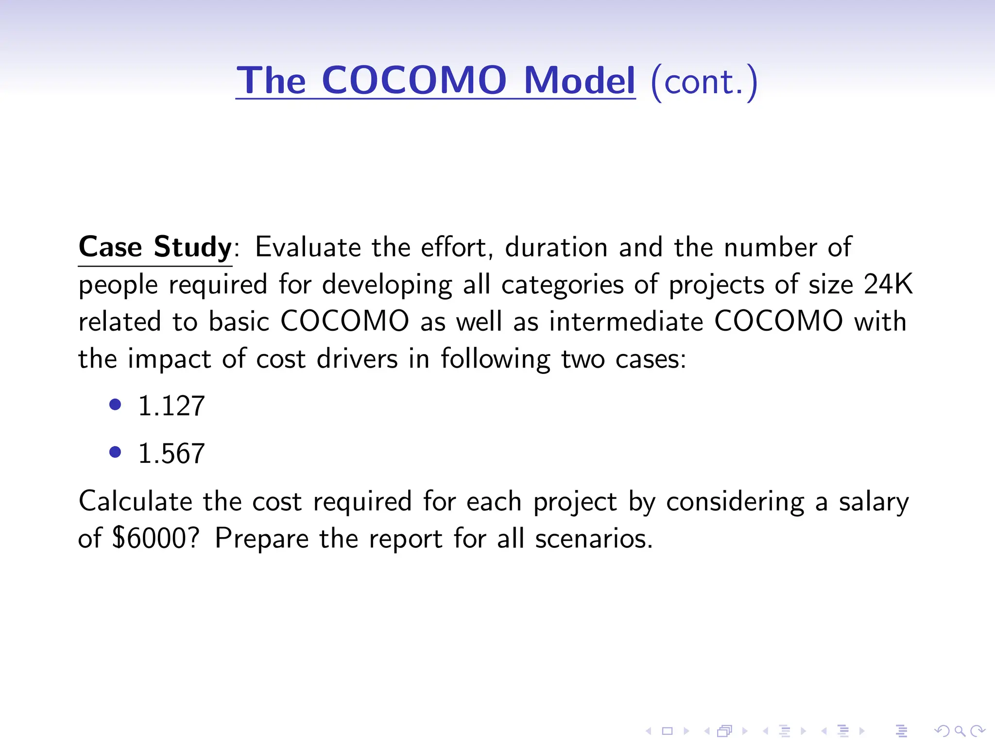
Case Study: Evaluate the effort, duration and the number of
people required for developing all categories of projects of size 24K
related to basic COCOMO as well as intermediate COCOMO with
the impact of cost drivers in following two cases:
• 1.127
• 1.567
Calculate the cost required for each project by considering a salary
of $6000? Prepare the report for all scenarios.
44.
D
r
a
f
t
The COCOMO Model(cont.)
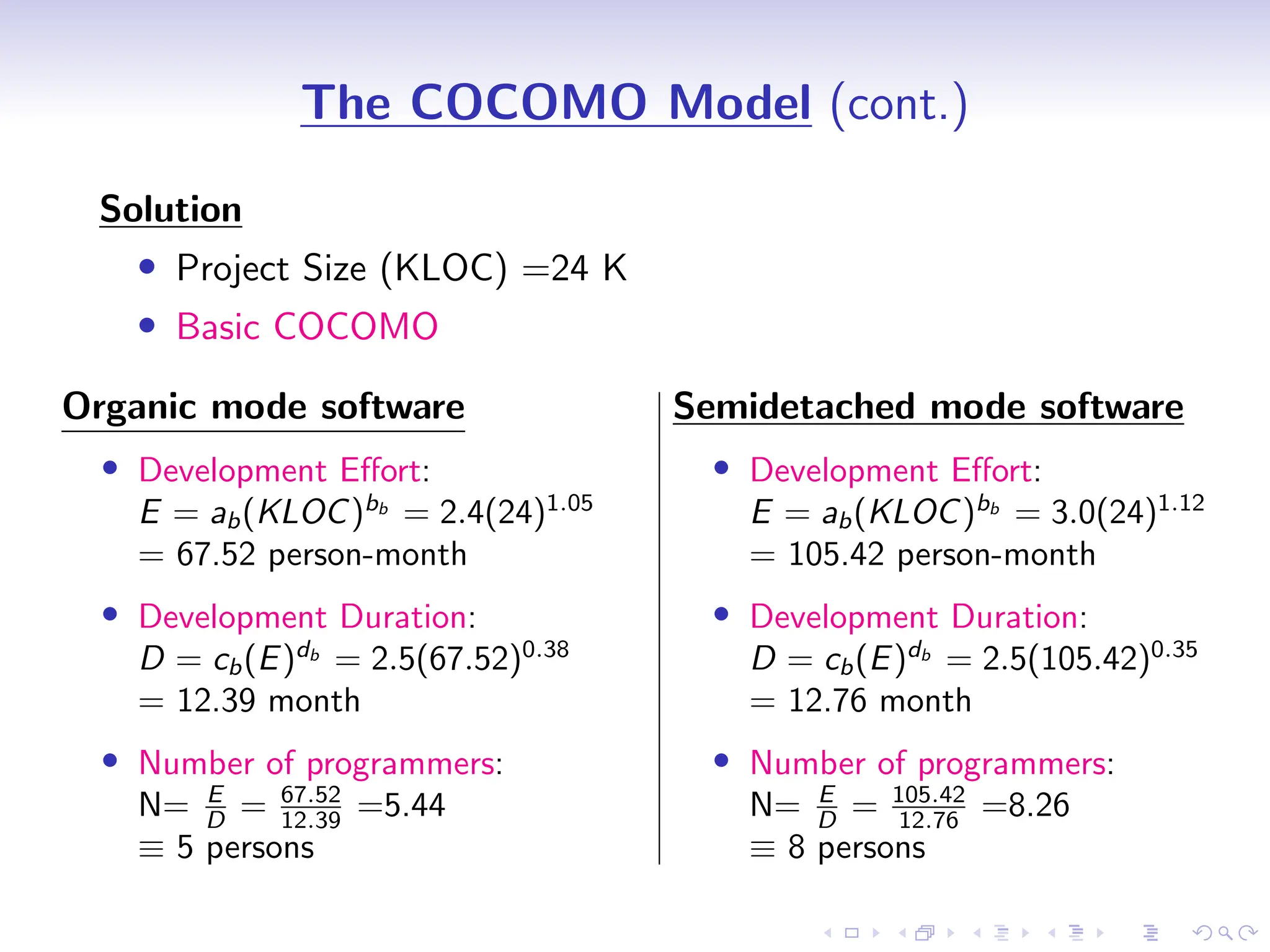
Solution
• Project Size (KLOC) =24 K
• Basic COCOMO
Organic mode software
• Development Effort:
E = ab(KLOC)bb
= 2.4(24)1.05
= 67.52 person-month
• Development Duration:
D = cb(E)db
= 2.5(67.52)0.38
= 12.39 month
• Number of programmers:
N= E
D = 67.52
12.39 =5.44
≡ 5 persons
Semidetached mode software
• Development Effort:
E = ab(KLOC)bb
= 3.0(24)1.12
= 105.42 person-month
• Development Duration:
D = cb(E)db
= 2.5(105.42)0.35
= 12.76 month
• Number of programmers:
N= E
D = 105.42
12.76 =8.26
≡ 8 persons
45.
D
r
a
f
t
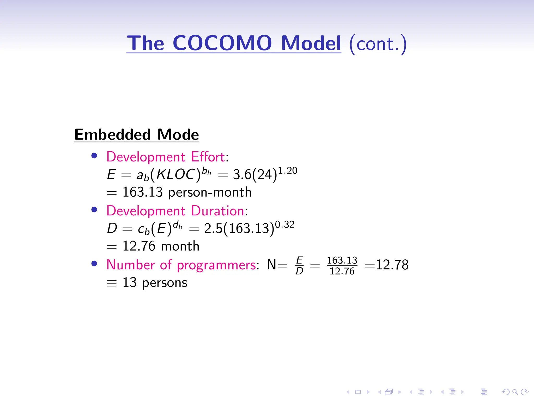
The COCOMO Model(cont.)
Embedded Mode
• Development Effort:
E = ab(KLOC)bb
= 3.6(24)1.20
= 163.13 person-month
• Development Duration:
D = cb(E)db
= 2.5(163.13)0.32
= 12.76 month
• Number of programmers: N= E
D = 163.13
12.76 =12.78
≡ 13 persons
46.
D
r
a
f
t
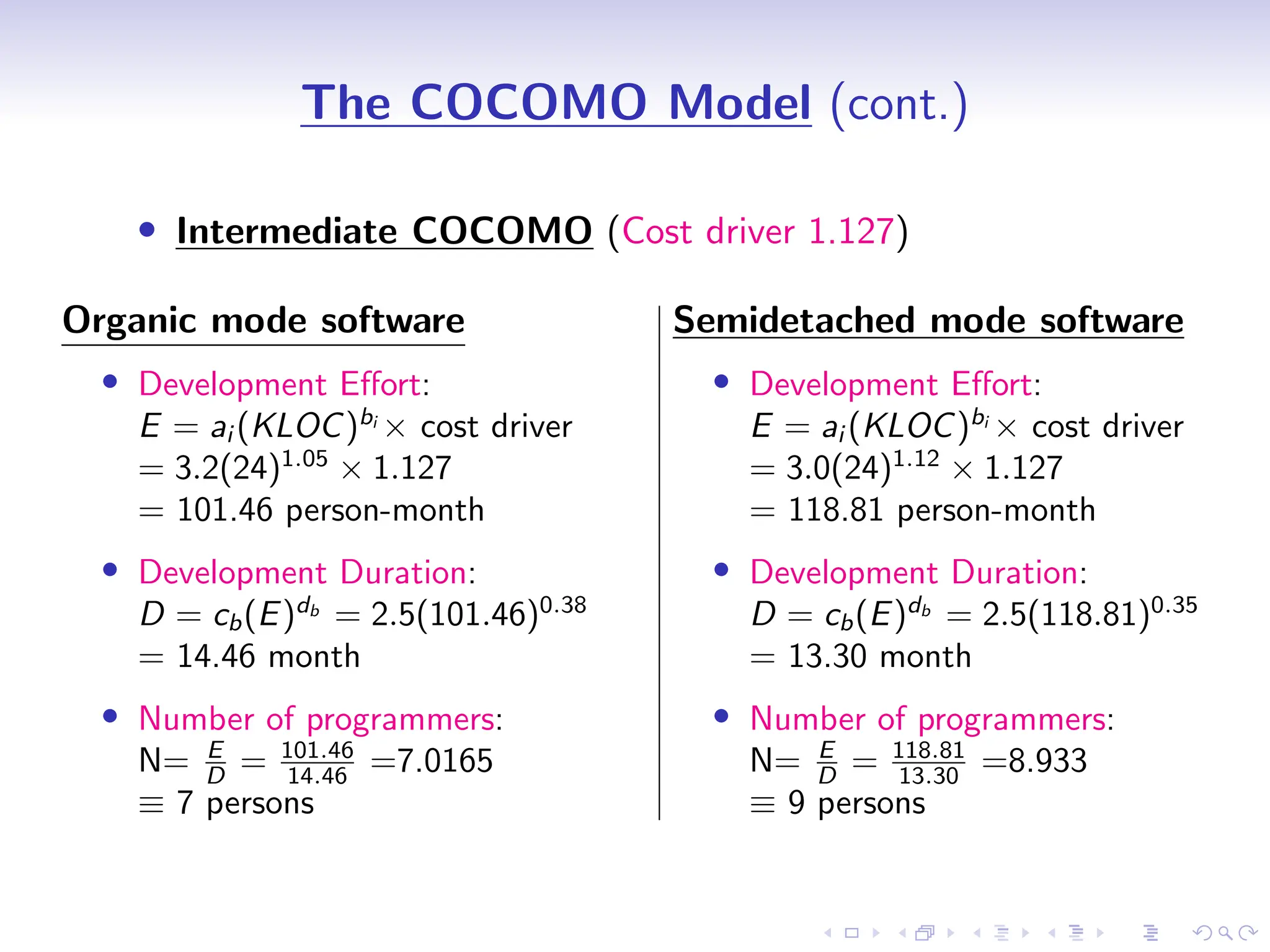
The COCOMO Model(cont.)
• Intermediate COCOMO (Cost driver 1.127)
Organic mode software
• Development Effort:
E = ai (KLOC)bi
× cost driver
= 3.2(24)1.05
× 1.127
= 101.46 person-month
• Development Duration:
D = cb(E)db
= 2.5(101.46)0.38
= 14.46 month
• Number of programmers:
N= E
D = 101.46
14.46 =7.0165
≡ 7 persons
Semidetached mode software
• Development Effort:
E = ai (KLOC)bi
× cost driver
= 3.0(24)1.12
× 1.127
= 118.81 person-month
• Development Duration:
D = cb(E)db
= 2.5(118.81)0.35
= 13.30 month
• Number of programmers:
N= E
D = 118.81
13.30 =8.933
≡ 9 persons
47.
D
r
a
f
t
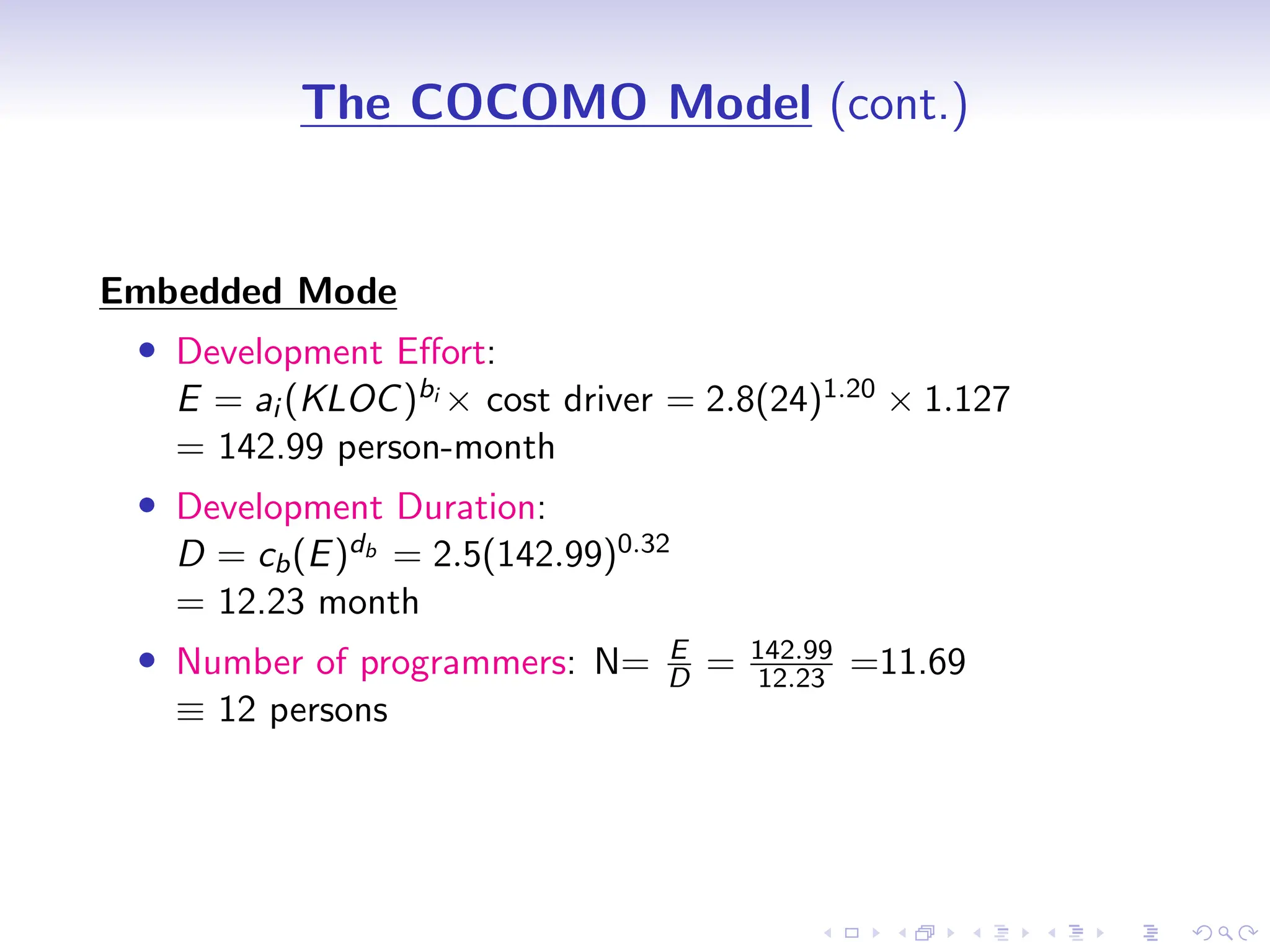
The COCOMO Model(cont.)
Embedded Mode
• Development Effort:
E = ai (KLOC)bi × cost driver = 2.8(24)1.20 × 1.127
= 142.99 person-month
• Development Duration:
D = cb(E)db = 2.5(142.99)0.32
= 12.23 month
• Number of programmers: N= E
D = 142.99
12.23 =11.69
≡ 12 persons
48.
D
r
a
f
t
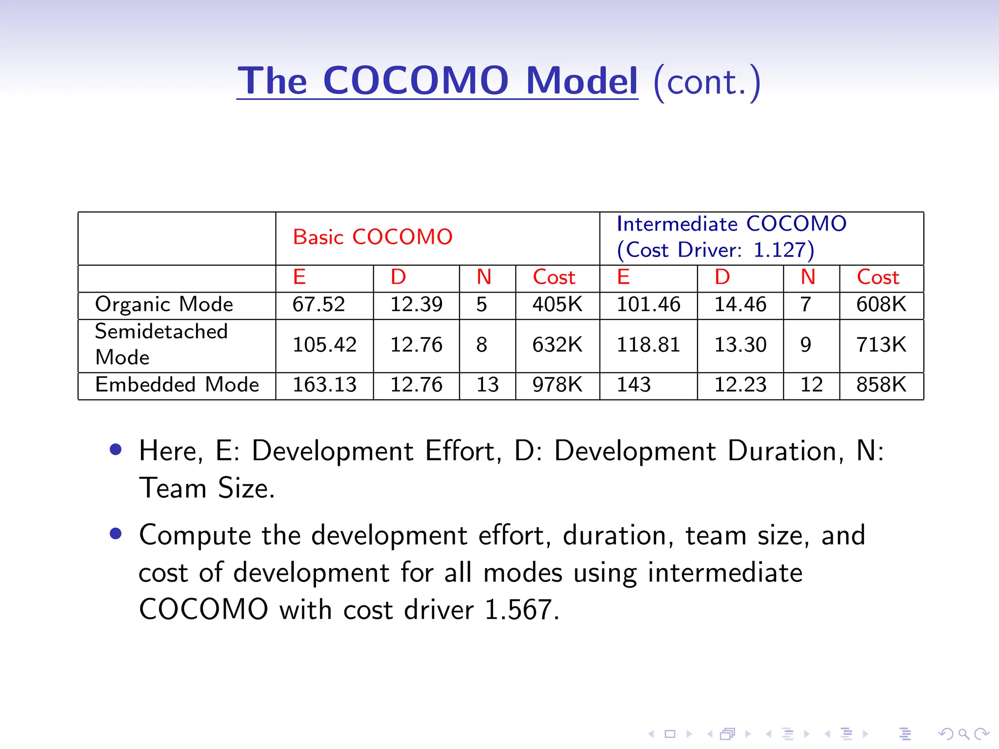
The COCOMO Model(cont.)
Basic COCOMO
Intermediate COCOMO
(Cost Driver: 1.127)
E D N Cost E D N Cost
Organic Mode 67.52 12.39 5 405K 101.46 14.46 7 608K
Semidetached
Mode
105.42 12.76 8 632K 118.81 13.30 9 713K
Embedded Mode 163.13 12.76 13 978K 143 12.23 12 858K
• Here, E: Development Effort, D: Development Duration, N:
Team Size.
• Compute the development effort, duration, team size, and
cost of development for all modes using intermediate
COCOMO with cost driver 1.567.
49.
D
r
a
f
t
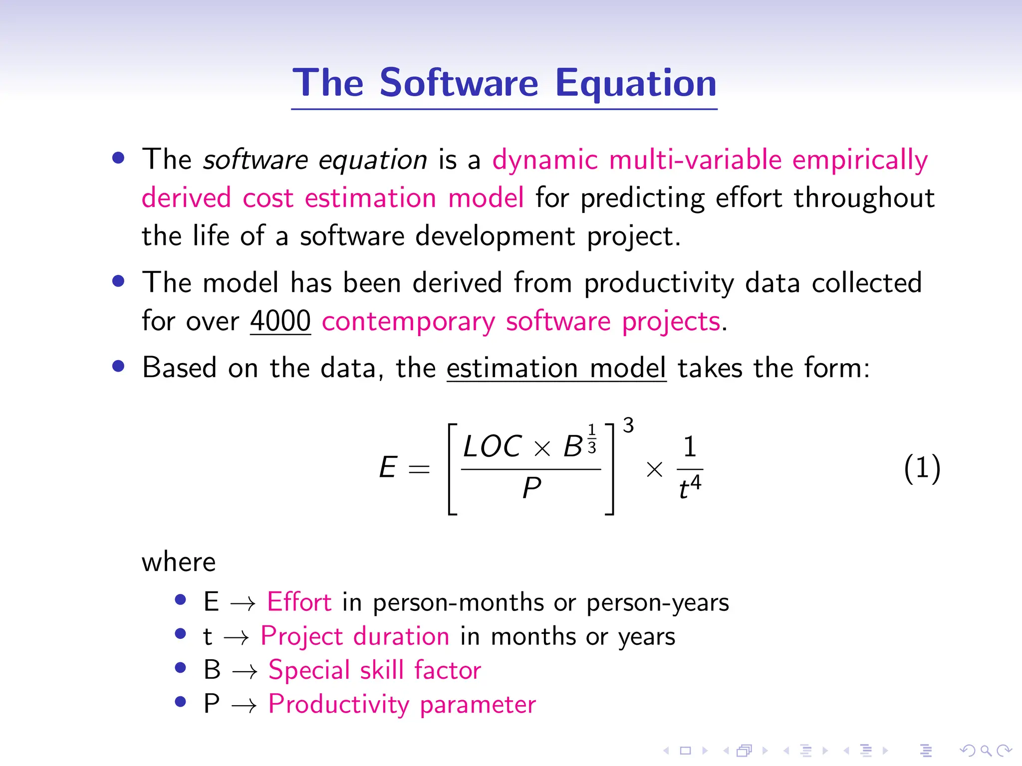
The Software Equation
•The software equation is a dynamic multi-variable empirically
derived cost estimation model for predicting effort throughout
the life of a software development project.
• The model has been derived from productivity data collected
for over 4000 contemporary software projects.
• Based on the data, the estimation model takes the form:
E =
"
LOC × B
1
3
P
#3
×
1
t4
(1)
where
• E → Effort in person-months or person-years
• t → Project duration in months or years
• B → Special skill factor
• P → Productivity parameter
50.
D
r
a
f
t
The Software Equation(cont.)
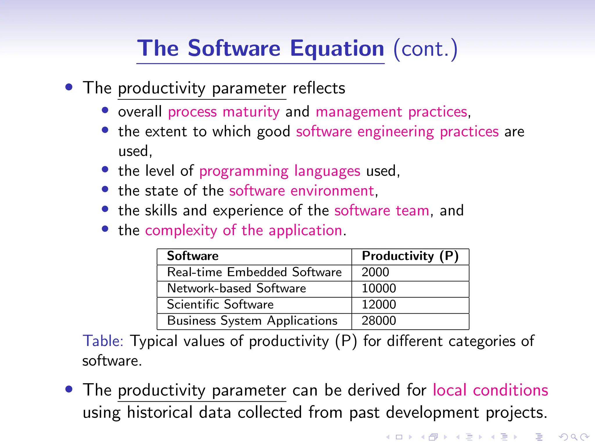
• The productivity parameter reflects
• overall process maturity and management practices,
• the extent to which good software engineering practices are
used,
• the level of programming languages used,
• the state of the software environment,
• the skills and experience of the software team, and
• the complexity of the application.
Software Productivity (P)
Real-time Embedded Software 2000
Network-based Software 10000
Scientific Software 12000
Business System Applications 28000
Table: Typical values of productivity (P) for different categories of
software.
• The productivity parameter can be derived for local conditions
using historical data collected from past development projects.
51.
D
r
a
f
t
The Software Equation(cont.)
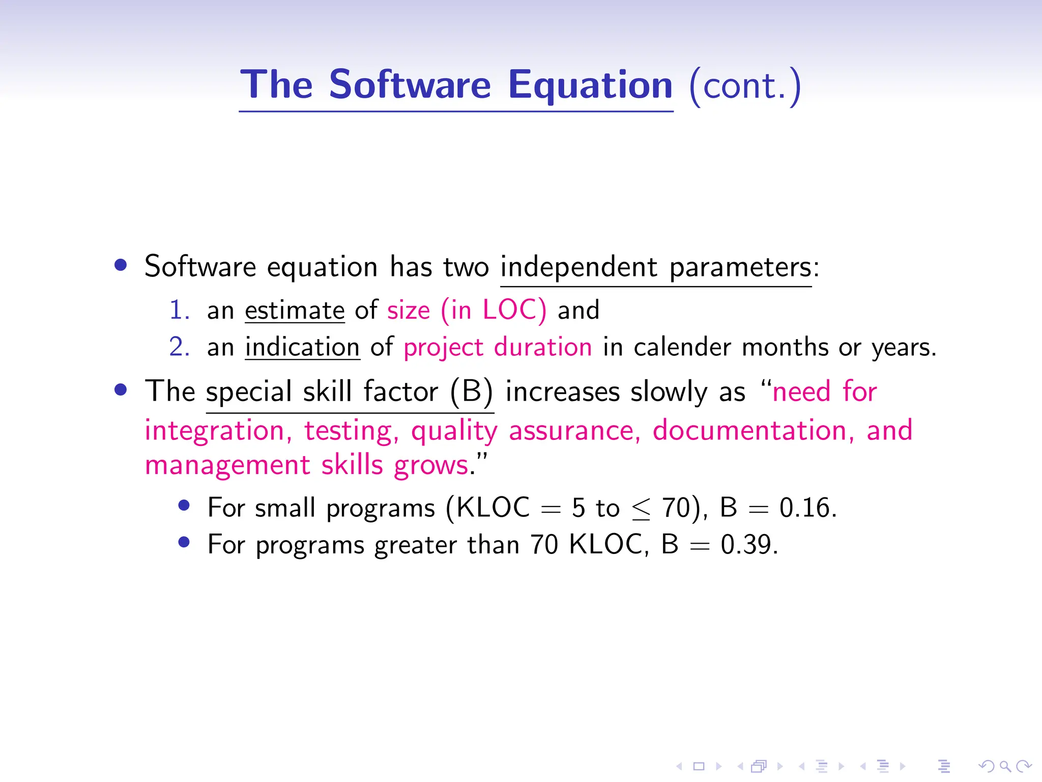
• Software equation has two independent parameters:
1. an estimate of size (in LOC) and
2. an indication of project duration in calender months or years.
• The special skill factor (B) increases slowly as “need for
integration, testing, quality assurance, documentation, and
management skills grows.”
• For small programs (KLOC = 5 to ≤ 70), B = 0.16.
• For programs greater than 70 KLOC, B = 0.39.
52.
D
r
a
f
t
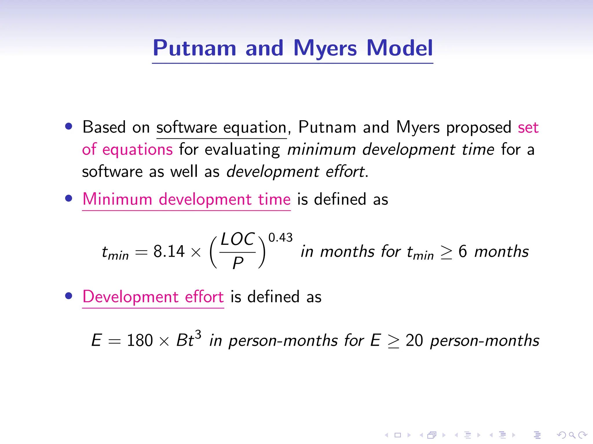
Putnam and MyersModel
• Based on software equation, Putnam and Myers proposed set
of equations for evaluating minimum development time for a
software as well as development effort.
• Minimum development time is defined as
tmin = 8.14 ×
LOC
P
0.43
in months for tmin ≥ 6 months
• Development effort is defined as
E = 180 × Bt3
in person-months for E ≥ 20 person-months
53.
D
r
a
f
t
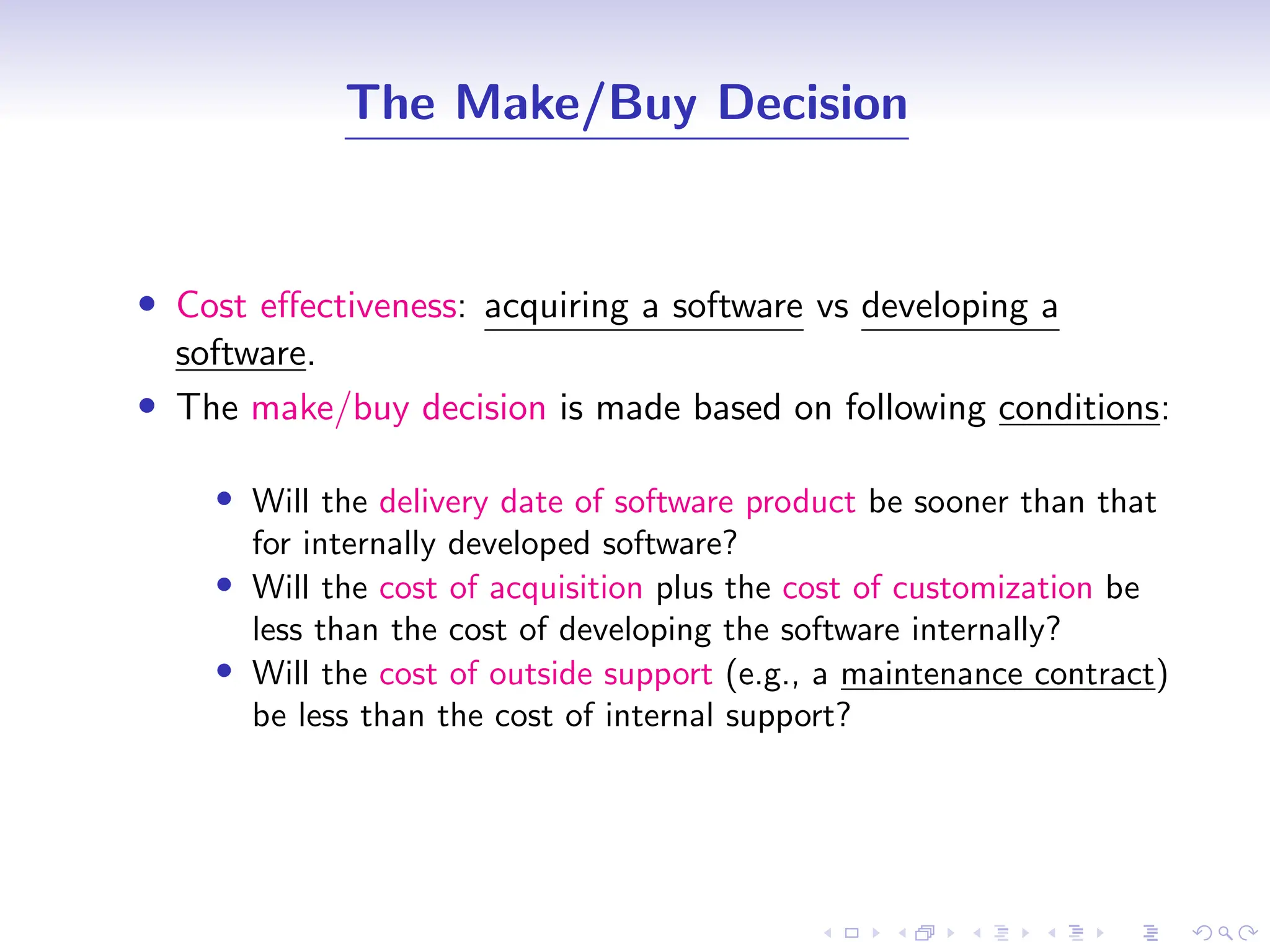
The Make/Buy Decision
•Cost effectiveness: acquiring a software vs developing a
software.
• The make/buy decision is made based on following conditions:
• Will the delivery date of software product be sooner than that
for internally developed software?
• Will the cost of acquisition plus the cost of customization be
less than the cost of developing the software internally?
• Will the cost of outside support (e.g., a maintenance contract)
be less than the cost of internal support?
54.
D
r
a
f
t
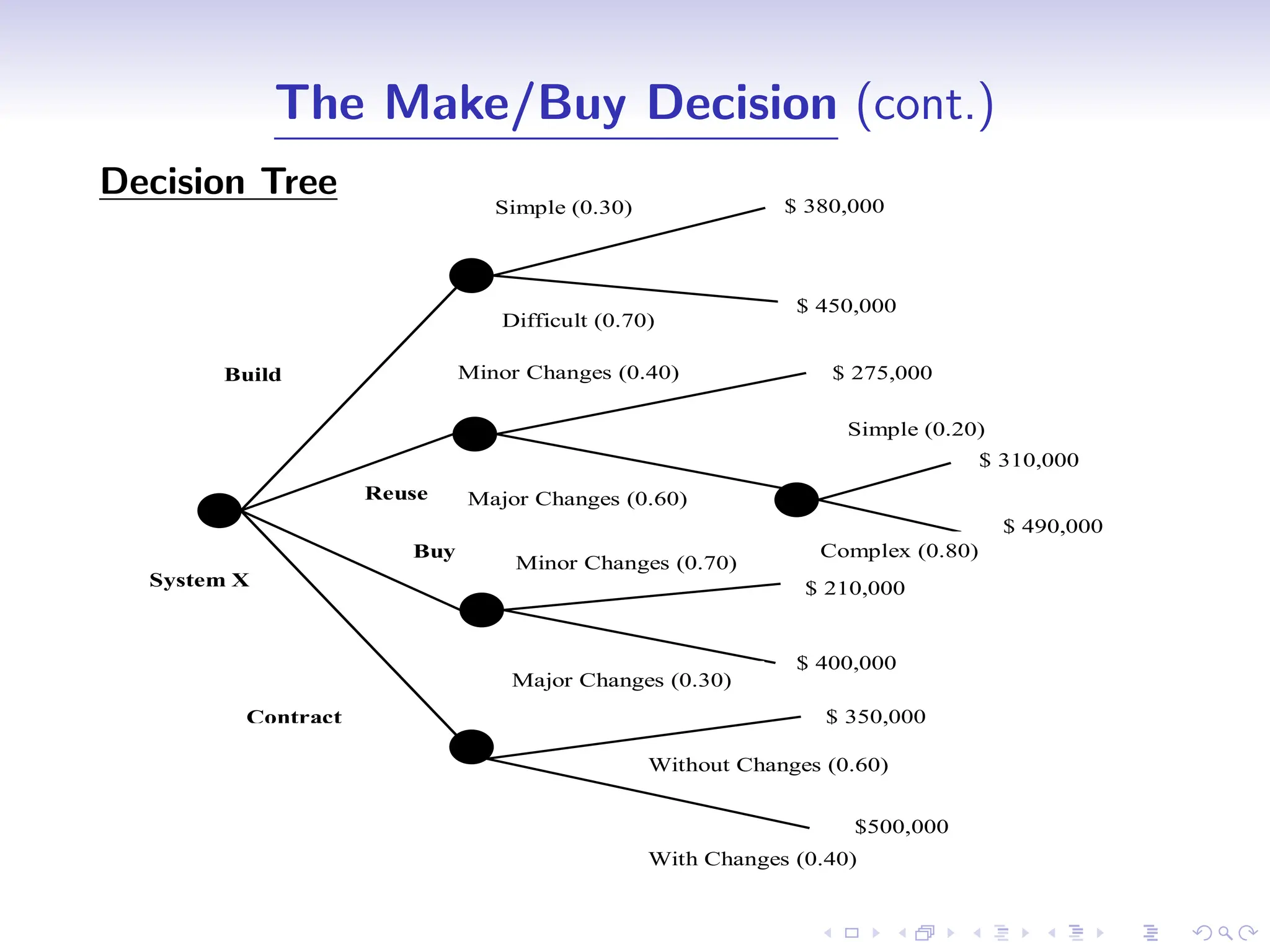
The Make/Buy Decision(cont.)
Decision Tree
Simple (0.30)
Difficult (0.70)
Build
Reuse
Minor Changes (0.40)
Major Changes (0.60)
Buy
Simple (0.20)
Complex (0.80)
Minor Changes (0.70)
Major Changes (0.30)
Contract
Without Changes (0.60)
With Changes (0.40)
$ 380,000
$ 450,000
$ 275,000
$ 310,000
$ 490,000
$ 210,000
$ 400,000
$ 350,000
$500,000
System X
55.
D
r
a
f
t
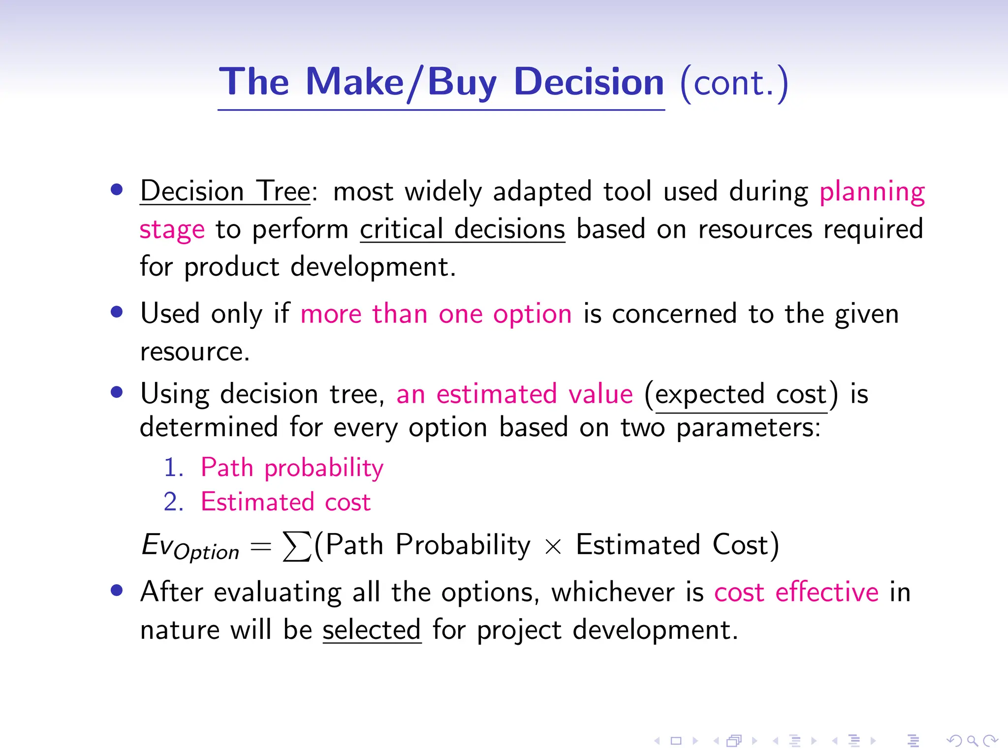
The Make/Buy Decision(cont.)
• Decision Tree: most widely adapted tool used during planning
stage to perform critical decisions based on resources required
for product development.
• Used only if more than one option is concerned to the given
resource.
• Using decision tree, an estimated value (expected cost) is
determined for every option based on two parameters:
1. Path probability
2. Estimated cost
EvOption =
P
(Path Probability × Estimated Cost)
• After evaluating all the options, whichever is cost effective in
nature will be selected for project development.
56.
D
r
a
f
t
The Make/Buy Decision(cont.)
• Expected Costbuild = 0.30($380K) + 0.70($450K) = $429K
• Expected Costreuse =
0.40($275K) + 0.60[0.20($310K) + 0.80($490K)] = $382K
• Expected Costbuy = 0.70($210K) + 0.30($400K) = $267K
• Expected Costcontract =
0.60($350K) + 0.40($500K) = $410K
![D
r
a
f
t
The Make/Buy Decision (cont.)
• Expected Costbuild = 0.30($380K) + 0.70($450K) = $429K
• Expected Costreuse =
0.40($275K) + 0.60[0.20($310K) + 0.80($490K)] = $382K
• Expected Costbuy = 0.70($210K) + 0.30($400K) = $267K
• Expected Costcontract =
0.60($350K) + 0.40($500K) = $410K](https://image.slidesharecdn.com/softwareprojectplanningandestimation-250406160913-8d1d96a7/75/Software-Project-Planning-and-Estimation-pdf-56-2048.jpg)


![Understanding Parkinson’s Disease: Causes, Symptoms, and Treatment [2025]](https://cdn.slidesharecdn.com/ss_thumbnails/understandingparkinson-251208102525-80ba3223-thumbnail.jpg?width=640&height=640&fit=bounds)


