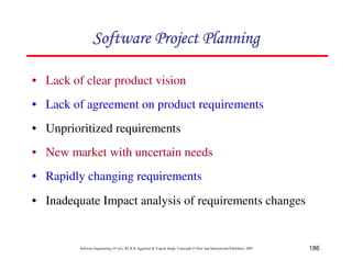
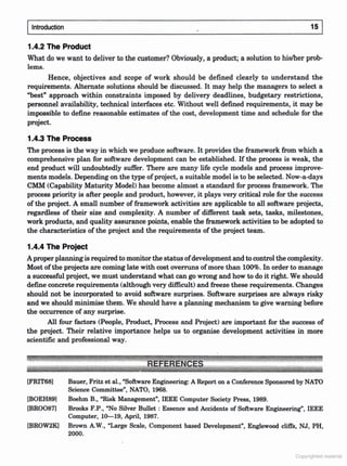
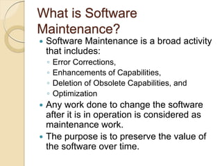
What is Software
Maintenance?
Software Maintenance is a broad activity
that includes:
│ Error Corrections,
│ Enhancements of Capabilities,
│ Deletion of Obsolete Capabilities, and
│ Optimization
Any work done to change the software
after it is in operation is considered as
maintenance work.
The purpose is to preserve the value of
the software over time.
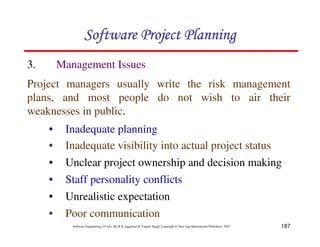
3.
Categories of Maintenance
There are three major categories of
software maintenance:
│ Corrective Maintenance
│ Adaptive Maintenance
│ Perfective Maintenance
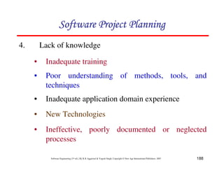
4.
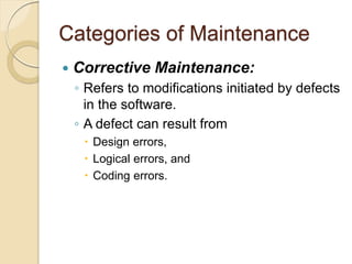
Categories of Maintenance
Corrective Maintenance:
│ Refers to modifications initiated by defects
in the software.
│ A defect can result from
Design errors,
Logical errors, and
Coding errors.
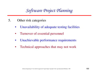
5.
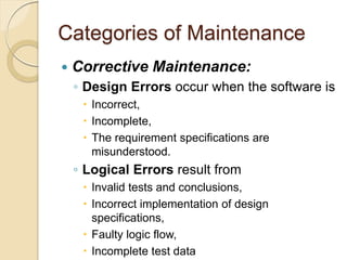
Categories of Maintenance
Corrective Maintenance:
│ Design Errors occur when the software is
Incorrect,
Incomplete,
The requirement specifications are
misunderstood.
│ Logical Errors result from
Invalid tests and conclusions,
Incorrect implementation of design
specifications,
Faulty logic flow,
Incomplete test data
6.
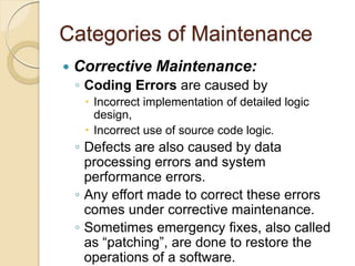
Categories of Maintenance
Corrective Maintenance:
│ Coding Errors are caused by
Incorrect implementation of detailed logic
design,
Incorrect use of source code logic.
│ Defects are also caused by data
processing errors and system
performance errors.
│ Any effort made to correct these errors
comes under corrective maintenance.
│ Sometimes emergency fixes, also called
as “patching”, are done to restore the
operations of a software.
7.
Categories of Maintenance
Adaptive Maintenance:
│ It includes modifying the software to
match changes in the environment.
│ Environment refers to the totality of all
conditions and influences which act upon
the software from outside.
│ For example,
Business rules,
Government policies,
Work patterns,
Software and hardware operating platforms.
8.
Categories of Maintenance
Adaptive Maintenance:
│ This type of maintenance includes any
work that has been started due to moving
the software to a different hardware or
software platform (a new operating
system or a new processor).
9.
Categories of Maintenance
Perfective Maintenance:
│ It means improving processing efficiency
or performance of the software.
│ It also means restructuring the software to
improve changeability.
│ When software becomes useful, the user
may want to extend it beyond the scope
for which it was initially developed.
10.
Categories of Maintenance
Perfective Maintenance:
│ Expansion in requirements then results in
enhancements to the existing system
functionality or efficiency.
│ Thus, Perfective maintenance refers to
enhancements to make the product better,
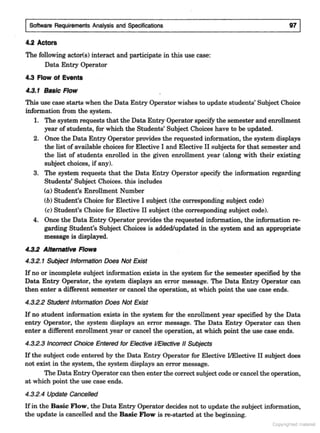
faster, and cleanly structured with more
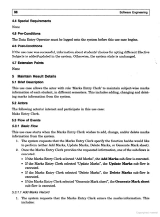
functions and reports.
11.
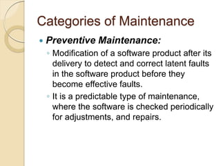
Categories of Maintenance
Preventive Maintenance:
│ Modification of a software product after its
delivery to detect and correct latent faults
in the software product before they
become effective faults.
│ It is a predictable type of maintenance,
where the software is checked periodically
for adjustments, and repairs.
12.
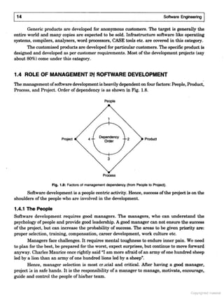
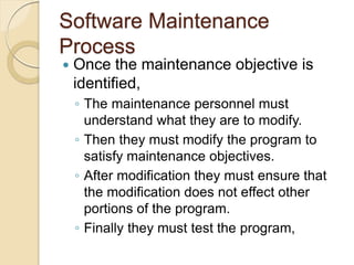
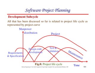
Software Maintenance
Process
Oncethe maintenance objective is
identified,
│ The maintenance personnel must
understand what they are to modify.
│ Then they must modify the program to
satisfy maintenance objectives.
│ After modification they must ensure that
the modification does not effect other
portions of the program.
│ Finally they must test the program,
13.
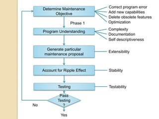
Determine Maintenance
Objective
Program Understanding
Generateparticular
maintenance proposal
Account for Ripple Effect
Testing
Pass
Testing
?
Correct program error
Add new capabilities
Delete obsolete features
Optimization
Phase 1
Complexity
Documentation
Self descriptiveness
Extensibility
Stability
Testability
Yes
No
14.
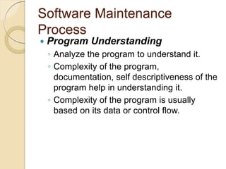
Software Maintenance
Process
ProgramUnderstanding
│ Analyze the program to understand it.
│ Complexity of the program,
documentation, self descriptiveness of the
program help in understanding it.
│ Complexity of the program is usually
based on its data or control flow.
15.
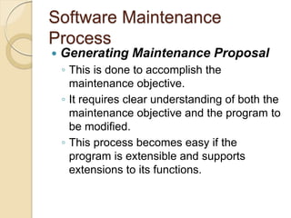
Software Maintenance
Process
GeneratingMaintenance Proposal
│ This is done to accomplish the
maintenance objective.
│ It requires clear understanding of both the
maintenance objective and the program to
be modified.
│ This process becomes easy if the
program is extensible and supports
extensions to its functions.
16.
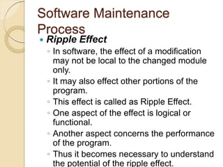
Software Maintenance
Process
RippleEffect
│ In software, the effect of a modification
may not be local to the changed module
only.
│ It may also effect other portions of the
program.
│ This effect is called as Ripple Effect.
│ One aspect of the effect is logical or
functional.
│ Another aspect concerns the performance
of the program.
│ Thus it becomes necessary to understand
the potential of the ripple effect.
17.
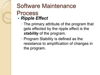
Software Maintenance
Process
RippleEffect
│ The primary attribute of the program that
gets effected by the ripple effect is the
stability of the program.
│ Program Stability is defined as the
resistance to amplification of changes in
the program.
18.
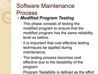
Software Maintenance
Process
ModifiedProgram Testing
│ This phase consists of testing the
modified program to ensure that the
modified program has the same reliability
level as before.
│ It is important that cost effective testing
techniques be applied during
maintenance.
│ The testing process becomes cost
effective due to the testability of the
program.
│ Program Testability is defined as the effort
19.
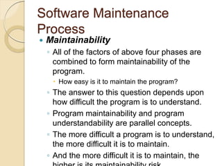
Software Maintenance
Process
Maintainability
│All of the factors of above four phases are
combined to form maintainability of the
program.
How easy is it to maintain the program?
│ The answer to this question depends upon
how difficult the program is to understand.
│ Program maintainability and program
understandability are parallel concepts.
│ The more difficult a program is to understand,
the more difficult it is to maintain.
│ And the more difficult it is to maintain, the
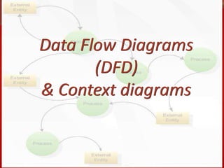
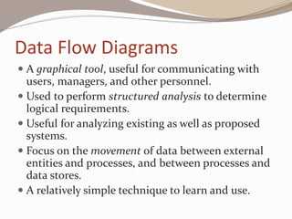
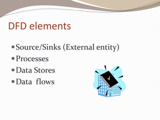
Data Flow Diagrams
A graphical tool, useful for communicating with
users, managers, and other personnel.
Used to perform structured analysis to determine
logical requirements.
Useful for analyzing existing as well as proposed
systems.
Focus on the movement of data between external
entities and processes, and between processes and
data stores.
A relatively simple technique to learn and use.
264.
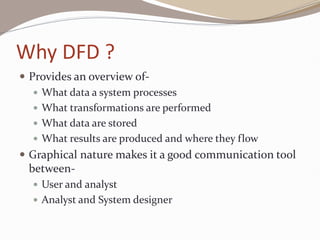
Why DFD ?
Provides an overview of-
What data a system processes
What transformations are performed
What data are stored
What results are produced and where they flow
Graphical nature makes it a good communication tool
between-
User and analyst
Analyst and System designer
5
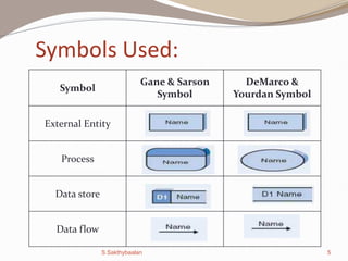
Symbols Used:
Symbol
Gane Sarson
Symbol
DeMarco
Yourdan Symbol
External Entity
Process
Data store
Data flow
S.Sakthybaalan
267.
6
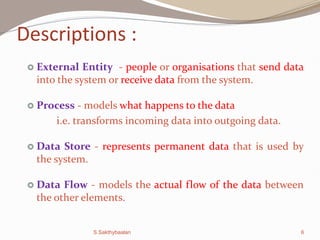
Descriptions :
ExternalEntity - people or organisations that send data
into the system or receive data from the system.
Process - models what happens to the data
i.e. transforms incoming data into outgoing data.
Data Store - represents permanent data that is used by
the system.
Data Flow - models the actual flow of the data between
the other elements.
S.Sakthybaalan
268.
7
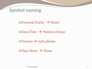
External Entity Noun
Data Flow Names of data
Process verb phrase
Data Store Noun
Symbol naming
S.Sakthybaalan
269.
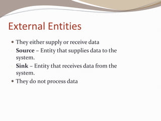
External Entities
Theyeither supply or receive data
• Source Entity that supplies data to the
system.
• Sink Entity that receives data from the
system.
They do not process data
270.
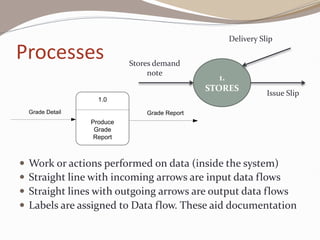
Processes
Work oractions performed on data (inside the system)
Straight line with incoming arrows are input data flows
Straight lines with outgoing arrows are output data flows
Labels are assigned to Data flow. These aid documentation
1.
STORES
Stores demand
note
Delivery Slip
Issue Slip
1.0
Produce
Grade
Report
Grade Detail Grade Report
271.
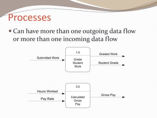
Processes
Can havemore than one outgoing data flow
or more than one incoming data flow
1.0
Grade
Student
Work
Submitted Work
Graded Work
Student Grade
3.0
Calculated
Gross
Pay
Hours Worked
Pay Rate
Gross Pay
272.
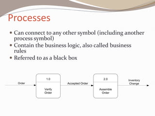
Processes
Can connectto any other symbol (including another
process symbol)
Contain the business logic, also called business
rules
Referred to as a black box
1.0
Verify
Order
2.0
Assemble
Order
Order Accepted Order
Inventory
Change
273.
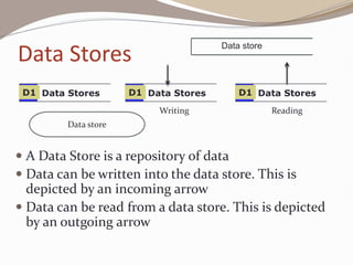
Data Stores
AData Store is a repository of data
Data can be written into the data store. This is
depicted by an incoming arrow
Data can be read from a data store. This is depicted
by an outgoing arrow
Data Stores
D1 Data Stores
D1 Data Stores
D1
Writing Reading
Data store
Data store
274.
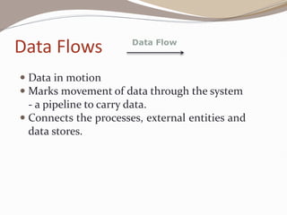
Data Flows
Datain motion
Marks movement of data through the system
- a pipeline to carry data.
Connects the processes, external entities and
data stores.
Data Flow
275.
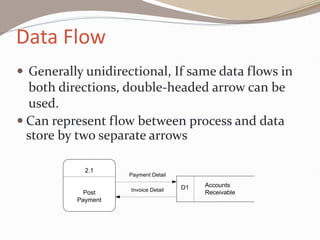
Data Flow
Generallyunidirectional, If same data flows in
both directions, double-headed arrow can be
used.
Can represent flow between process and data
store by two separate arrows
2.1
Post
Payment
Accounts
Receivable
D1
Payment Detail
Invoice Detail
276.
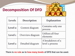
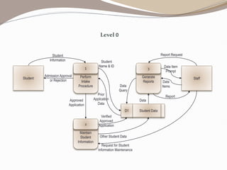
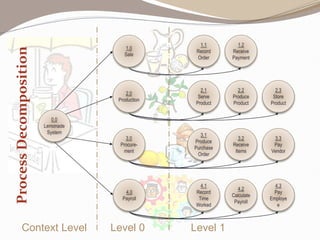
Decomposition Of DFD
LevelsDescription Explanation
Level 0 Context diagram
Contains only one
process
Level 1 Overview diagram
Utilizes all four
elements
Level 2 Detailed diagram
A breakdown of a
level 2 process
There is no rule as to how many levels of DFD that can be used.
277.
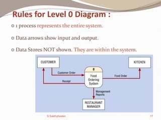
17
Rules for Level0 Diagram :
1 process represents the entire system.
Data arrows show input and output.
Data Stores NOT shown. They are within the system.
S.Sakthybaalan
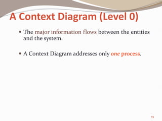
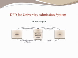
A Context Diagram(Level 0)
The major information flows between the entities
and the system.
A Context Diagram addresses only one process.
19
280.
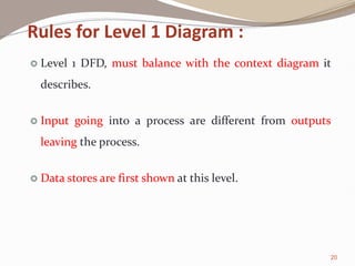
20
Rules for Level1 Diagram :
Level 1 DFD, must balance with the context diagram it
describes.
Input going into a process are different from outputs
leaving the process.
Data stores are first shown at this level.
281.
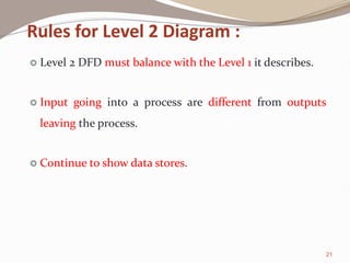
21
Rules for Level2 Diagram :
Level 2 DFD must balance with the Level 1 it describes.
Input going into a process are different from outputs
leaving the process.
Continue to show data stores.
282.
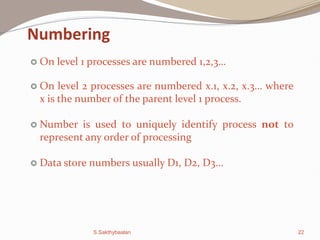
22
Numbering
On level1 processes are numbered 1,2,3
On level 2 processes are numbered x.1, x.2, x.3 where
x is the number of the parent level 1 process.
Number is used to uniquely identify process not to
represent any order of processing
Data store numbers usually D1, D2, D3...
S.Sakthybaalan
283.
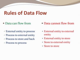
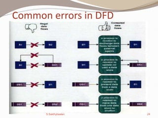
Rules of DataFlow
Data can flow from
External entity to process
Process to external entity
Process to store and back
Process to process
Data cannot flow from
External entity to external
entity
External entity to store
Store to external entity
Store to store
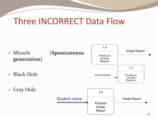
25
Miracle (Spontaneous
generation)
Black Hole
Gray Hole
1.0
Produce
Grade
Report
Grade Report
1.0
Produce
Grade
Report
Grade Detail
1.0
Produce
Grade
Report
Grade Report
Student name
Three INCORRECT Data Flow
286.
Good Style inDrawing DFD
Use meaningful names for data flows, processes and
data stores.
Use top down development starting from context
diagram and successively levelling DFD
Only previously stored data can be read
A process can only transfer input to output. It cannot
create new data
Data stores cannot create new data
287.
Creating DFDs
Createa preliminary Context Diagram.
Identify Use Cases, i.e. the ways in which users most
commonly use the system.
Create DFD fragments for each use case.
Create a Level 0 diagram from fragments.
Decompose to Level
Validate DFDs with users.
288.
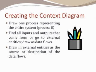
Creating the ContextDiagram
Draw one process representing
the entire system (process 0)
Find all inputs and outputs that
come from or go to external
entities; draw as data flows.
Draw in external entities as the
source or destination of the
data flows.
289.
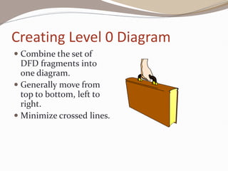
Creating Level 0Diagram
Combine the set of
DFD fragments into
one diagram.
Generally move from
top to bottom, left to
right.
Minimize crossed lines.
290.
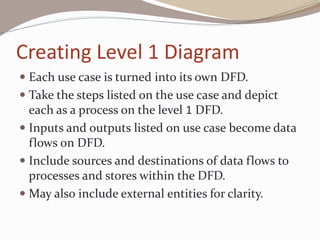
Creating Level 1Diagram
Each use case is turned into its own DFD.
Take the steps listed on the use case and depict
each as a process on the level 1 DFD.
Inputs and outputs listed on use case become data
flows on DFD.
Include sources and destinations of data flows to
processes and stores within the DFD.
May also include external entities for clarity.
291.
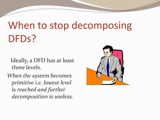
When to stopdecomposing
DFDs?
Ideally, a DFD has at least
three levels.
When the system becomes
primitive i.e. lowest level
is reached and further
decomposition is useless.
292.
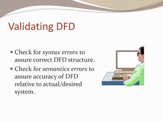
Validating DFD
Checkfor syntax errors to
assure correct DFD structure.
Check for semantics errors to
assure accuracy of DFD
relative to actual/desired
system.
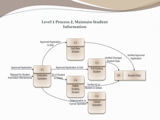
Add New
Student
2.2
Edit Existing
Student
2.3
Delete
Existing
Student
2.4
StudentData
D1
Cancel
Operation
2.5
Approved Application to Edit
ID of Student
to Delete
Determination to
Cancel Operation
Determine
Operation
2.1
Approved Application
Request for Student
Information Maintenance
Approved Application
to Add
Verified Approved
Application
Verified Changed
Student Data
Verified ID of
Student to Delete
Level 1 Process 2, Maintain Student
Information
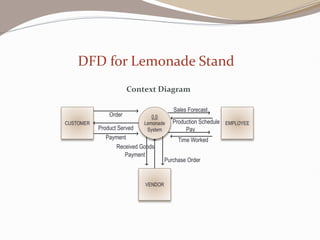
297.
Context Diagram
DFD forLemonade Stand
0.0
Lemonade
System
EMPLOYEE
CUSTOMER
Pay
Payment
Order
VENDOR
Payment
Purchase Order
Production Schedule
Received Goods
Time Worked
Sales Forecast
Product Served
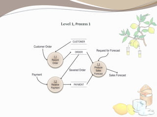
Level 1, Process1
1.3
Produce
Sales
Forecast
Sales Forecast
Payment
1.1
Record
Order
Customer Order
ORDER
1.2
Receive
Payment
PAYMENT
Severed Order
Request for Forecast
CUSTOMER
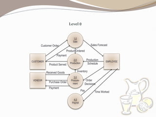
300.
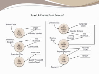
Level 1, Process2 and Process 3
2.1
Serve
Product
Product Order
ORDER
2.2
Produce
Product
INVENTORTY
Quantity Severed
Production
Schedule
RAW
MATERIALS
2.3
Store
Product
Quantity Produced
Location Stored
Quantity Used
Production Data
3.1
Produce
Purchase
Order
Order Decision
PURCHASE
ORDER
3.2
Receive
Items
Received
Goods
RAW
MATERIALS
3.3
Pay
Vendor
Quantity
Received
Quantity On-Hand
RECEIVED
ITEMS
VENDOR
Payment Approval
Payment
301.
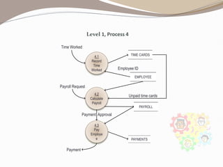
Level 1, Process4
Time Worked
4.1
Record
Time
Worked
TIME CARDS
4.2
Calculate
Payroll
Payroll Request
EMPLOYEE
4.3
Pay
Employe
e
Employee ID
PAYROLL
PAYMENTS
Payment Approval
Payment
Unpaid time cards
Logical and PhysicalDFD
DFDs considered so far are called logical DFDs
A physical DFD is similar to a document flow diagram
It specifies who does the operations specified by the
logical DFD
Physical DFD may depict physical movements of the
goods
Physical DFDs can be drawn during fact gathering
phase of a life cycle
304.
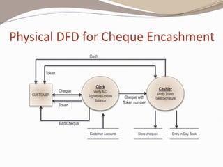
Physical DFD forCheque Encashment
Cash
Clerk
Verify A/C
Signature Update
Balance
Bad Cheque
Store cheques
Customer Accounts
Cheque
Cheque with
Token number
Cashier
Verify Token
Take Signature
Entry in Day Book
CUSTOMER
Token
Token
305.
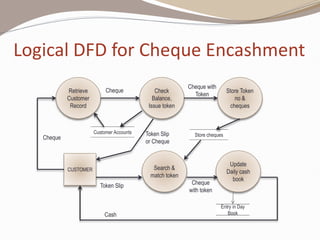
Logical DFD forCheque Encashment
Cash
Retrieve
Customer
Record
Cheque
with token
Store cheques
Customer Accounts
Cheque
Cheque with
Token
Entry in Day
Book
CUSTOMER
Token Slip
Cheque Check
Balance,
Issue token
Store Token
no
cheques
Search
match token
Update
Daily cash
book
Token Slip
or Cheque
In aDFD external entities are represented by a
a. Rectangle
b. Ellipse
c. Diamond shaped box
d. Circle
External Entities may be a
a. Source of input data only
b. Source of input data or destination of results
c. Destination of results only
d. Repository of data
A data store in a DFD represents
a. A sequential file
b. A disk store
c. A repository of data
d. A random access memory
308.
By anexternal entity we mean a
a. Unit outside the system being designed which can be controlled by an analyst
b. Unit outside the system whose behaviour is independent of the system being
designed
c. A unit external to the system being designed
d. A unit which is not part of DFD
A data flow can
a. Only enter a data store
b. Only leave a data store
c. Enter or leave a data store
d. Either enter or leave a data store but not both
A circle in a DFD represents
a. A data store
b. A an external entity
c. A process
d. An input unit
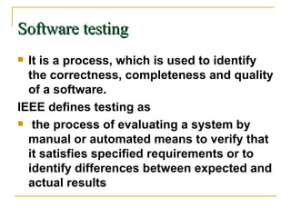
Why Testing isnecessary
Testing Techniques
Test Planning
Test Specification and Execution
Psychology of Testing
Defect Management
Test Automation
313.
What is Testing?
Testing is a process used to identify the correctness,
completeness and quality of developed computer
software. Testing, apart from finding errors, is also used
to test performance, safety, fault-tolerance or security.
Software testing is a broad term that covers a variety of
processes designed to ensure that software
applications function as intended, are able to handle
the volume required, and integrate correctly with other
software applications.
314.
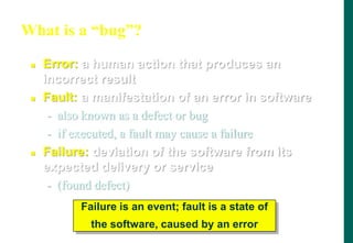
What is a“bug”?
Error: a human action that produces an
incorrect result
Fault: a manifestation of an error in software
- also known as a defect or bug
- if executed, a fault may cause a failure
Failure: deviation of the software from its
expected delivery or service
- (found defect)
Failure is an event; fault is a state of
the software, caused by an error
315.
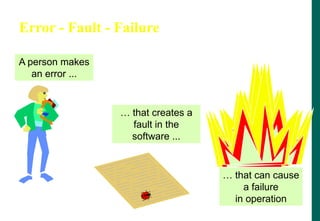
Error - Fault- Failure
A person makes
an error ...
… that creates a
fault in the
software ...
… that can cause
a failure
in operation
316.
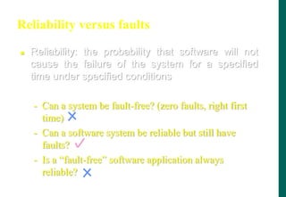
Reliability versus faults
Reliability: the probability that software will not
cause the failure of the system for a specified
time under specified conditions
- Can a system be fault-free? (zero faults, right first
time)
- Can a software system be reliable but still have
faults?
- Is a “fault-free” software application always
reliable?
317.
Reliability versus faults
Reliability: the probability that software will not
cause the failure of the system for a specified
time under specified conditions
- Can a system be fault-free? (zero faults, right first
time)
- Can a software system be reliable but still have
faults?
- Is a “fault-free” software application always
reliable?
318.
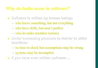
Why do faultsoccur in software?
Software is written by human beings
- who know something, but not everything
- who have skills, but aren‟t perfect
- who do make mistakes (errors)
Under increasing pressure to deliver to strict
deadlines
- no time to check but assumptions may be wrong
- systems may be incomplete
If you have ever written software ...
319.
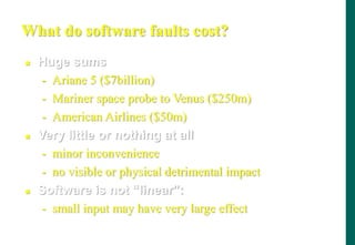
What do softwarefaults cost?
Huge sums
- Ariane 5 ($7billion)
- Mariner space probe to Venus ($250m)
- American Airlines ($50m)
Very little or nothing at all
- minor inconvenience
- no visible or physical detrimental impact
Software is not “linear”:
- small input may have very large effect
320.
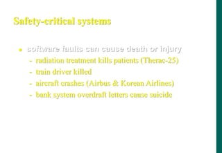
Safety-critical systems
softwarefaults can cause death or injury
- radiation treatment kills patients (Therac-25)
- train driver killed
- aircraft crashes (Airbus Korean Airlines)
- bank system overdraft letters cause suicide
321.
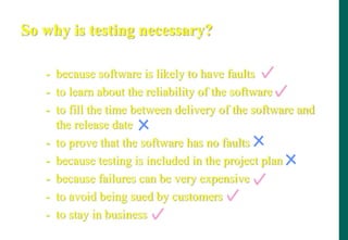
So why istesting necessary?
- because software is likely to have faults
- to learn about the reliability of the software
- to fill the time between delivery of the software and
the release date
- to prove that the software has no faults
- because testing is included in the project plan
- because failures can be very expensive
- to avoid being sued by customers
- to stay in business
322.
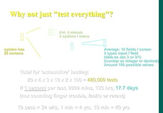
Why not justtest everything?
system has
20 screens
Average: 10 fields / screen
2 types input / field
(date as Jan 3 or 3/1)
(number as integer or decimal)
Around 100 possible values
Total for 'exhaustive' testing:
20 x 4 x 3 x 10 x 2 x 100 = 480,000 tests
If 1 second per test, 8000 mins, 133 hrs, 17.7 days
(not counting finger trouble, faults or retest)
Avr. 4 menus
3 options / menu
10 secs = 34 wks, 1 min = 4 yrs, 10 min = 40 yrs
323.
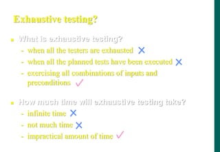
Exhaustive testing?
Whatis exhaustive testing?
- when all the testers are exhausted
- when all the planned tests have been executed
- exercising all combinations of inputs and
preconditions
How much time will exhaustive testing take?
- infinite time
- not much time
- impractical amount of time
324.
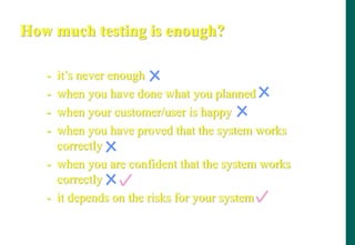
How much testingis enough?
- it‟s never enough
- when you have done what you planned
- when your customer/user is happy
- when you have proved that the system works
correctly
- when you are confident that the system works
correctly
- it depends on the risks for your system
325.
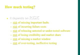
How much testing?
It depends on RISK
- risk of missing important faults
- risk of incurring failure costs
- risk of releasing untested or under-tested software
- risk of losing credibility and market share
- risk of missing a market window
- risk of over-testing, ineffective testing
326.
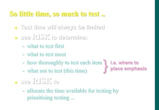
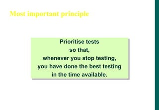
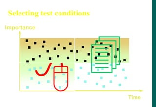
- what notto test (this time)
use RISK to
- allocate the time available for testing by
prioritising testing ...
So little time, so much to test ..
Test time will always be limited
use RISK to determine:
- what to test first
- what to test most
- how thoroughly to test each item
} i.e. where to
place emphasis
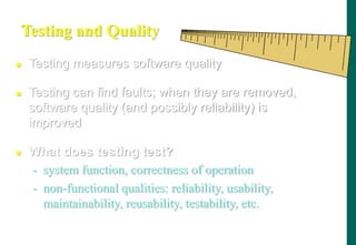
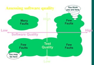
Testing and Quality
Testing measures software quality
Testing can find faults; when they are removed,
software quality (and possibly reliability) is
improved
What does testing test?
- system function, correctness of operation
- non-functional qualities: reliability, usability,
maintainability, reusability, testability, etc.
329.
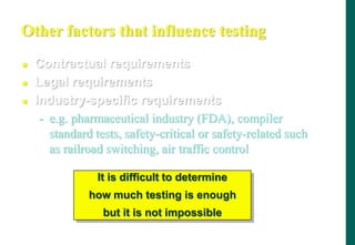
Other factors thatinfluence testing
Contractual requirements
Legal requirements
Industry-specific requirements
- e.g. pharmaceutical industry (FDA), compiler
standard tests, safety-critical or safety-related such
as railroad switching, air traffic control
It is difficult to determine
how much testing is enough
but it is not impossible
Find allthe missing information
• Who
• What
• Where
• When
• Why
• How
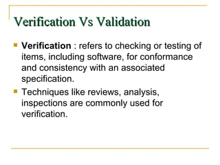
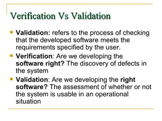
Verification “What to Look For?”
333.
Simply givinga document to a colleague
and asking them to look at it closely which
will identify defects we might never find
on our own.
Peer Review
334.
Informal meetings, whereparticipants come to the
meeting and the author gives the presentation.
Objective:
- To detect defects and become familiar with the material
Elements:
- A planned meeting where only the presenter must
prepare
- A team of 2-7 people, led by the author
- Author usually the presenter.
Inputs:
- Element under examination, objectives for the
walkthroughs applicable standards.
Output:
- Defect report
Walkthrough
335.
Formal meeting, characterizedby individual preparation by all
participants prior to the meeting.
Objectives:
- To obtain defects and collect data.
- To communicate important work product information .
Elements:
- A planned, structured meeting requiring individual
preparation by all participants.
- A team of people, led by an impartial moderator who assure
that rules are being followed and review is effective.
- Presenter is “reader” other than the author.
- Other participants are inspectors who review,
- Recorder to record defects identified in work product
Inspection
336.
An importanttool specially in formal meetings
like inspections
They provide maximum leverage on verification
There are generic checklists that can be applied
at a high level and maintained for each type of
inspection
There are checklists for requirements, functional
design specifications, internal design
specifications, for code
Checklists : the verification tool
337.
Two main strategiesfor validating software
- White Box testing
- Black Box testing
Validation Strategies
338.
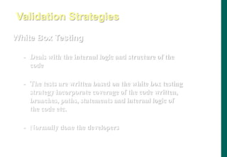
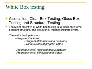
White Box Testing
-Deals with the internal logic and structure of the
code
- The tests are written based on the white box testing
strategy incorporate coverage of the code written,
branches, paths, statements and internal logic of
the code etc.
- Normally done the developers
Validation Strategies
339.
White Box Testingcan be done by:
- Data Coverage
- Code Coverage
White Box testing
340.
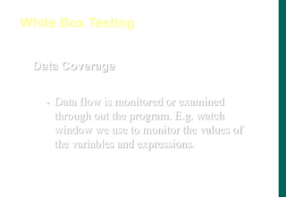
Data Coverage
- Dataflow is monitored or examined
through out the program. E.g. watch
window we use to monitor the values of
the variables and expressions.
White Box Testing
341.
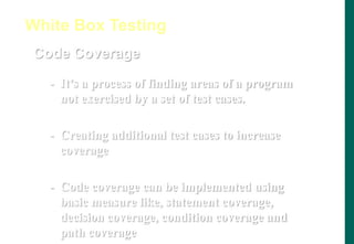
Code Coverage
- It’sa process of finding areas of a program
not exercised by a set of test cases.
- Creating additional test cases to increase
coverage
- Code coverage can be implemented using
basic measure like, statement coverage,
decision coverage, condition coverage and
path coverage
White Box Testing
342.
Black Box Testing
-Does not need any knowledge of internal design or
code
- Its totally based on the testing for the requirements
and functionality of the work product/software
application.
- Tester is needed to be thorough with the
requirement specifications of the system and as a
user, should know how the system should behave in
response to the particular action.
Validation Strategies
343.
Commonly used BlackBox methods :
- Equivalence partitioning
- Boundary-value analysis
- Error guessing
Black Box testing Methods
344.
An equivalenceclass is a subset of data that is
representative of a larger class.
Equivalence partitioning is a technique for testing
equivalence classes rather than undertaking
exhaustive testing of each value of the larger
class.
Equivalence Partitioning
345.
If we expectthe same result from two tests, you consider
them equivalent. A group of tests from an equivalence
class if,
- They all test the same thing
- If one test catches a bug, the others probably will too
- If one test doesn’t catch a bug, the others probably won’t either
Equivalence Partitioning
346.
For example, aprogram which edits credit limits
within a given range ($10,000-$15,000) would
have three equivalence classes:
- Less than $10,000 (invalid)
- Between $10,000 and $15,000 (valid)
- Greater than $15,000 (invalid)
Equivalence Partitioning
347.
Partitioning systeminputs and outputs into
„equivalence sets‟
- If input is a 5-digit integer between 10,000 and 99,999
equivalence partitions are 10,000, 10,000-99,999 and
99,999
The aim is to minimize the number of test cases
required to cover these input conditions
Equivalence Partitioning
348.
Equivalence classes maybe defined according to the
following guidelines:
- If an input condition specifies a range, one valid and two
invalid equivalence classes are defined.
- If an input condition requires a specific value, then one valid
and two invalid equivalence classes are defined.
- If an input condition is Boolean, then one valid and one
invalid equivalence class are defined.
Equivalence Partitioning
349.
Divide theinput domain into classes of data for which test
cases can be generated.
Attempting to uncover classes of errors.
Based on equivalence classes for input conditions.
An equivalence class represents a set of valid or invalid
states
An input condition is either a specific numeric value, range
of values, a set of related values, or a Boolean condition.
Equivalence classes can be defined by:
If an input condition specifies a range or a specific value,
one valid and two invalid equivalence classes defined.
If an input condition specifies a Boolean or a member of a
set, one valid and one invalid equivalence classes defined.
Test cases for each input domain data item developed and
executed.
Equivalence Partitioning Summary
350.
“Bugs lurkin corners and congregate at boundaries…”
Boris Beizer
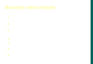
Boundary value analysis
351.
A techniquethat consists of developing test cases and data
that focus on the input and output boundaries of a given
function.
In same credit limit example, boundary analysis would test:
- Low boundary plus or minus one ($9,999 and $10,001)
- On the boundary ($10,000 and $15,000)
- Upper boundary plus or minus one ($14,999 and $15,001)
Boundary value analysis
352.
Large numberof errors tend to occur at boundaries of the input
domain
BVA leads to selection of test cases that exercise boundary
values
BVA complements equivalence partitioning. Rather than select
any element in an equivalence class, select those at the ''edge' of
the class
Examples:
For a range of values bounded by a and b, test (a-1), a, (a+1), (b-1),
b, (b+1)
If input conditions specify a number of values n, test with (n-1), n
and (n+1) input values
Apply 1 and 2 to output conditions (e.g., generate table of
minimum and maximum size)
Boundary value analysis
353.
Example: Loan application
CustomerName
Account number
Loan amount requested
Term of loan
Monthly repayment
Term:
Repayment:
Interest rate:
Total paid back:
6 digits, 1st
non-zero
£500 to £9000
1 to 30 years
Minimum £10
2-64 chars.
354.
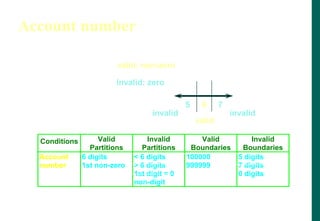
Account number
5 67
invalid
valid
invalid
Number of digits:
First character:
invalid: zero
valid: non-zero
Conditions Valid
Partitions
Invalid
Partitions
Valid
Boundaries
Invalid
Boundaries
Account
number
6 digits
1st non-zero
6 digits
6 digits
1st digit = 0
non-digit
100000
999999
5 digits
7 digits
0 digits
355.
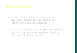
Based onthe theory that test cases can be
developed based upon the intuition and
experience of the Test Engineer
For example, in an example where one of the
inputs is the date, a test engineer might try
February 29,2000 or 9/9/99
Error Guessing
356.
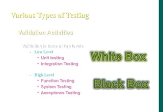
Various Types ofTesting
Validation is done at two levels
- Low Level
• Unit testing
• Integration Testing
- High Level
• Function Testing
• System Testing
• Acceptance Testing
Validation Activities
357.
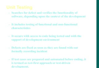
- Searches fordefect and verifies the functionality of
software, depending upon the context of the development
- It includes testing of functional and non-functional
characteristics
- It occurs with access to code being tested and with the
support of development environment
- Defects are fixed as soon as they are found with out
formally recording incident
- If test cases are prepared and automated before coding, it
is termed as test-first approach or test-driven
development.
Unit Testing
358.
Integration Testing
Integrationtesting tests interface between
components, interaction to different parts of system.
Greater the scope of Integration, more it becomes to
isolate failures to specific component or system, which
may leads to increased risk.
Integration testing should normally be integral rather
than big bang, in order to reduce the risk of late defect
discovery
Non functional characteristics (e.g. performance) may
be included in Integration Testing
359.
Functional Testing
Itis used to detect discrepancies between a program‟s
functional specification and the actual behavior of an
application.
The goal of function testing is to verify whether your
product meets the intended functional specifications
laid out the development documentation.
When a discrepancy is detected, either the program or
the specification is incorrect.
All the black box methods are applicable to function
based testing
360.
It isconcerned with the behavior of whole system as
defined by the scope of development project
It includes both functional and non-functional
requirement of system
System testing falls within the scope of black box
testing.
On building the entire system, it needs to be tested
against the system specification.
An Independent testing team may carry out System
Testing
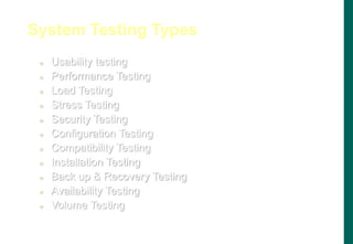
System Testing
Usability Testing
Thetypical aim of usability testing is to cause the application to
fail to meet its usability requirements so that the underlying
defects can be identified, analyzed, fixed, and prevented in the
future.
Performance testing is testing to ensure that the application
response in the limit set by the user.
Performance Testing
Subject the system to extreme pressure in a short
span.
E.g Simultaneous log-on of 500 users
Saturation load of transactions
Stress Testing
363.
Configuration Testing
Configurationtesting is the process of checking the
operation of the software you are testing with all
these various types of hardware.
Compatibility Testing
The purpose of compatibility testing is to evaluate
how well software performs in a particular hardware,
software, operating system, browser or network
environment.
364.
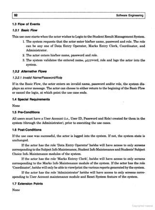
Acceptance Testing
Acceptancetesting may assess the system readiness
for deployment and use
The goal is to establish confidence in the system,
parts of system or non-functional characteristics of
the system
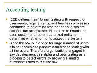
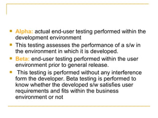
Following are types of Acceptance Testing:
- User Acceptance Testing
- Operational Testing
- Contract and Regulation Acceptance Testing
- Alpha and Beta Testing
365.
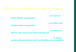
Objectives of DifferentTypes of Testing
In development Testing, main objective is to cause as
many failures as possible.
In Acceptance Testing, main objective is to confirm that
system work as expected.
In Maintenance Testing, main objective is to make sure
that no new errors have been introduced.
In Operational testing, main objective may be to access
system characteristics such as reliability and availability.
366.
Other Testing Types
Otherthan validation activities like unit, integration,
system and acceptance we have the following other
types of testing
Mutation testing
Progressive testing
Regression testing
Retesting
Localization testing
Internationalization testing
367.
Mutation testingis a process of adding known faults
intentionally, in a computer program to monitor the
rate of detection and removal, and estimating the
umber of faults remaining in the program. It is also
called Be-bugging or fault injection.
Mutation testing
368.
Most testcases, unless they are truly throw-away, begin as
progressive test cases and eventually become regression test
cases for the life of the product.
Progressive/Regressive Testing
Regression testing is not another testing activity
It is a re-execution of some or all of the tests developed for a
specific testing activity for each build of the application
Verify that changes or fixes have not introduced new problems
It may be performed for each activity (e.g. unit test, function test,
system test etc)
Regression Testing
369.
Regression Testing
evolveover time
are run often
may become rather large
Why retest?
Because any software product that is actively
used and supported must be changed from time to
time, and every new version of a product should
be retested
Retesting
370.
The processof adapting software to a specific locale,
taking into account, its language, dialect, local
conventions and culture is called localization.
Localization Testing
The process of designing an application so that it can be
adapted to various languages and regions without
engineering changes.
Internationalization Testing
371.
Test Types :The Target of Testing
Testing of functions (functional testing)
- It is the testing of “what” the system does
- Functional testing considers external behavior of the system
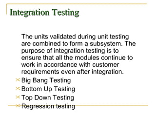
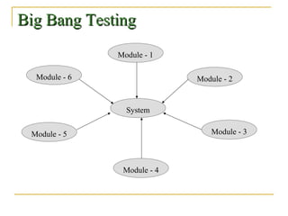
- Functional testing may be performed at all test levels
Testing of software product characteristics (non-functional
testing)
- It is the testing of “How” the system works
- Nonfunctional testing describes the test required to measure
characteristics of systems and s/w that can be quantified on varying
scale
- Non-functional testing may be performed at all levels
372.
Test Types :The Target of Testing
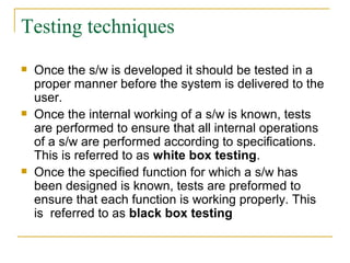
Testing of software structure/architecture (structural testing)
- Structural testing is used in order to help measure the thoroughness of
testing through assessment of coverage of a type of structure
- Structural testing may be performed at all levels.
Testing related to changes (confirmation and regression testing)
- When a defect is detected and fixed then the software should be retested to
confirm that the original defects has been successfully removed. This is
called Confirmation testing
- Regression Testing is the repeated testing of an already tested program,
after modification, to discover any defects as a result of changes.
- Regression Testing may be performed at all levels.
373.
It isthe process of defining a testing project such that
it can be properly measured and controlled
It includes test designing, test strategy, test
requirements and testing resources
Test Planning
374.
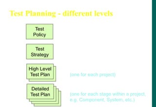
Test Planning -different levels
Test
Policy
Test
Strategy
Company level
High Level
Test Plan
High Level
Test Plan
Project level (IEEE 829)
(one for each project)
Detailed
Test Plan
Detailed
Test Plan
Detailed
Test Plan
Detailed
Test Plan
Test stage level (IEEE 829)
(one for each stage within a project,
e.g. Component, System, etc.)
375.
Parts of TestPlanning
Comm’n
Mgmt
Risk
Mgmt
Test Script
And
Scheduling
Identifying
Test
Deliverables Identifying
Env needs
Identifying
Skill sets /
Trng
Setting
Entry / Exit
Criteria
Deciding
Test
Strategy
Scope
Mgmt
Preparing
A Test
Plan
Test
Planning
Start
Here
376.
Test Planning
TestPlanning is a continuous activity and is performed in all
the life cycle processes and activities
Test Planning activities includes:
- Defining the overall approach
- Integrating and coordinating the testing activities into software life
cycle activities
- Assigning resources for different tasks defined
- Defining the amount, level of detail, structure and templates for test
documentation
- Selecting metrics for monitoring and controlling test preparation
- Making decisions about what to test, what roles will perform the test
activities, when and how test activities should be done, how the test
results will be evaluated and when to stop the testing
377.
Test Planning
ExitCriteria – Defines when to stop testing
Exit criteria may consist of
- Thoroughness measures, such as coverage of code,
functionality or risk
- Estimates of defect density or reliability measures
- Cost
- Residual risk
- Schedules such as those based on time to market
378.
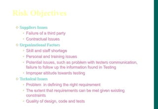
Risk Objectives
SuppliersIssues
• Failure of a third party
• Contractual Issues
Organizational Factors
• Skill and staff shortage
• Personal and training issues
• Potential issues, such as problem with testers communication,
failure to follow up the information found in Testing
• Improper attitude towards testing
Technical Issues
• Problem in defining the right requirement
• The extent that requirements can be met given existing
constraints
• Quality of design, code and tests
379.
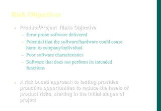
Risk Objectives
Product/ProjectRisks Objective
- Error prone software delivered
- Potential that the software/hardware could cause
harm to company/individual
- Poor software characteristics
- Software that does not perform its intended
functions
A risk based approach to testing provides
proactive opportunities to reduce the levels of
product risks, starting in the initial stages of
project
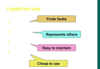
A good testcase
effective
exemplary
evolvable
economic
Finds faults
Represents others
Easy to maintain
Cheap to use
383.
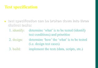
Test specification
testspecification can be broken down into three
distinct tasks:
1. identify: determine „what‟ is to be tested (identify
test conditions) and prioritise
2. design: determine „how‟ the „what‟ is to be tested
(i.e. design test cases)
3. build: implement the tests (data, scripts, etc.)
384.
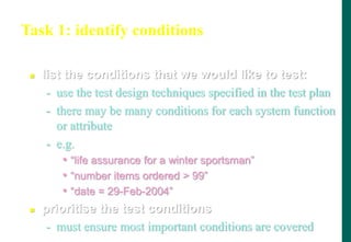
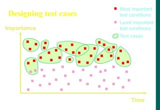
Task 1: identifyconditions
list the conditions that we would like to test:
- use the test design techniques specified in the test plan
- there may be many conditions for each system function
or attribute
- e.g.
• “life assurance for a winter sportsman”
• “number items ordered 99”
• “date = 29-Feb-2004”
prioritise the test conditions
- must ensure most important conditions are covered
(determine „what‟ is to be tested and prioritise)
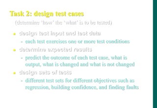
Task 2: designtest cases
design test input and test data
- each test exercises one or more test conditions
determine expected results
- predict the outcome of each test case, what is
output, what is changed and what is not changed
design sets of tests
- different test sets for different objectives such as
regression, building confidence, and finding faults
(determine „how‟ the „what‟ is to be tested)
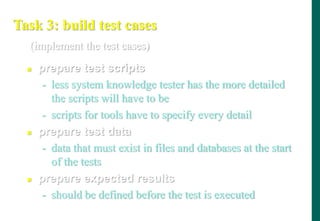
Task 3: buildtest cases
prepare test scripts
- less system knowledge tester has the more detailed
the scripts will have to be
- scripts for tools have to specify every detail
prepare test data
- data that must exist in files and databases at the start
of the tests
prepare expected results
- should be defined before the test is executed
(implement the test cases)
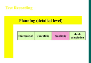
Execution
Execute prescribedtest cases
- most important ones first
- would not execute all test cases if
• testing only fault fixes
• too many faults found by early test cases
• time pressure
- can be performed manually or automated
Test recording 1
The test record contains:
- identities and versions (unambiguously) of
• software under test
• test specifications
Follow the plan
- mark off progress on test script
- document actual outcomes from the test
- capture any other ideas you have for new test cases
- note that these records are used to establish that all
test activities have been carried out as specified
393.
Test recording 2
Compare actual outcome with expected
outcome. Log discrepancies accordingly:
- software fault
- test fault (e.g. expected results wrong)
- environment or version fault
- test run incorrectly
Log coverage levels achieved (for measures
specified as test completion criteria)
After the fault has been fixed, repeat the
required test activities (execute, design, plan)
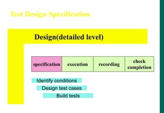
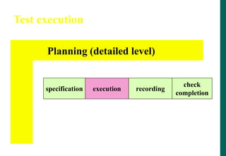
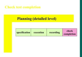
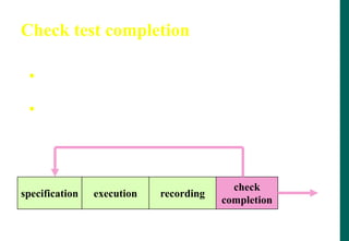
Check test completion
Test completion criteria were specified in the
test plan
If not met, need to repeat test activities, e.g.
test specification to design more tests
specification execution recording
check
completion
Coverage too low
Coverage
OK
396.
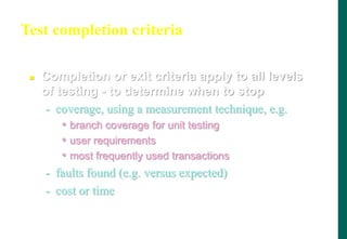
Test completion criteria
Completion or exit criteria apply to all levels
of testing - to determine when to stop
- coverage, using a measurement technique, e.g.
• branch coverage for unit testing
• user requirements
• most frequently used transactions
- faults found (e.g. versus expected)
- cost or time
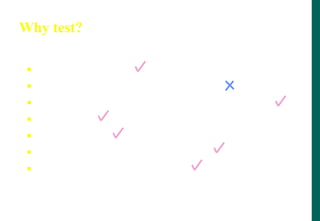
Why test?
buildconfidence
prove that the software is correct
demonstrate conformance to requirements
find faults
reduce costs
show system meets user needs
assess the software quality
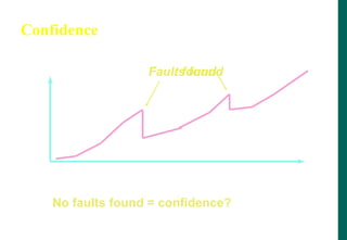
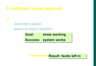
A traditional testingapproach
Show that the system:
- does what it should
- doesn't do what it shouldn't
Fastest achievement: easy test cases
Goal: show working
Success: system works
Result: faults left in
403.
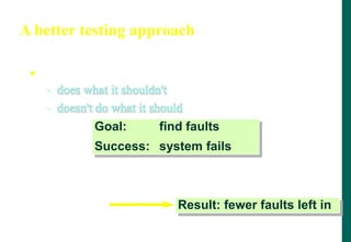
A better testingapproach
Show that the system:
- does what it shouldn't
- doesn't do what it should
Fastest achievement: difficult test cases
Goal: find faults
Success: system fails
Result: fewer faults left in
404.
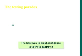
The testing paradox
Purposeof testing: to find faults
The best way to build confidence
is to try to destroy it
Purpose of testing: build confidence
Finding faults destroys confidence
Purpose of testing: destroy confidence
405.
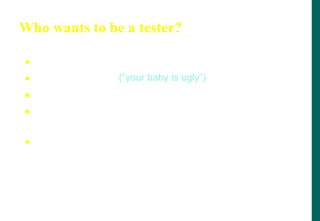
Who wants tobe a tester?
A destructive process
Bring bad news (“your baby is ugly”)
Under worst time pressure (at the end)
Need to take a different view, a different mindset
(“What if it isn‟t?”, “What could go wrong?”)
How should fault information be communicated
(to authors and managers?)
406.
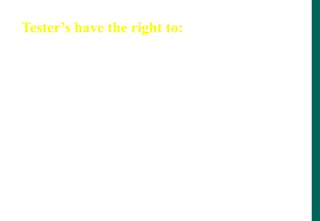
Tester’s have theright to:
- accurate information about progress and changes
- insight from developers about areas of the software
- delivered code tested to an agreed standard
- be regarded as a professional (no abuse!)
- find faults!
- challenge specifications and test plans
- have reported faults taken seriously (non-reproducible)
- make predictions about future fault levels
- improve your own testing process
407.
Testers have responsibilityto:
- follow the test plans, scripts etc. as documented
- report faults objectively and factually (no abuse!)
- check tests are correct before reporting s/w faults
- remember it is the software, not the programmer,
that you are testing
- assess risk objectively
- prioritise what you report
- communicate the truth
408.
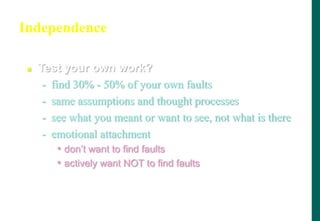
Independence
Test yourown work?
- find 30% - 50% of your own faults
- same assumptions and thought processes
- see what you meant or want to see, not what is there
- emotional attachment
• don‟t want to find faults
• actively want NOT to find faults
409.
Levels of independence
None: tests designed by the person who wrote
the software
Tests designed by a different person
Tests designed by someone from a different
department or team (e.g. test team)
Tests designed by someone from a different
organisation (e.g. agency)
Tests generated by a tool (low quality tests?)
Defect Management
A flawin a system or system component that causes the
system or component to fail to perform its required
function. - SEI
A defect, if encountered during execution, may cause a failure
of the system.
What is definition of defect?
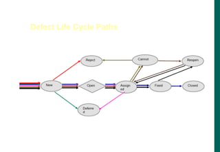
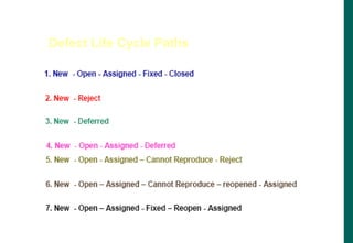
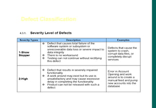
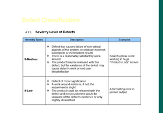
When a testerreports a Defect, it is tracked through the following
stages: New, Open, Fixed, and Closed. A defect may also be
Rejected, or Reopened after it is fixed. A defect may be Deferred
for a look at a later point of time.
By default a defect is assigned the status New.
A quality assurance or project manager reviews the defect, and
determines whether or not to consider the defect for repair. If the
defect is refused, it is assigned the status Rejected.
If the defect is accepted, the quality assurance or project manager
determines a repair priority, changes its status to Open, and
assigns it to a member of the development team.
Defect Life Cycle
416.
A developer repairsthe defect and assigns it the
status Fixed.
Tester retests the application, making sure that the
defect does not recur. If the defect recurs, the quality
assurance or project manager assigns it the status
Reopened.
If the defect is actually repaired, it is assigned the
status Closed.
Defect Life Cycle
How many testersdo we need to
change a light bulb?
None. Testers just noticed that the room was dark.
Testers don't fix the problems, they just find them
422.
Report adefect
The point of writing Problem Reports is to get bugs fixed.
What Do You Do When You Find a defect?
423.
Summary
Datereported
Detailed description
Assigned to
Severity
Detected in Version
Priority
System Info
Status
Reproducible
Detected by
Screen prints, logs, etc.
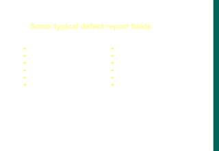
Some typical defect report fields
424.
Project Manager
Executives
Development
Customer Support
Marketing
Quality Assurance
Any member of the Project Team
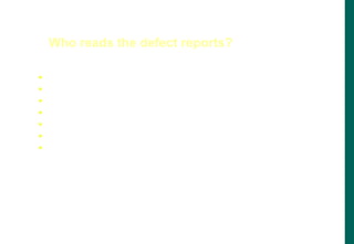
Who reads the defect reports?
Principles of TestAutomation
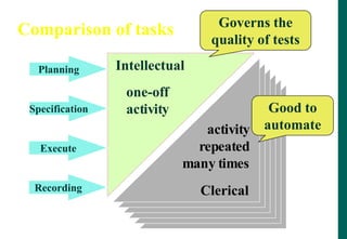
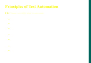
# 1: Choose carefully what to automate
Automate tests for highly visible areas
Minimize automating change-prone areas
Between GUI and non-GUI portion automation, go for automating
non-GUI portions first
Automate tests for dependencies to catch ripple effects early
Automate areas where multiple combos are possible (pros and
cons)
Automate areas that are re-usable
Automate “easy areas” to show low hanging fruits
427.
Principles of TestAutomation
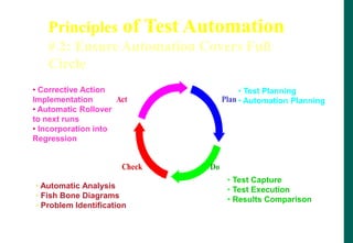
# 2: Ensure Automation Covers Full
Circle
Plan
Do
Check
Act
• Automatic Analysis
• Fish Bone Diagrams
• Problem Identification
• Test Capture
• Test Execution
• Results Comparison
• Test Planning
• Automation Planning
• Corrective Action
Implementation
• Automatic Rollover
to next runs
• Incorporation into
Regression
428.
Compatibility toPlatform
Portability across platforms
Integration with TCDB, DR and SCM
2-way mapping to source code (may not be possible
in services)
Scripting Language
Compatible to Multiple Programming Environments
Configurability
Test Case Reusability
Selective Execution
Smart Comparison
Reliable Support
Current documentation
Principles of Test Automation
# 3: Choose Proper Automation Tool
429.
Resources forInstallation
Resources for ongoing execution
People Resources
Principles of Test Automation
# 4: Plan for Infrastructure
430.
Training
Development
Testing the Tests
Sync-ing with product
version changes
Principles of Test Automation
# 5: Account for Gestation Period
431.
Start small
Don‟t try to automate everything
at the same time
Allow time for evolving standards
Principles of Test Automation
# 6: Run a Trial Calibrate the Tool
• There areplenty of tools available and rarely does one tool meet
all the requirements
• The test tools are expensive (both in upfront costs and running
costs)
• Test tools also require good amount of training and only few
vendors available for training
•Training may not always keep pace with new versions of the tools
• Test tools expect the users to learn new language/scripts and may
not use standard languages/scripts
• Deploying a test tool requires equal amount of effort as deploying a
new product in a company – never underestimate the effort and pain
involved!
Common Experiences in Test Automation
434.
• Migrating fromone test tool to another may be difficult and requires
good amount of effort
• Test tools are one generation behind and may not provide
backward / forward compatibility (eg. JAVA SDK support)
• Good number of test tools requires their libraries linked with
product binaries – Causes portions of the testing to be repeated
after those libraries are removed (eg. Performance)
• Test tools are not 100% cross platform – They are supported only
on some platforms and the sources generated from these tools may
not be compatible on other
• Developing sharewares/public domain test tools may not get same
amount of participation/involvement/support as of
standards/products (eg. As against Linux)
Common Experiences in Test Automation
435.
The experiences
• Testtools may not go through same amount of
evaluation for new requirements (eg Year 2000, 508)
•The test tools increases the system requirements and
requires the H/W and S/W to be upgraded at
compile/run-time
• The test tools are capable of testing only the product,
not the impact because of the product/test tool to the
system or network
• Good number of test tools can‟t differentiate between a
product failure and the test suite failure – Causing
increased analysis time and manual testing
Common Experiences in Test Automation
436.
The experiences
•The testtools may not provide good degree of
trouble shooting / debug/error messages to help
in analysis – Resulting in increased “printf”/log
messages in the test suite
• The test tools determine the results based on
messages and screen co-ordinates at run-time –
Intelligence needed to proactively find out the
changes
Common Experiences in Test Automation
437.
• Automation shouldn‟tbe considered as stop-gap arrangement to
engage test engineers (when no test execution, do automation!). Test
Automation, like any other project, should start with the end in mind
• A separate team in the organization looking at automation
requirements, tool evaluation and developing generic test suites would
add more value (may not always apply to testing services organization)
• Automation doesn‟t stop with automating the test cases alone. The
test suite needs to be linked with other tools for increased
effectiveness (e.g., Test case database, Defect filing, auto mails,
preparing automatic reports, etc)
• Automation doesn‟t stop with recording playing back the user
commands; Automated tool should be intelligent enough to say what
was expected, why a test case failed and give manual steps to
reproduce the problem
Common Pitfalls in Test Automation

![5
Software Engineering (3rd ed.), By K.K Aggarwal Yogesh Singh, Copyright © New Age International Publishers, 2007
}
18.
return 0;
17.
}
16.
}
15.
x[j] = save;
14.
x[i] = x[j];
13.
Save = x[i];
12.
{
11.
if (x[i] x[j])
10.
for (j=1; j=im; j++)
9.
im1=i-1;
8.
{
7.
for (i=2; i=n; i++)
6.
If (n2) return 1;
5.
/*This function sorts array x in ascending order */
4.
int i, j, save, im1;
3.
{
2.
int. sort (int x[ ], int n)
1.
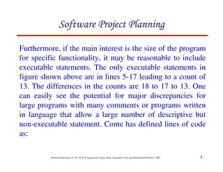
If LOC is simply a count of
the number of lines then
figure shown below contains
18 LOC .
When comments and blank
lines are ignored, the
program in figure 2 shown
below contains 17 LOC.
Lines of Code (LOC)
Size Estimation
123456789A72B8C49AD6EEFE
123456789A72B8C49AD6EEFE
123456789A72B8C49AD6EEFE
123456789A72B8C49AD6EEFE
Fig. 2: Function for sorting an array](https://image.slidesharecdn.com/softwareengineering-250826191237-d21d6ae7/85/SOFTWARE-ENGINEERING-Software-Engineering-3rd-Edition-by-K-K-Aggarwal-Yogesh-Singh-59-320.jpg)
![20
Software Engineering (3rd ed.), By K.K Aggarwal Yogesh Singh, Copyright © New Age International Publishers, 2007
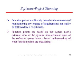
Organizations that use function point methods develop a criterion for
determining whether a particular entry is Low, Average or High.
Nonetheless, the determination of complexity is somewhat
subjective.
FP = UFP * CAF
Where CAF is complexity adjustment factor and is equal to [0.65 +
0.01 x 1Fi]. The Fi (i=1 to 14) are the degree of influence and are
based on responses to questions noted in table 3.
123456789A72B8C49AD6EEFE
123456789A72B8C49AD6EEFE
123456789A72B8C49AD6EEFE
123456789A72B8C49AD6EEFE](https://image.slidesharecdn.com/softwareengineering-250826191237-d21d6ae7/85/SOFTWARE-ENGINEERING-Software-Engineering-3rd-Edition-by-K-K-Aggarwal-Yogesh-Singh-74-320.jpg)

![117
Software Engineering (3rd ed.), By K.K Aggarwal Yogesh Singh, Copyright © New Age International Publishers, 2007
Schedule estimation
Development time can be calculated using PMadjusted as a key factor and the
desired equation is:
100
%
)
(
[ ))]
091
.
0
(
2
.
0
28
.
0
(
nominal
SCED
PM
TDEV B
adjusted ∗
×
= −
+
φ
where 3 = constant, provisionally set to 3.67
TDEVnominal = calendar time in months with a scheduled constraint
B = Scaling factor
PMadjusted = Estimated effort in Person months (after adjustment)
123456789A72B8C49AD6EEFE
123456789A72B8C49AD6EEFE
123456789A72B8C49AD6EEFE
123456789A72B8C49AD6EEFE](https://image.slidesharecdn.com/softwareengineering-250826191237-d21d6ae7/85/SOFTWARE-ENGINEERING-Software-Engineering-3rd-Edition-by-K-K-Aggarwal-Yogesh-Singh-171-320.jpg)
![125
Software Engineering (3rd ed.), By K.K Aggarwal Yogesh Singh, Copyright © New Age International Publishers, 2007
The Norden / Rayleigh Curve
= manpower utilization rate per unit time
a = parameter that affects the shape of the curve
K = area under curve in the interval [0, 4 ]
t = elapsed time
dt
dy
2
2
)
( at
kate
dt
dy
t
m −
=
= --------- (1)
The curve is modeled by differential equation
123456789A72B8C49AD6EEFE
123456789A72B8C49AD6EEFE
123456789A72B8C49AD6EEFE
123456789A72B8C49AD6EEFE](https://image.slidesharecdn.com/softwareengineering-250826191237-d21d6ae7/85/SOFTWARE-ENGINEERING-Software-Engineering-3rd-Edition-by-K-K-Aggarwal-Yogesh-Singh-179-320.jpg)
![126
Software Engineering (3rd ed.), By K.K Aggarwal Yogesh Singh, Copyright © New Age International Publishers, 2007
On Integration on interval [o, t]
Where y(t): cumulative manpower used upto time t.
y(0) = 0
y(4) = k
123456789A72B8C49AD6EEFE
123456789A72B8C49AD6EEFE
123456789A72B8C49AD6EEFE
123456789A72B8C49AD6EEFE
y(t) = K [1-e-at2
] -------------(2)
The cumulative manpower is null at the start of the project, and
grows monotonically towards the total effort K (area under the
curve).](https://image.slidesharecdn.com/softwareengineering-250826191237-d21d6ae7/85/SOFTWARE-ENGINEERING-Software-Engineering-3rd-Edition-by-K-K-Aggarwal-Yogesh-Singh-180-320.jpg)
![127
Software Engineering (3rd ed.), By K.K Aggarwal Yogesh Singh, Copyright © New Age International Publishers, 2007
0
]
2
1
[
2 2
2
2
2
=
−
= −
at
kae
dt
y
d at
a
td
2
1
2
=
“td”: time where maximum effort rate occurs
Replace “td” for t in equation (2)
2
5
.
0
2
2
1
3935
.
0
)
(
)
1
(
1
)
(
2
2
d
t
t
t
a
k
t
y
E
e
K
e
k
t
y
E d
d
=
=
=
−
=
8
8
9
A
B
B
C
D
−
=
= −
123456789A72B8C49AD6EEFE
123456789A72B8C49AD6EEFE
123456789A72B8C49AD6EEFE
123456789A72B8C49AD6EEFE](https://image.slidesharecdn.com/softwareengineering-250826191237-d21d6ae7/85/SOFTWARE-ENGINEERING-Software-Engineering-3rd-Edition-by-K-K-Aggarwal-Yogesh-Singh-181-320.jpg)
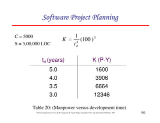
![135
Software Engineering (3rd ed.), By K.K Aggarwal Yogesh Singh, Copyright © New Age International Publishers, 2007
(b) We know
[ ]
2
1
)
( at
e
K
t
y −
−
=
t = 1 year and 2 months
= 1.17 years
041
.
0
)
5
.
3
(
2
1
2
1
2
2
=
×
=
=
d
t
a
[ ]
2
)
17
.
1
(
041
.
0
1
600
)
17
.
1
( −
−
= e
y
= 32.6 PY
123456789A72B8C49AD6EEFE
123456789A72B8C49AD6EEFE
123456789A72B8C49AD6EEFE
123456789A72B8C49AD6EEFE](https://image.slidesharecdn.com/softwareengineering-250826191237-d21d6ae7/85/SOFTWARE-ENGINEERING-Software-Engineering-3rd-Edition-by-K-K-Aggarwal-Yogesh-Singh-189-320.jpg)
![153
Software Engineering (3rd ed.), By K.K Aggarwal Yogesh Singh, Copyright © New Age International Publishers, 2007
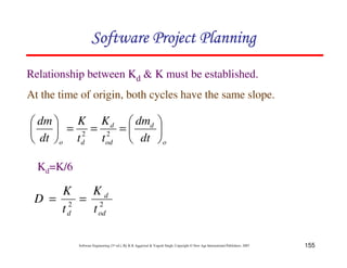
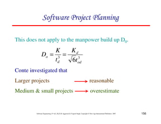
An examination of md(t) function shows a non-zero value of md
at time td.
This is because the manpower involved in design coding is
still completing this activity after td in form of rework due to
the validation of the product.
Nevertheless, for the model, a level of completion has to be
assumed for development.
It is assumed that 95% of the development will be completed
by the time td.
md (t) = 2kdbt e-bt2
yd (t) = Kd [1-e-bt2
]
∴
123456789A72B8C49AD6EEFE
123456789A72B8C49AD6EEFE
123456789A72B8C49AD6EEFE
123456789A72B8C49AD6EEFE](https://image.slidesharecdn.com/softwareengineering-250826191237-d21d6ae7/85/SOFTWARE-ENGINEERING-Software-Engineering-3rd-Edition-by-K-K-Aggarwal-Yogesh-Singh-207-320.jpg)