All about Relational Model of DBMS.

1. Chapter 2: Relational
Model

2. Chapter 2: Relational Model
 Advantages of Relational Model
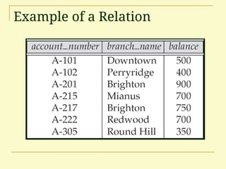
 Structure of Relational Databases
 Fundamental Relational-Algebra-Operations
 Additional Relational-Algebra-Operations
 Extended Relational-Algebra-Operations
 Null Values
 Modification of the Database

3. Advantages of Relational Model
 Simplicity
 Avoids data duplication.
 Avoids inconsistent records.
 Easier to change data
 Easier to change data format
 Data can be added and removed safely
 Easier to maintain security
 Provides a very simple yet powerful way to
represent data

4. Structure of Relational
Databases
 Consists of collection of tables, each of which is
assigned to a unique name.
 A row represent a relationship.
 Table is a collection of relationship
Formally, given sets D1, D2, …. Dn a relation r is a
subset of

5. Example of a Relation

6. Basic Structure
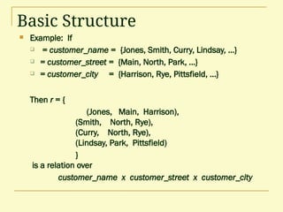
 Example: If
 = customer_name = {Jones, Smith, Curry, Lindsay, …}
 = customer_street = {Main, North, Park, …}
 = customer_city = {Harrison, Rye, Pittsfield, …}
Then r = {
(Jones, Main, Harrison),
(Smith, North, Rye),
(Curry, North, Rye),
(Lindsay, Park, Pittsfield)
}
is a relation over
customer_name x customer_street x customer_city

7. Attribute Types
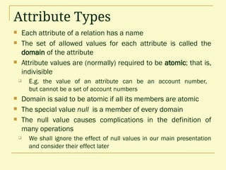
 Each attribute of a relation has a name
 The set of allowed values for each attribute is called the
domain of the attribute
 Attribute values are (normally) required to be atomic; that is,
indivisible
 E.g. the value of an attribute can be an account number,
but cannot be a set of account numbers
 Domain is said to be atomic if all its members are atomic
 The special value null is a member of every domain
 The null value causes complications in the definition of
many operations
 We shall ignore the effect of null values in our main presentation
and consider their effect later

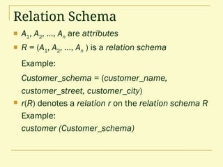
8. Relation Schema
 A1, A2, …, An are attributes
 R = (A1, A2, …, An ) is a relation schema
Example:
Customer_schema = (customer_name,
customer_street, customer_city)
 r(R) denotes a relation r on the relation schema R
Example:
customer (Customer_schema)

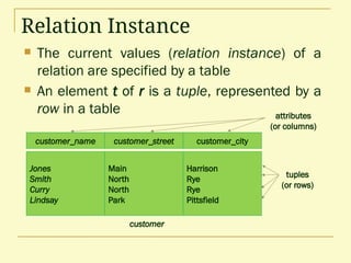
9. Relation Instance
 The current values (relation instance) of a
relation are specified by a table
 An element t of r is a tuple, represented by a
row in a table
Jones
Smith
Curry
Lindsay
customer_name
Main
North
North
Park
customer_street
Harrison
Rye
Rye
Pittsfield
customer_city
customer
attributes
(or columns)
tuples
(or rows)

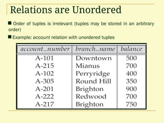
10. Relations are Unordered
 Order of tuples is irrelevant (tuples may be stored in an arbitrary
order)
 Example: account relation with unordered tuples

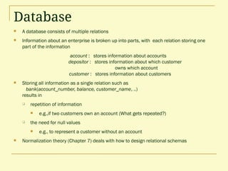
11. Database
 A database consists of multiple relations
 Information about an enterprise is broken up into parts, with each relation storing one
part of the information
account : stores information about accounts
depositor : stores information about which customer
owns which account
customer : stores information about customers
 Storing all information as a single relation such as
bank(account_number, balance, customer_name, ..)
results in
 repetition of information
 e.g.,if two customers own an account (What gets repeated?)
 the need for null values
 e.g., to represent a customer without an account
 Normalization theory (Chapter 7) deals with how to design relational schemas

12. The customer Relation

13. The depositor Relation

14. Keys
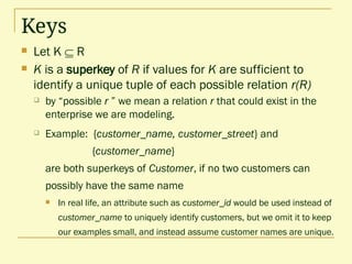
 Let K  R
 K is a superkey of R if values for K are sufficient to
identify a unique tuple of each possible relation r(R)
 by “possible r ” we mean a relation r that could exist in the
enterprise we are modeling.
 Example: {customer_name, customer_street} and
{customer_name}
are both superkeys of Customer, if no two customers can
possibly have the same name
 In real life, an attribute such as customer_id would be used instead of
customer_name to uniquely identify customers, but we omit it to keep
our examples small, and instead assume customer names are unique.

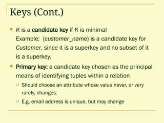
15. Keys (Cont.)
 K is a candidate key if K is minimal
Example: {customer_name} is a candidate key for
Customer, since it is a superkey and no subset of it
is a superkey.
 Primary key: a candidate key chosen as the principal
means of identifying tuples within a relation
 Should choose an attribute whose value never, or very
rarely, changes.
 E.g. email address is unique, but may change

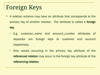
16. Foreign Keys
 A relation schema may have an attribute that corresponds to the
primary key of another relation. The attribute is called a foreign
key.
 E.g. customer_name and account_number attributes of
depositor are foreign keys to customer and account
respectively.
 Only values occurring in the primary key attribute of the
referenced relation may occur in the foreign key attribute of the
referencing relation.

17. Schema diagram

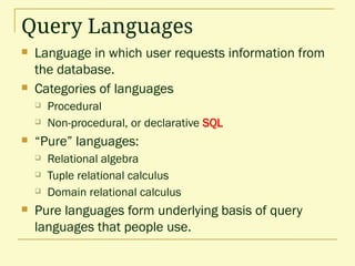
18. Query Languages
 Language in which user requests information from
the database.
 Categories of languages
 Procedural
 Non-procedural, or declarative SQL
 “Pure” languages:
 Relational algebra
 Tuple relational calculus
 Domain relational calculus
 Pure languages form underlying basis of query
languages that people use.

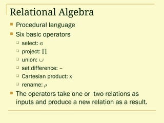
19. Relational Algebra
 Procedural language
 Six basic operators
 select: 
 project: 
 union: 
 set difference: –
 Cartesian product: x
 rename: 
 The operators take one or two relations as
inputs and produce a new relation as a result.

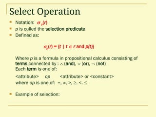
20. Select Operation
 Notation:  p(r)
 p is called the selection predicate
 Defined as:
p(r) = {t | t  r and p(t)}
Where p is a formula in propositional calculus consisting of
terms connected by :  (and),  (or),  (not)
Each term is one of:
<attribute> op <attribute> or <constant>
where op is one of: =, , >, . <. 
 Example of selection:

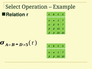
21. Select Operation – Example
Relation r A B C D








1
5
12
23
7
7
3
10
𝝈𝑨=𝑩𝑫 >𝟓( r ) A B C D




1
23
7
10

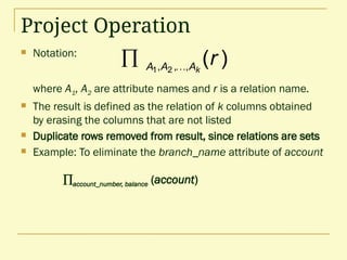
22. Project Operation
 Notation:
where A1, A2 are attribute names and r is a relation name.
 The result is defined as the relation of k columns obtained
by erasing the columns that are not listed
 Duplicate rows removed from result, since relations are sets
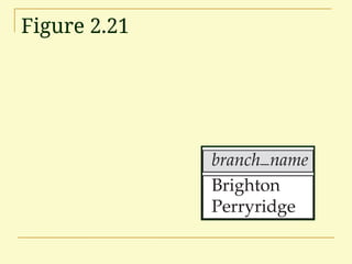
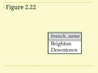
 Example: To eliminate the branch_name attribute of account
account_number, balance (account)
)
(
,
,
, 2
1
r
k
A
A
A 


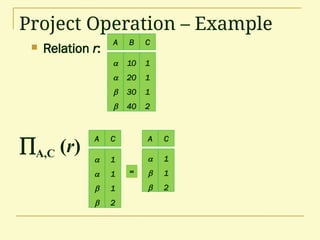
23. Project Operation – Example
 Relation r:
A B C




10
20
30
40
1
1
1
2
A C




1
1
1
2
=
A C



1
1
2
A,C (r)

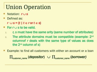
24. Union Operation
 Notation: r  s
 Defined as:
r  s = {t | t  r or t  s}
 For r  s to be valid.
1. r, s must have the same arity (same number of attributes)
2. The attribute domains must be compatible (example: 2nd
columnof r deals with the same type of values as does
the 2nd
column of s)
 Example: to find all customers with either an account or a loan
customer_name (depositor)  customer_name (borrower)

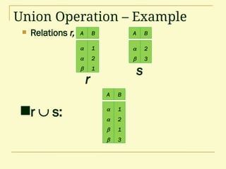
25. Union Operation – Example
 Relations r, s:
r  s:
A B



1
2
1
A B


2
3
r
s
A B




1
2
1
3

26. Set Difference Operation
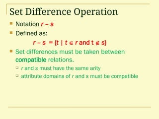
 Notation r – s
 Defined as:
r – s = {t | t  r and t  s}
 Set differences must be taken between
compatible relations.
 r and s must have the same arity
 attribute domains of r and s must be compatible

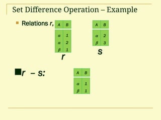
27. Set Difference Operation – Example
 Relations r, s:
r – s:
A B



1
2
1
A B


2
3
r
s
A B


1
1

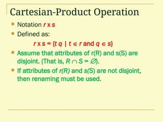
28. Cartesian-Product Operation
 Notation r x s
 Defined as:
r x s = {t q | t  r and q  s}
 Assume that attributes of r(R) and s(S) are
disjoint. (That is, R  S = ).
 If attributes of r(R) and s(S) are not disjoint,
then renaming must be used.

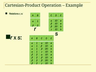
29. Cartesian-Product Operation – Example
 Relations r, s:
r x s:
A B


1
2
A B








1
1
1
1
2
2
2
2
C D








10
10
20
10
10
10
20
10
E
a
a
b
b
a
a
b
b
C D




10
10
20
10
E
a
a
b
b
r
s

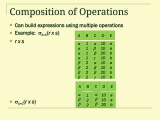
30. Composition of Operations
 Can build expressions using multiple operations
 Example: A=C(r x s)
 r x s
 A=C(r x s)
A B








1
1
1
1
2
2
2
2
C D








10
10
20
10
10
10
20
10
E
a
a
b
b
a
a
b
b
A B C D E



1
2
2



10
10
20
a
a
b

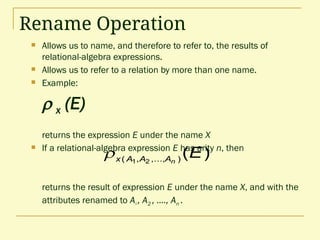
31. Rename Operation
 Allows us to name, and therefore to refer to, the results of
relational-algebra expressions.
 Allows us to refer to a relation by more than one name.
 Example:
 x (E)
returns the expression E under the name X
 If a relational-algebra expression E has arity n, then
returns the result of expression E under the name X, and with the
attributes renamed to A1 , A2 , …., An .
)
(
)
,...,
,
( 2
1
E
n
A
A
A
x


32. 32
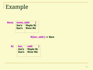
Example
Bars( name, addr )
Joe’s Maple St.
Sue’s River Rd.
R( bar, addr )
Joe’s Maple St.
Sue’s River Rd.
R(bar, addr) := Bars

33. Banking Example
branch (branch_name, branch_city, assets)
customer (customer_name, customer_street,
customer_city)
account (account_number, branch_name,
balance)
loan (loan_number, branch_name, amount)
depositor (customer_name, account_number)
borrower (customer_name, loan_number)

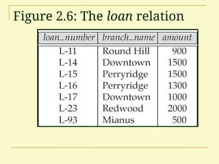
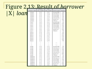
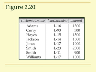
34. Example Queries
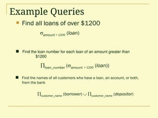
 Find all loans of over $1200
 Find the loan number for each loan of an amount greater than
$1200
amount > 1200 (loan)
loan_number (amount > 1200 (loan))
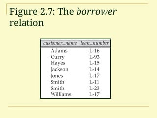
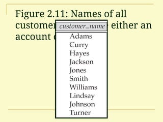
 Find the names of all customers who have a loan, an account, or both,
from the bank
customer_name (borrower)  customer_name (depositor)

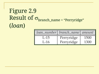
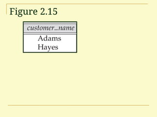
35. Example Queries
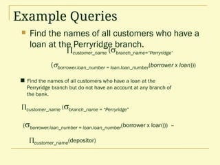
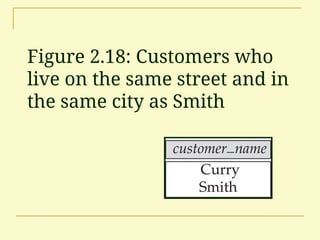
 Find the names of all customers who have a
loan at the Perryridge branch.
 Find the names of all customers who have a loan at the
Perryridge branch but do not have an account at any branch of
the bank.
customer_name (branch_name = “Perryridge”
(borrower.loan_number = loan.loan_number(borrower x loan))) –
customer_name(depositor)
customer_name (branch_name=“Perryridge”
(borrower.loan_number = loan.loan_number(borrower x loan)))

36. Example Queries
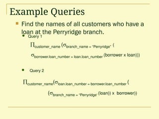
 Find the names of all customers who have a
loan at the Perryridge branch.
 Query 2
customer_name(loan.loan_number = borrower.loan_number (
(branch_name = “Perryridge” (loan)) x borrower))
 Query 1
customer_name (branch_name = “Perryridge” (
borrower.loan_number = loan.loan_number (borrower x loan)))

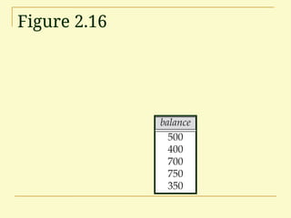
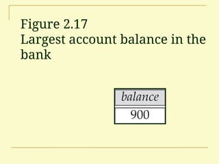
37. Example Queries
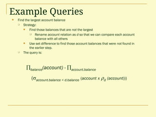
 Find the largest account balance
 Strategy:
 Find those balances that are not the largest
 Rename account relation as d so that we can compare each account
balance with all others
 Use set difference to find those account balances that were not found in
the earlier step.
 The query is:
balance(account) - account.balance
(account.balance < d.balance (account x rd (account)))

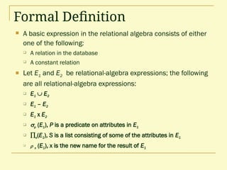
38. Formal Definition
 A basic expression in the relational algebra consists of either
one of the following:
 A relation in the database
 A constant relation
 Let E1 and E2 be relational-algebra expressions; the following
are all relational-algebra expressions:
 E1  E2
 E1 – E2
 E1 x E2
 p (E1), P is a predicate on attributes in E1
 s(E1), S is a list consisting of some of the attributes in E1
  x (E1), x is the new name for the result of E1

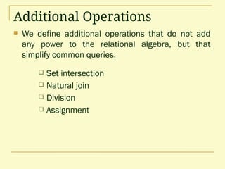
39. Additional Operations
 We define additional operations that do not add
any power to the relational algebra, but that
simplify common queries.
 Set intersection
 Natural join
 Division
 Assignment

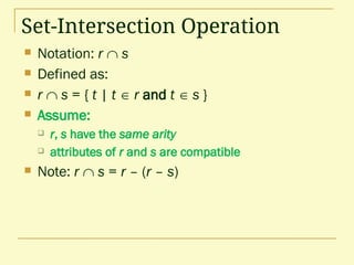
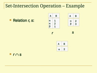
40. Set-Intersection Operation
 Notation: r  s
 Defined as:
 r  s = { t | t  r and t  s }
 Assume:
 r, s have the same arity
 attributes of r and s are compatible
 Note: r  s = r – (r – s)

41. Set-Intersection Operation – Example
 Relation r, s:
 r  s
A B


2
3
A B



1
2
1
r s
A B
 2

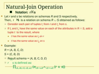
42.  Notation: r s
Natural-Join Operation
 Let r and s be relations on schemas R and S respectively.
Then, r s is a relation on schema R  S obtained as follows:
 Consider each pair of tuples tr from r and ts from s.
 If tr and ts have the same value on each of the attributes in R  S, add a
tuple t to the result, where
 t has the same value as tr on r
 t has the same value as ts on s
 Example:
R = (A, B, C, D)
S = (E, B, D)
 Result schema = (A, B, C, D, E)
 r s is defined as:
r.A, r.B, r.C, r.D, s.E (r.B = s.B r.D = s.D (r x s))

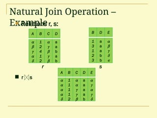
43. Natural Join Operation –
Example
 Relations r, s:
A B





1
2
4
1
2
C D





a
a
b
a
b
B
1
3
1
2
3
D
a
a
a
b
b
E





r
A B





1
1
1
1
2
C D





a
a
a
a
b
E





s
 r s

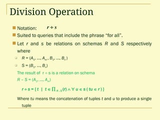
44. Division Operation
 Notation:
 Suited to queries that include the phrase “for all”.
 Let r and s be relations on schemas R and S respectively
where
 R = (A1, …, Am , B1, …, Bn )
 S = (B1, …, Bn)
The result of r  s is a relation on schema
R – S = (A1, …, Am)
r  s = { t | t   R -S (r)   u  s ( tu  r ) }
Where tu means the concatenation of tuples t and u to produce a single
tuple
r  s

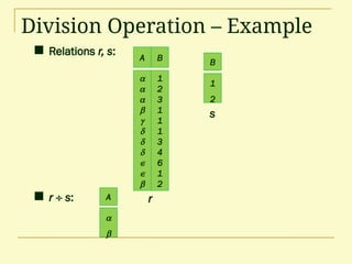
45. Division Operation – Example
 Relations r, s:
 r  s: A
B


1
2
A B











1
2
3
1
1
1
3
4
6
1
2
r
s

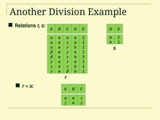
46. Another Division Example
A B








a
a
a
a
a
a
a
a
C D








a
a
b
a
b
a
b
b
E
1
1
1
1
3
1
1
1
 Relations r, s:
 r  s:
D
a
b
E
1
1
A B


a
a
C


r
s

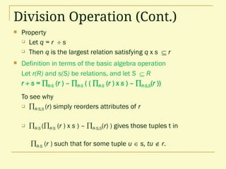
47. Division Operation (Cont.)
 Property
 Let q = r  s
 Then q is the largest relation satisfying q x s  r
 Definition in terms of the basic algebra operation
Let r(R) and s(S) be relations, and let S  R
r  s = R-S (r ) – R-S ( ( R-S (r ) x s ) – R-S,S(r ))
To see why
 R-S,S (r) simply reorders attributes of r
 R-S (R-S (r ) x s ) – R-S,S(r) ) gives those tuples t in
R-S (r ) such that for some tuple u  s, tu  r.

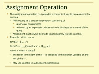
48. Assignment Operation
 The assignment operation () provides a convenient way to express complex
queries.
 Write query as a sequential program consisting of
 a series of assignments
 followed by an expression whose value is displayed as a result of the
query.
 Assignment must always be made to a temporary relation variable.
 Example: Write r  s as
temp1 R-S (r )
temp2  R-S ((temp1 x s ) – R-S,S (r ))
result = temp1 – temp2
 The result to the right of the  is assigned to the relation variable on the
left of the .
 May use variable in subsequent expressions.

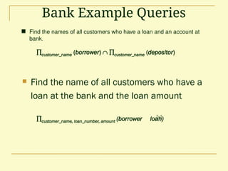
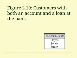
49. Bank Example Queries
 Find the names of all customers who have a loan and an account at
bank.
customer_name (borrower)  customer_name (depositor)
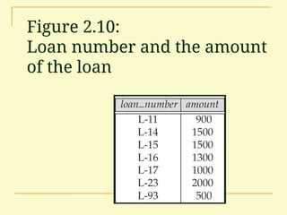
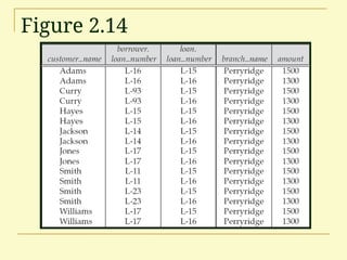
 Find the name of all customers who have a
loan at the bank and the loan amount
customer_name, loan_number, amount (borrower loan)

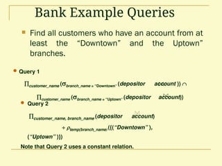
50.  Query 1
customer_name (branch_name = “Downtown” (depositor account )) 
customer_name (branch_name = “Uptown” (depositor account))
 Query 2
customer_name, branch_name (depositor account)
 temp(branch_name) ({(“Downtown” ),
(“Uptown” )})
Note that Query 2 uses a constant relation.
Bank Example Queries
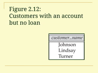
 Find all customers who have an account from at
least the “Downtown” and the Uptown”
branches.

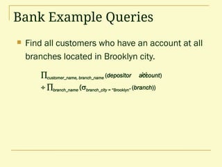
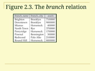
51.  Find all customers who have an account at all
branches located in Brooklyn city.
Bank Example Queries
customer_name, branch_name (depositor account)
 branch_name (branch_city = “Brooklyn” (branch))

52. Extended Relational-Algebra-
Operations
 Generalized Projection
 Aggregate Functions
 Outer Join

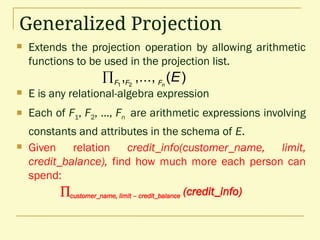
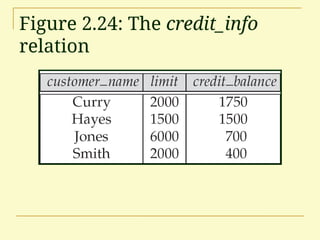
53. Generalized Projection
 Extends the projection operation by allowing arithmetic
functions to be used in the projection list.
 E is any relational-algebra expression
 Each of F1, F2, …, Fn are arithmetic expressions involving
constants and attributes in the schema of E.
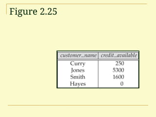
 Given relation credit_info(customer_name, limit,
credit_balance), find how much more each person can
spend:
customer_name, limit – credit_balance (credit_info)
)
(
,...,
, 2
1
E
n
F
F
F


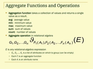
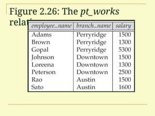
54. Aggregate Functions and Operations
 Aggregation function takes a collection of values and returns a single
value as a result.
avg: average value
min: minimum value
max: maximum value
sum: sum of values
count: number of values
 Aggregate operation in relational algebra
E is any relational-algebra expression
 G1, G2 …, Gn is a list of attributes on which to group (can be empty)
 Each Fi is an aggregate function
 Each Ai is an attribute name
)
(
)
(
,
,
(
),
(
,
,
, 2
2
1
1
2
1
E
n
n
n A
F
A
F
A
F
G
G
G 



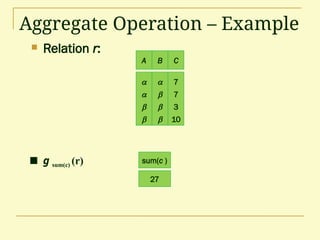
55. Aggregate Operation – Example
 Relation r:
A B








C
7
7
3
10
 g sum(c) (r) sum(c )
27

56. Aggregate Operation – Example
 Relation account grouped by branch-name:
branch_name g sum(balance) (account)
branch_name account_number balance
Perryridge
Perryridge
Brighton
Brighton
Redwood
A-102
A-201
A-217
A-215
A-222
400
900
750
750
700
branch_name sum(balance)
Perryridge
Brighton
Redwood
1300
1500
700

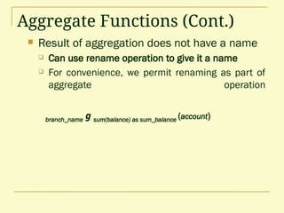
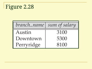
57. Aggregate Functions (Cont.)
 Result of aggregation does not have a name
 Can use rename operation to give it a name
 For convenience, we permit renaming as part of
aggregate operation
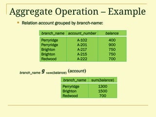
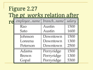
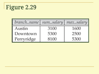
branch_name g sum(balance) as sum_balance (account)

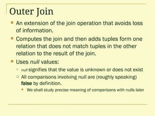
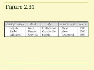
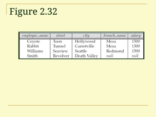
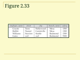
58. Outer Join
 An extension of the join operation that avoids loss
of information.
 Computes the join and then adds tuples form one
relation that does not match tuples in the other
relation to the result of the join.
 Uses null values:

null signifies that the value is unknown or does not exist
 All comparisons involving null are (roughly speaking)
false by definition.
 We shall study precise meaning of comparisons with nulls later

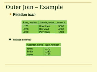
59. Outer Join – Example
 Relation loan
 Relation borrower
customer_name loan_number
Jones
Smith
Hayes
L-170
L-230
L-155
3000
4000
1700
loan_number amount
L-170
L-230
L-260
branch_name
Downtown
Redwood
Perryridge

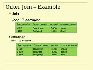
60. Outer Join – Example
 Join
loan borrower
loan_number amount
L-170
L-230
3000
4000
customer_name
Jones
Smith
branch_name
Downtown
Redwood
Jones
Smith
null
loan_number amount
L-170
L-230
L-260
3000
4000
1700
customer_name
branch_name
Downtown
Redwood
Perryridge
 Left Outer Join
loan borrower

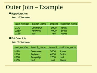
61. Outer Join – Example
loan_number amount
L-170
L-230
L-155
3000
4000
null
customer_name
Jones
Smith
Hayes
branch_name
Downtown
Redwood
null
loan_number amount
L-170
L-230
L-260
L-155
3000
4000
1700
null
customer_name
Jones
Smith
null
Hayes
branch_name
Downtown
Redwood
Perryridge
null
 Full Outer Join
loan borrower
 Right Outer Join
loan borrower

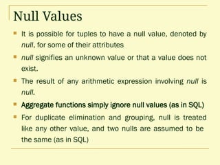
62. Null Values
 It is possible for tuples to have a null value, denoted by
null, for some of their attributes
 null signifies an unknown value or that a value does not
exist.
 The result of any arithmetic expression involving null is
null.
 Aggregate functions simply ignore null values (as in SQL)
 For duplicate elimination and grouping, null is treated
like any other value, and two nulls are assumed to be
the same (as in SQL)

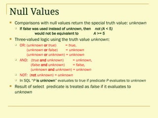
63. Null Values
 Comparisons with null values return the special truth value: unknown
 If false was used instead of unknown, then not (A < 5)
would not be equivalent to A >= 5
 Three-valued logic using the truth value unknown:
 OR: (unknown or true) = true,
(unknown or false) = unknown
(unknown or unknown) = unknown
 AND: (true and unknown) = unknown,
(false and unknown) = false,
(unknown and unknown) = unknown
 NOT: (not unknown) = unknown
 In SQL “P is unknown” evaluates to true if predicate P evaluates to unknown
 Result of select predicate is treated as false if it evaluates to
unknown

64. Modification of the Database
 The content of the database may be modified
using the following operations:
 Deletion
 Insertion
 Updating
 All these operations are expressed using the
assignment operator.

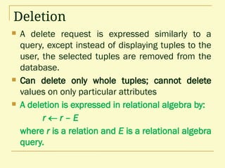
65. Deletion
 A delete request is expressed similarly to a
query, except instead of displaying tuples to the
user, the selected tuples are removed from the
database.
 Can delete only whole tuples; cannot delete
values on only particular attributes
 A deletion is expressed in relational algebra by:
r  r – E
where r is a relation and E is a relational algebra
query.

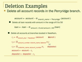
66. Deletion Examples
 Delete all account records in the Perryridge branch.
 Delete all accounts at branches located in Needham.
r1  branch_city = “Needham” (account branch )
r2   account_number, branch_name, balance (r1)
r3   customer_name, account_number (r2 depositor)
account  account – r2
depositor  depositor – r3
 Delete all loan records with amount in the range of 0 to 50
loan  loan – amount 0and amount  50 (loan)
account  account – branch_name = “Perryridge” (account )

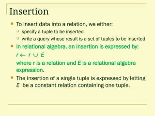
67. Insertion
 To insert data into a relation, we either:
 specify a tuple to be inserted
 write a query whose result is a set of tuples to be inserted
 in relational algebra, an insertion is expressed by:
r  r  E
where r is a relation and E is a relational algebra
expression.
 The insertion of a single tuple is expressed by letting
E be a constant relation containing one tuple.

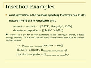
68. Insertion Examples
 Insert information in the database specifying that Smith has $1200
in account A-973 at the Perryridge branch.
 Provide as a gift for all loan customers in the Perryridge branch, a $200
savings account. Let the loan number serve as the account number for the new
savings account.
account  account  {(“A-973”, “Perryridge”, 1200)}
depositor  depositor  {(“Smith”, “A-973”)}
r1  (branch_name = “Perryridge” (borrower loan))
account  account  loan_number, branch_name, 200 (r1)
depositor  depositor  customer_name, loan_number (r1)

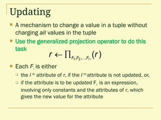
69. Updating
 A mechanism to change a value in a tuple without
charging all values in the tuple
 Use the generalized projection operator to do this
task
 Each Fi is either
 the I th
attribute of r, if the I th
attribute is not updated, or,
 if the attribute is to be updated Fi is an expression,
involving only constants and the attributes of r, which
gives the new value for the attribute
)
(
,
,
,
, 2
1
r
r l
F
F
F 



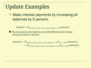
70. Update Examples
 Make interest payments by increasing all
balances by 5 percent.
 Pay all accounts with balances over $10,000 6 percent interest
and pay all others 5 percent
account   account_number, branch_name, balance * 1.06 ( BAL  10000 (account ))
  account_number, branch_name, balance * 1.05 (BAL  10000 (account))
account   account_number, branch_name, balance * 1.05 (account)

71. End of Chapter 2

72. Figure 2.3. The branch relation

73. Figure 2.6: The loan relation

74. Figure 2.7: The borrower
relation

75. Figure 2.9
Result of branch_name = “Perryridge”
(loan)

76. Figure 2.10:
Loan number and the amount
of the loan

77. Figure 2.11: Names of all
customers who have either an
account or an loan

78. Figure 2.12:
Customers with an account
but no loan

79. Figure 2.13: Result of borrower
|X| loan

80. Figure 2.14

81. Figure 2.15

82. Figure 2.16

83. Figure 2.17
Largest account balance in the
bank

84. Figure 2.18: Customers who
live on the same street and in
the same city as Smith

85. Figure 2.19: Customers with
both an account and a loan at
the bank

86. Figure 2.20

87. Figure 2.21

88. Figure 2.22

89. Figure 2.23

90. Figure 2.24: The credit_info
relation

91. Figure 2.25

92. Figure 2.26: The pt_works
relation

93. Figure 2.27
The pt_works relation after
regrouping

94. Figure 2.28

95. Figure 2.29

96. Figure 2.30
The employee and ft_works
relations

97. Figure 2.31

98. Figure 2.32

99. Figure 2.33

100. Figure 2.34