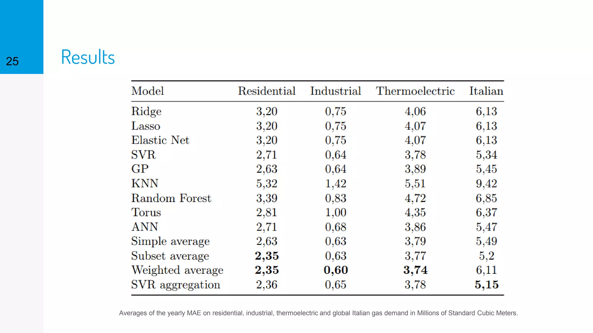
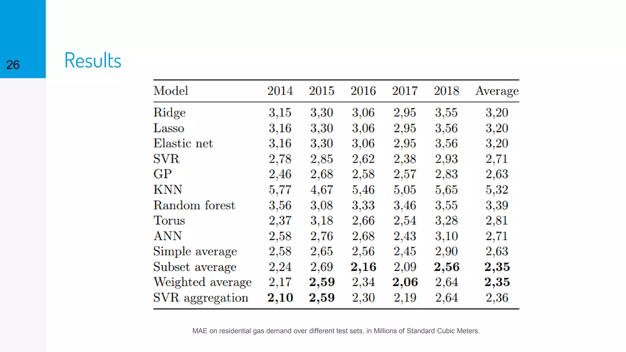
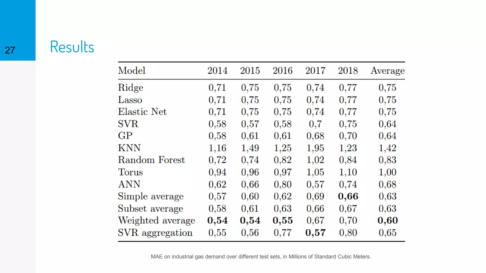
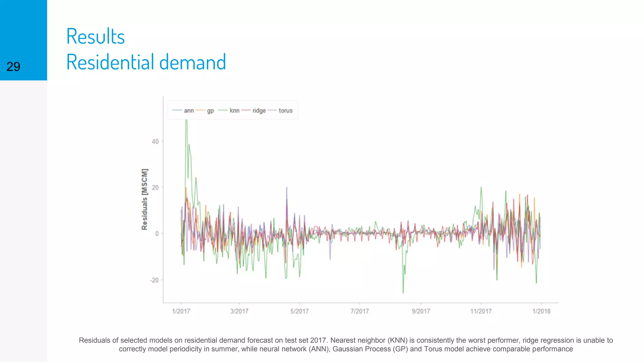
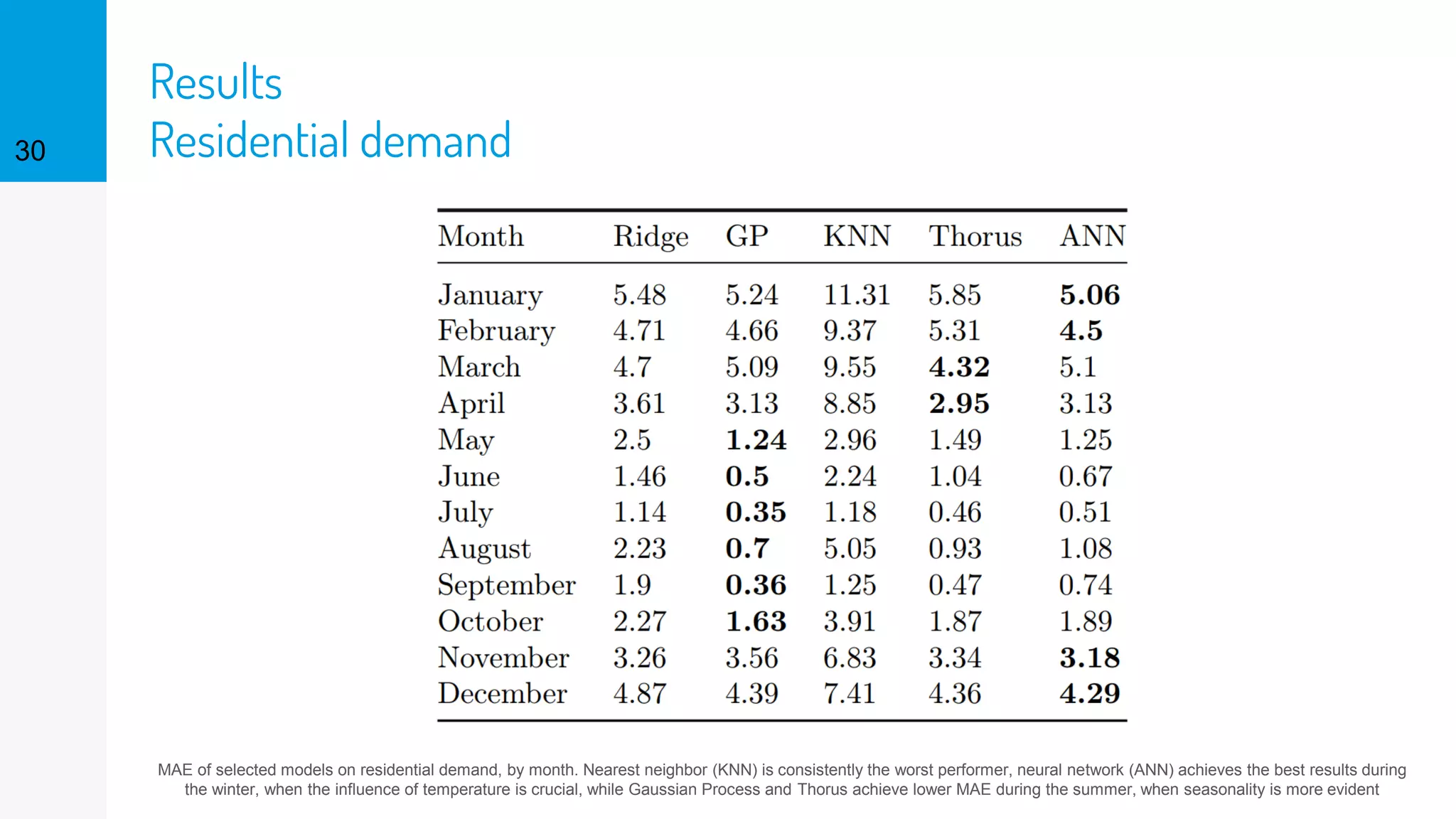
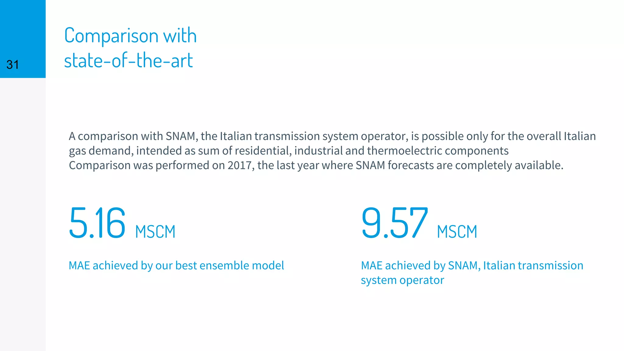
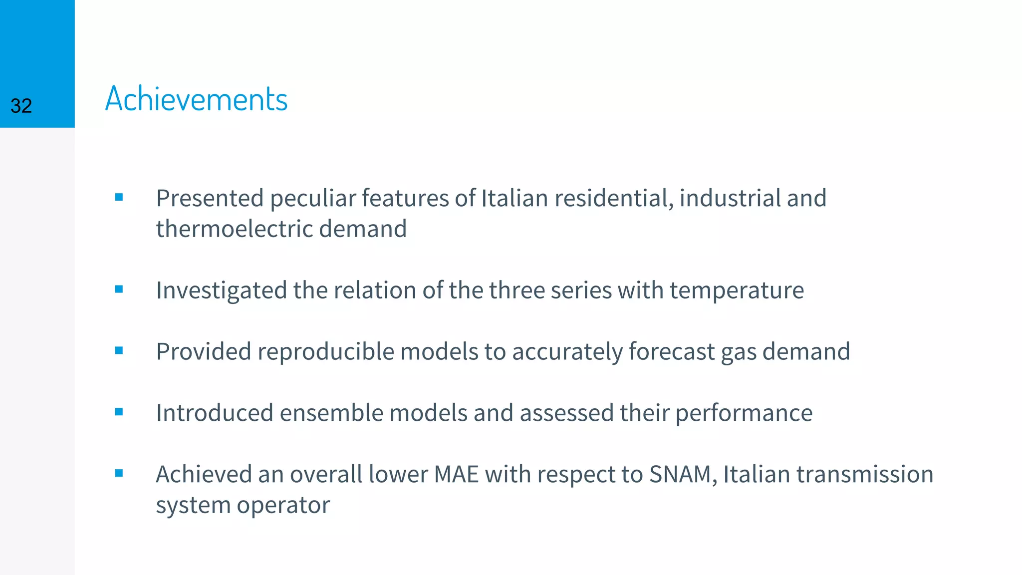
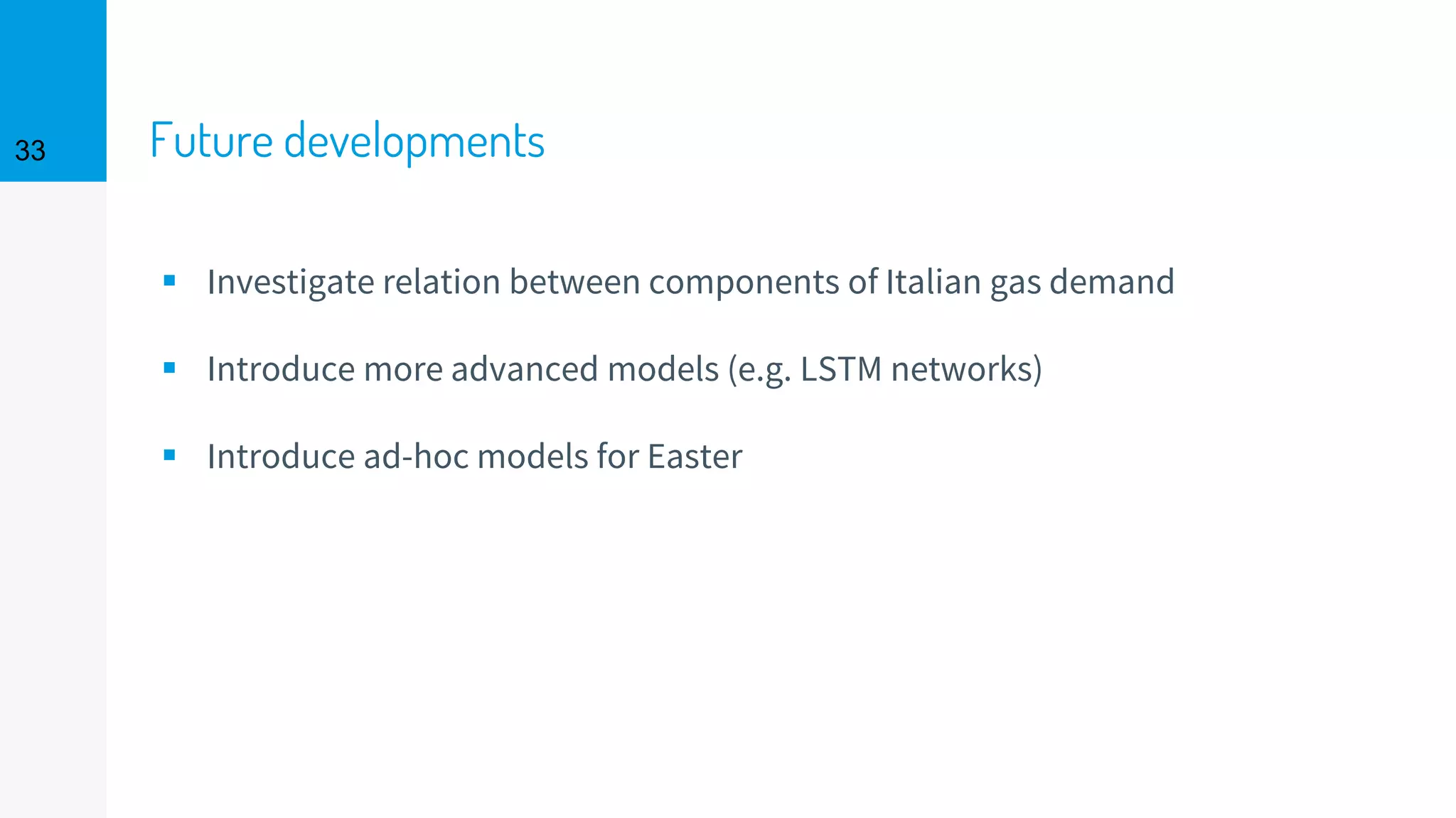
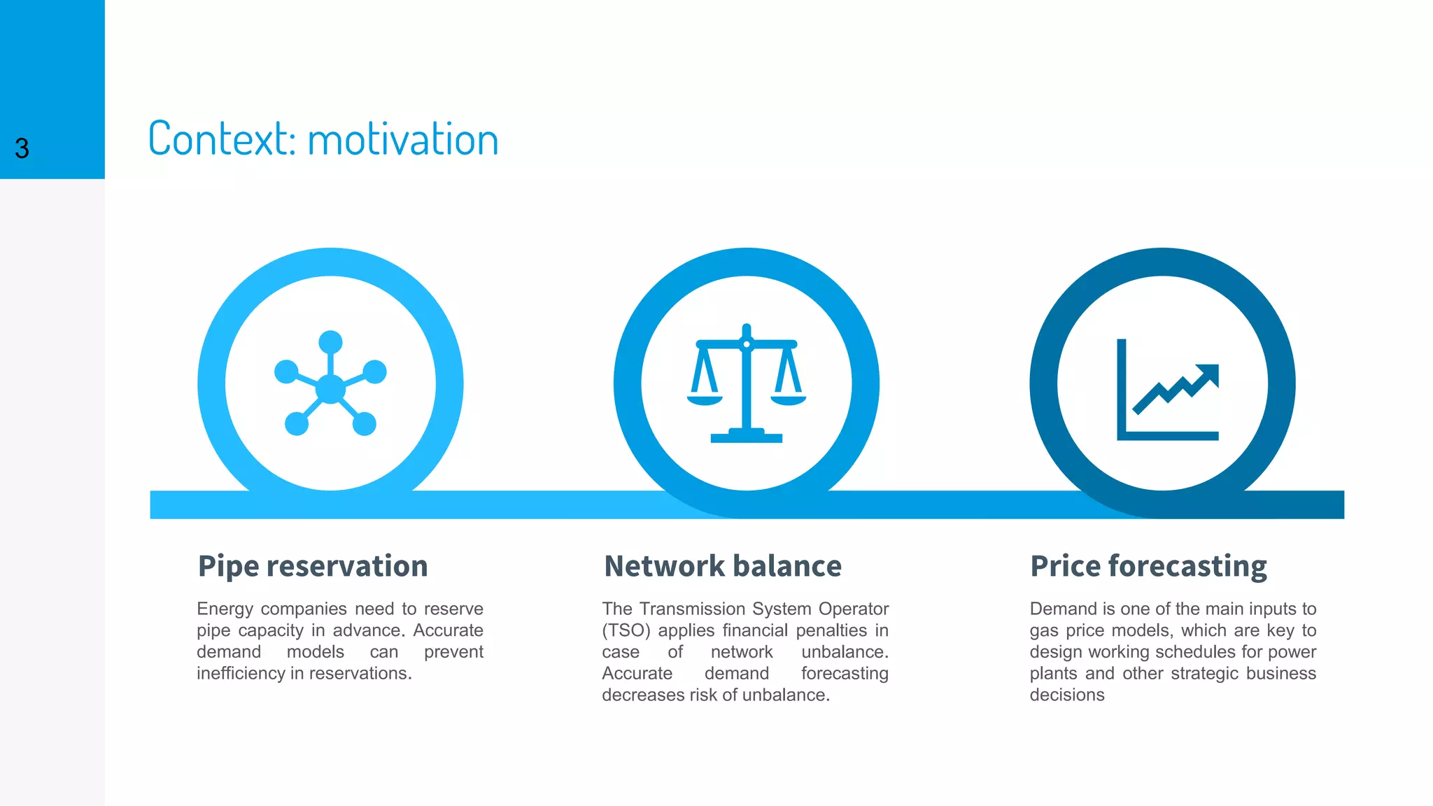
This document discusses the need for accurate short-term forecasting of Italian gas demand, highlighting its importance for gas companies in making informed decisions regarding pipe reservations and mitigating financial penalties due to network imbalances. The authors explore various modeling approaches and present results from predictive models for residential, industrial, and thermoelectric gas demand, noting improved performance compared to existing methods. Future work is suggested to enhance forecasting models and investigate interdependencies among demand components.

1. Short-term forecasting
of Italian gas demand
EmanueleFabbiani
Andrea Marziali
Giuseppe De Nicolao
Energy Finance Italia 4,
Milan, 4-5 February 2019

2. Context: actors2
➢ A2A needs accurate models for Italian
gas demand
➢ University of Pavia has a strong
expertise on time series forecasting

3. Context: motivation3
Pipe reservation
Energy companies need to reserve
pipe capacity in advance. Accurate
demand models can prevent
inefficiency in reservations.
Network balance
The Transmission System Operator
(TSO) applies financial penalties in
case of network unbalance.
Accurate demand forecasting
decreases risk of unbalance.
Price forecasting
Demand is one of the main inputs to
gas price models, which are key to
design working schedules for power
plants and other strategic business
decisions

4. Context: Italian gas demand4
0
10
20
30
40
50
60
70
80
2015 2016 2017
Demand[BSCM]
Residential Industrial Thermoelectic
Source: SNAM Rete Gas, http://pianodecennale.snamretegas.it/it/domanda-offerta-di-gas-in-italia/domanda-di-gas-naturale.html

5. Problem statement5
Given:
▪ Daily Italian residential, industrial and thermoelectric demand from 2007 to 2018
▪ Forecasts of average daily temperature for Northern Italy from 2007 to 2018
▪ Actual average daily temperature for Northern Italy from 2015 to 2017
Perform:
▪ Day-ahead prediction of residential, industrial and thermoelectric gas demand
▪ Day-ahead prediction of Italian gas demand

6. Literature review6
Reviews:
▪ Božidar Soldo, Forecasting natural gas consumption, 2012
▪ Dario Šebalj, Josip Mesarić, and Davor Dujak, Predicting natural gas consumption – a literature
review, 2017
Country-wide forecasting:
▪ Lixing Zhu, MS Li, QH Wu, and L Jiang, Short-term natural gas demand prediction based on support
vector regression with false neighbours filtered, 2015
▪ Joannis P Panapakidis and Athanasios S Dagoumas, Day-ahead natural gas demand forecasting
based on the combination of wavelet transform and anfis/genetic algorithm/neural network model,
2017
Focus on Italy:
▪ Lorenzo Baldacci, Matteo Golfarelli, Davide Lombardi and Franco Sami, Natural gas consumption
forecasting for anomaly detection, 2016

7. Literature review7
Missing:
▪ Country-wide forecasting focusing on Italian demand
▪ Study of the features of Italian residential, industrial and thermoelectric demands

8. Approach8
Exploratory
analysis
STEP 1
Feature
engineering
STEP 2
Modelling
STEP 3
Validation
STEP 4

9. Exploratory analysis
Residential demand9
Italian daily residential gas demand (RGD).

10. Exploratory analysis
Residential demand10
Italian daily residential gas demand (RGD). Time series are shifted to align weekdays: weekly periodicity is particularly visible in summer.
The yearly seasonal variation is mostly explained by heating requirements. In the inset, two weeks of July’s demand data are zoomed

11. Exploratory analysis
Residential demand11
Periodogram of Italian daily residential gas demand (RGD). Left panel: periods from 0 to 8 days; right panel: periods from 0 to 500 days. The yearly periodicity is highlighted by
peaks at 365.25 days, while the weekly one by the smaller spike at a period of 7 days. Other notable values are caused by harmonics

12. Similar day12

13. Exploratory analysis
Residential demand13
Scatter plots between residential gas demand (RGD) and potential features to be used for its prediction. It is possible to note that RGD at times t-1, t-7 and sim(t) is highly
correlated with RGD at time t. Moreover, RGD(t-1)-RGD(sim(t-1)) appears to be a good proxy of RGD(t) – RGD(sim(t))

14. Exploratory analysis
Residential demand14
Relation between Italian daily residential gas demand (RGD) and temperature. Left panel: scatter plot of daily RGD vs average daily temperature. Right panel: scatter plot of
daily RGD vs HDD. Inset: HDD as a function of the temperature. The relation between HDD and RGD is approximately linear

15. Exploratory analysis
Residential demand15
Time series of residential gas demand (RGD) and Heating Day Degrees (HDD) in 2017. The instantaneous correlation between the two series is apparent

16. Exploratory analysis
Industrial demand16
Italian daily industrial gas demand (IGD). The decrease in average value in 2009 is an effect of the economic crisis started in 2008, while negative peaks are Christmas, Easter
and summer holidays

17. Exploratory analysis
Industrial demand17
Periodogram of Italian daily industrial gas demand (IGD). Left panel: periods from 0 to 8 days; right panel: periods from 0 to 500 days. Notably, the peak ascribable to weekly
periodicity is here higher than the one produced by yearly seasonality

18. Exploratory analysis
Industrial demand18
Relation between Italian daily industrial gas demand (IGD) and temperature. Left panel: scatter plot of daily IGD vs average daily temperature. Right panel: scatter plot of daily
IGD vs HDD. The relation between IGD and temperature looks linear in the whole range of values, thus the introduction of HDD does not increase the correlation

19. Exploratory analysis
Thermoelectric demand19
Italian daily thermoelectric gas demand (TGD). The decreasing trend from 2010 to 2014 is explained by the rise of renewable power sources, which slowed down since 2015

20. Exploratory analysis
Thermoelectric demand20
Periodogram of Italian daily thermoelectric gas demand (TGD). Left panel: periods from 0 to 8 days; right panel: periods from 0 to 500 days. Due to several exogenous factors
which affect TGD (like power price and gas price), yearly periodicity is less important than in IGD and RGD

21. Exploratory analysis
Industrial demand21
Relation between Italian daily thermoelectric gas demand (TGD) and temperature. Left panel: scatter plot of daily TGD vs average daily temperature. Right panel: scatter plot of
daily TGD vs Heating and Cooling Day Degrees (HCDD), defined as HCDD = |temperature -16°C|. The influence of temperature on TGD is similar to the one on power demand

22. Exploratory analysis
Final features22

23. Modelling
Basic models:
▪ Regularized linear models: lasso, ridge, elastic net
▪ Non-linear models: Torus model, support vector regression, random forest, fully-connected neural
networks
▪ Non-parametric models: Gaussian process, nearest neighbours
Ensemble models
▪ Simple average
▪ Weighted average
▪ Average on an optimized subset of basic forecasts
▪ Support vector regression
23

24. Experiments24
TRAIN VALIDATION TEST
1 year1 yearall data previous to validation
▪ Five one-year-long test sets, from 2014 to 2018, to assess out-of-sample performance
▪ To each test set is associated a validation set, covering the previous year, to train ensemble models
▪ All the data previous to the start of the validation set are included in train set of basic models
▪ Standalone basic models (i.e. basic models not used for ensembling) are trained on the union of
train and validation sets
TRAIN TESTBasic models
Ensemble models

25. Results25
Averages of the yearly MAE on residential, industrial, thermoelectric and global Italian gas demand in Millions of Standard Cubic Meters.

26. Results26
MAE on residential gas demand over different test sets, in Millions of Standard Cubic Meters.

27. Results27
MAE on industrial gas demand over different test sets, in Millions of Standard Cubic Meters.

28. Results28
MAE on thermoelectric gas demand over different test sets, in Millions of Standard Cubic Meters.

29. Results
Residential demand29
Residuals of selected models on residential demand forecast on test set 2017. Nearest neighbor (KNN) is consistently the worst performer, ridge regression is unable to
correctly model periodicity in summer, while neural network (ANN), Gaussian Process (GP) and Torus model achieve comparable performance

30. Results
Residential demand30
MAE of selected models on residential demand, by month. Nearest neighbor (KNN) is consistently the worst performer, neural network (ANN) achieves the best results during
the winter, when the influence of temperature is crucial, while Gaussian Process and Thorus achieve lower MAE during the summer, when seasonality is more evident

31. Comparison with
state-of-the-art31
9.57 MSCM
MAE achieved by SNAM, Italian transmission
system operator
5.16 MSCM
MAE achieved by our best ensemble model
A comparison with SNAM, the Italian transmission system operator, is possible only for the overall Italian
gas demand, intended as sum of residential, industrial and thermoelectric components
Comparison was performed on 2017, the last year where SNAM forecasts are completely available.

32. Achievements
▪ Presented peculiar features of Italian residential, industrial and
thermoelectric demand
▪ Investigated the relation of the three series with temperature
▪ Provided reproducible models to accurately forecast gas demand
▪ Introduced ensemble models and assessed their performance
▪ Achieved an overall lower MAE with respect to SNAM, Italian transmission
system operator
32

33. Future developments
▪ Investigate relation between components of Italian gas demand
▪ Introduce more advanced models (e.g. LSTM networks)
▪ Introduce ad-hoc models for Easter
33

34. Acknowledgements34

35. ”
Thank you!
35