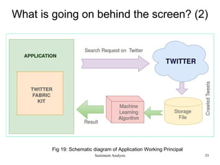
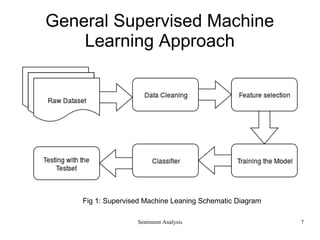
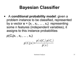
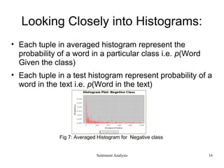
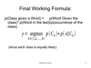
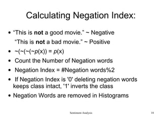
The document presents a comprehensive overview of sentiment analysis on Twitter, discussing its methodology, datasets, and various models such as k-nearest neighbors and recurrent neural networks. It emphasizes data preprocessing, cleaning steps, and the implementation of advanced models like LSTM for improved accuracy. The project highlights practical applications, future improvements, and references to related works in the field.

1. SENTIMENT ANALYSIS
ON TWITTER
PRESENTED BY : SUBARNO PAL
SUVAM MONDAL
SOURAV KAR
SOURAV SENAPATI
SUBHAJIT GHOSH
DEPARTMENT : CSE
UNDER GUIDANCE OF : Dr. SOUMADIP GHOSH
PROJECT : CS892CS892
ACADEMY OF TECHNOLOGY
Date: 01/06/2017
1Sentiment Analysis

2. Sentiment Analysis
What is Sentiment Analysis?

Computational process for identifying and
categorizing opinions expressed in a piece of
text

Determining the writer's attitude towards a
particular topic, product, etc. is positive,
negative

Extract Sentiment of a Text

“Supervised Machine Learning Problem”
2

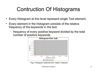
3. Sentiment Analysis
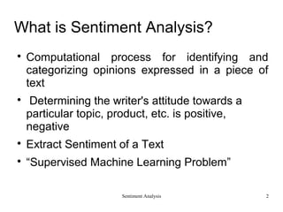
Related Works(1)

Mehto A. proposed a ‘Lexicon based approach for Sentiment Analysis’
based on an aspect catalogue. [1]
 The keywords present in aspect catalogue identified in those
sentences in which features of any product are mentioned.
 Based on these sentences weighted features from the aspect
catalogue are summed up to find the sentiment of the text.

Nizam and AkÕn unsupervised learning for sentiment classification in
Turkish. [2]
 Used tweet words as features and tweet data were clustered in
positive, negative and neutral labelled classes.
 Then, this dataset is used to detect classification accuracy with NB,
DT and KNN algorithms.
3

4. Sentiment Analysis
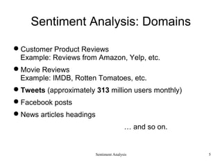
Related Works(2)

In a recent work cited as “A New Approach to Target Dependent
Sentiment Analysis with Onto-Fuzzy Logic”.[3]
 Hash-tagged words of twitter are given special preference for
determining sentiment of the text.
 Hash-tags Category: Topic hash tags , sentiment hash-tags
and sentiment-topic hash tags .

Chikersal P. et. al. developed by Rule-based Classified
combining with Supervised Learning.[4]
 The Support Vector Machine (SVM) is trained on semantic,
dependency, and sentiment lexicon based features. By this it
identify +ve, –ve & neutral keyword.
4

5. Sentiment Analysis
Sentiment Analysis: Domains
Customer Product Reviews
Example: Reviews from Amazon, Yelp, etc.
Movie Reviews
Example: IMDB, Rotten Tomatoes, etc.
Tweets (approximately 313 million users monthly)
Facebook posts
News articles headings
… and so on.
5

6. Sentiment Analysis
Quirks of Tweets:
Informal, and short (140 characters)
Abbreviations and shortenings.
 Spelling mistakes and creative spellings.
Special strings
Hashtags, emoticons, conjoined words.
High volume, 500 million tweets posted every
day.
6

7. Sentiment Analysis
General Supervised Machine
Learning Approach
Fig 1: Supervised Machine Leaning Schematic Diagram
7

8. Dataset Description
• Mainly consisting of TWO classes:
• Positive Class – 1
• Negative Class – 0
• Labeled datasets used for Training
• Training dataset used in applications are
manually labeled Tweets, for testing and result
generation real time data is crawled from Twitter
Sentiment Analysis 8

9. Sentiment Analysis
Data Cleaning and Preprocessing

Removal of the punctuation marks.

Tokenization of the text into single words.

Converting the complete text into single case (upper or
lower case).

Considering only one instance of a particular word.
(discarding the remaining repetitions of the word).
Before After
“A very, very, slow-moving,
aimless movie about a
distressed, drifting young man.”
‘a’ , ‘very’ , ‘slow-moving’ ,
‘aimless’ , ‘movie’ , ‘about’ ,
‘distressed’ , ‘drifting’ ,
‘young’ and ‘man’
9

10. Sentiment Analysis
Data Selection

Selection of tokens are most frequent and probably has more
effect on the sentiment of the text(1000 keywords).

The tokens/keywords are divided into the following 2 sections:-
− Negative Keywords: All available prepositions,
conjunctions and articles.
− Positive Keywords: All remaining words after discarding
the negative keywords.
Before After
‘a’ , ‘very’ , ‘slow-moving’ ,
‘aimless’ , ‘movie’ , ‘about’ ,
‘distressed’ , ‘drifting’ ,
‘young’ and ‘man’
‘very’ , ‘slow-moving’ ,
‘aimless’ , ‘movie’ ,
‘distressed’ , ‘drifting’ ,
‘young’ and ‘man’
10

11. Sentiment Analysis
Contruction Of Histograms

Every Histogram at this level represent single Test element.

Every element in the histogram consists of the relative
frequency of the keywords in the text.
− frequency of every positive keyword divided by the total
number of positive keywords
Fig 2: Histogram obtained from Table 2. features
11

12. Sentiment Analysis
Averaged Histogram

Every Histogram at
represents a Class
present.

Histograms of every
particular class is
added up and divided
by the number of
training elements of
that class in the set.
Fig 3: Histogram of +ve and -ve Class
12

13. Sentiment Analysis
Workflow
Fig 5: Workflow design of the System
13

14. Sentiment Analysis
k-Nearest Neighbour Classifier
 Computing the distance between
the feature vectors of test
histogram and the avg. histograms
 Least distant class is predicted as
the class of the element
 Manhattan Distance:
 Euclidian Distance:
 Result: 74% (approx)
Fig 6: KNN Classifier
A,B – Training set
C – Testing set
14
d( x , y)=∑
i=1
n
| pi−qi|
d( x , y)=∑
i=1
n
| pi
2
−qi
2
|

15. Bayesian Classifier
• A conditional probability model: given a
problem instance to be classified, represented
by a vector x = {x1 , x2 , ... , xn} representing
some n features (independent variables), it
assigns to this instance probabilities
p(Ck|x1 , x2 , ... , xn)
p(Ci| x)=
p( x|Ci) p(Ci )
p( x )
Sentiment Analysis 15

16. Looking Closely into Histograms:
• Each tuple in averaged histogram represent the
probability of a word in a particular class i.e. p(Word
Given the class)
• Each tuple in a test histogram represent probability of a
word in the text i.e. p(Word in the text)
Fig 7: Averaged Histogram for Negative class
Sentiment Analysis 16

17. Final Working Formula:
p(Class given a Word) = p(Word Given the
class)* p(Word in the text)/p(occurrence of the
class)
(since each class is equally likely)
y= argmax
k∈{1,2,..., K}
p(Ck )∗p(x|Ck )
Sentiment Analysis 17

18. Calculating Negation Index:
• “This is not a good movie.” ~ Negative
“This is not a bad movie.” ~ Positive
• ~(~(~(~p(x)) = p(x)
• Count the Number of Negation words
• Negation Index = #Negation words%2
• If Negation Index is '0' deleting negation words
keeps class intact, '1' inverts the class
• Negation Words are removed in Histograms
Sentiment Analysis 18

19. Bayesian Model Implementation:
For Training part:
• Negation Index 1 inverts the class while training & negation
0 keeps same class.
For Testing Part and Result Generation:
• Negation words are deleted from the text
• Bayesian classifier is used for prediction
• Negation Index 1 inverts the class & negation 0 keeps
prediction.
• Result: 80% and above (approx)
Sentiment Analysis 19

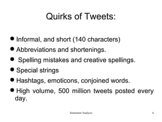
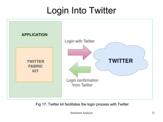
20. Recurrent Neural Network
Sentiment Analysis 20
• Recurrent Neural Network has the
histograms as inputs and it passes through
one hidden layer and finally output layer
gives the result
• Activation function tanh is used
• Weight and bias matrix continuously
updates matching the output in
subsequent steps (6000-10000)
•
• . varies [-1,1]
• Accuracy : above 75% (approx)
• Vanishing gradient problem
hW ,b( x )=f (WT
x )=f ( ∑
i=1
1000
Wi xi+b)
f ( x)=tanh ( x)=
e
x
−e
−x
ex
+e−x
Fig 8: Recurrent Neural Net

21. Long Short Term Memory(LSTM)
•Input gate layer
•Forget gate and tanh layer
•Cell state update layer
•Output layer
Sentiment Analysis 21
f t=σ(Wf .[ht−1 ,xt ]+bf )
it=σ(Wi .[ht−1 ,xt ]+bi )
~
Ct=tanh(WC.[ht−1,xt]+bc )
Ct=ft∗Ct−1+it∗
~
Ct
ot=σ(Wo[ht−1, xt ]+bo)
ht=ot *tanh(Ct )
Fig 9: RNN & LSTM unfolded [6]

22. LSTM Network Implementation
Input_1: Layer that represents a particular
input port in the network.
Embedding_1: Turn positive integers
(indexes) into dense vectors of fixed size,
with dropout rate 0.2.
LSTM_1: LSTM Layer. Dropout rates for
gate and itself is 0.2. Activation function
tanh is used.
Dense_1: Just your regular densely-
connected nn layer. Activation function
sigmoid is used.
Output_1: Layer that represents a
particular output port in the network.
Sentiment Analysis 22
Fig 10: LSTM Flowchart [7]

23. LSTM Results
Sentiment Analysis 23
Fig 11: LSTM Results Analysis

24. Desktop Application
Implementation
Sentiment Analysis 24

25. Application Screenshots
Sentiment Analysis 25
Fig 12: Application Screenshots

26. Twitter Integration
Sentiment Analysis 26
Fig 13: Twitter Integration using Twitter4J

27. Sentiment Analysis 27
Fig 14: Detailed Flowchart

28. Android
Implementation
Sentiment Analysis 28

29. How to use the application ?
Login with Twitter Select your Topic Enter your Search
Fig 15: Screenshots from application
Sentiment Analysis 29

30. How to use the application ?
Fig 16: Screenshots of results from application
Sentiment Analysis 30

31. Login Into Twitter
Fig 17: Twitter kit facilitates the login process with Twitter
Sentiment Analysis 31

32. What is going on behind the screen? (1)
• Searches for 100 most
recent tweets using the
search query
• SearchService interface of
Twitter kit is used to
retrieve the tweets
• Stores all the tweets
(except the re-tweets) in a
text file
Fig 18: Screenshot of result from search tweet
Sentiment Analysis 32

33. What is going on behind the screen? (2)
Fig 19: Schematic diagram of Application Working Principal
Sentiment Analysis 33

34. Future Improvements on Android App
• New Topics
• New features
Saving the result
Sharing the result
Search history
Progress bar to show the percentage of result calculated
Using meta information like location, date, more better review
Improved Machine Learning Algorithms to be improvised

35. Sentiment Analysis
CONCLUSIONS

Language Independent Model

Doesn't involve dictionary

Can deal with non-dictionary much used words

Doesn't work good for less frequently used
words

LSTM takes GPU K80 12GB – 90mins

Bayesian model gives decent accuracy on
limited computation resource
35

36. Sentiment Analysis
References
(1) A. Mehto and K. Indras. “Data Mining through Sentiment Analysis: Lexicon
based Sentiment Analysis Model using Aspect Catalogue”, IEEE, 2016 Symposium
on Colossal Data Analysis and Networking (CDAN).
(2) H. Nizam and S. S. AkÕn, “Sosyal Medyada Makine Öenmesi ile Duygu Analizinde
Dengeli ve Dengesiz Veri Setlerinin PerformanslarÕnÕnKarúÕlaútÕrÕlmasÕ”, In 19.
Türkiye’de ønternet KonferansÕ, øzmir, 2014.
(3) S. Joshi, S. Mehta, P. Mestry and A. Save. “A New Approach to Target Dependent
Sentiment Analysis withOnto-Fuzzy Logic”, 2 nd IEEE International Conference on
Engineering and Technology (ICETECH), 17 th & 18 th March 2016.
(4) P. Chikersal, S. Poria and E. Cambria. “SeNTU: Sentiment Analysis of Tweets by
Combining a Rule-based Classifier with Supervised Learning”, Proceedings of the 9th
International Workshop on Semantic Evaluation (SemEval 2015), pp.647–651.
(5) Han J. and Kamber M. “Data Mining: Concepts and Techniques”.
(6) http://colah.github.io/posts/2015-08-Understanding-LSTMs/
(7) http://deepcognition.ai/
36

37. Sentiment Analysis
THANK YOU
37
https://github.com/Suvam-Mondal/Sentiment-Analysis-Project
http://www.ijcaonline.org/archives/volume162/number12/27296-2017913421