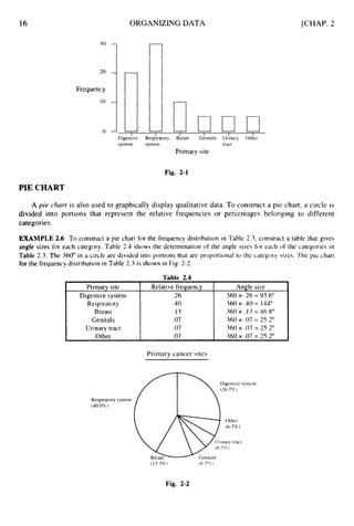
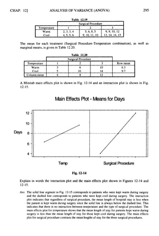
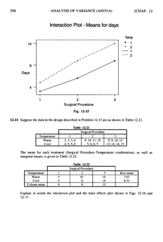
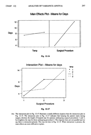
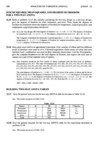
Downloaded 23 times


![CHAP. I] INTRODUCTION 7
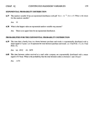
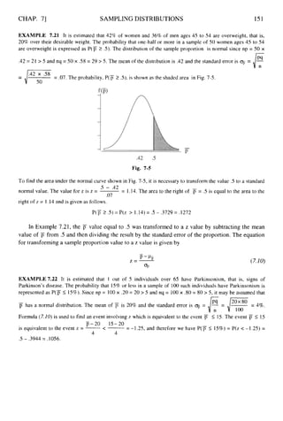
EXAMPLE 1.20 The following values were observed for the variables x and y: XI = I , x2 = 2, xj = 0, x4 = 4,
y1= 2, y2 = I , y3 = 4, and y4 = 5. The following computations show how the summation notation is used for two
variables.
ZXY
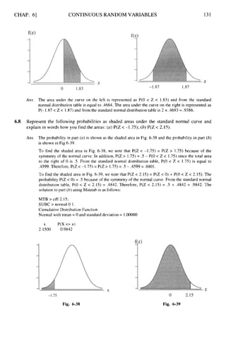
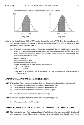
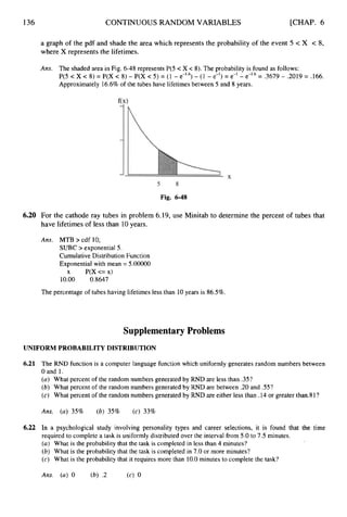
= xlyl + ~ 2 ~ 2
+xjyj + ~ 4 ~ 4
= 1 x 2 + 2 x 1 +0 x 4 +4 x 5 = 24
(Cx)(Cy)=(x1 +X2+Xj+Xq)(Y1 + y 2 + y 3 + y 4 ) = ( 1 + 2 + 0 + 4 ) ( 2 + 1 + 4 + 5 ) = 7 x 12=84
( C X ~ - ( C X ) ~ / ~ ) X ( Z ~ ~ - ( C Y ) ~ / ~ ) = ( ~
+ 4 + 0 + 1 6 - 7 2 / 4 ) ~ ( 4 +
1 + 16+25- 12*/4)=(8.75)~(10)=
87.5
COMPUTERSAND STATISTICS
The techniques of descriptive and inferential statistics involve lengthy repetitive computations as
well as the construction of various graphical constructs. These computations and graphical
constructions have been simplified by the development of computer software. These computer
software programs are referred to as statistical sojhare packages, or simply statistical packages.
These statistical packages are large computer programs which perform the various computations and
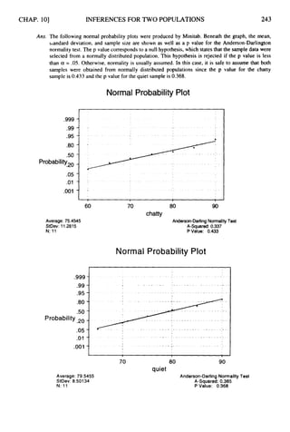
graphical constructions discussed in this outline plus many other ones beyond the scope of the
outline. Statistical packages are currently available for use on mainframes, minicomputers, and
microcomputers.
There are currently available numerous statistical packages. Four widely used statistical
packages are: MINITAB, BMDP, SPSS, and SAS. Many of the figures found in the following
chapters are MINITAB generated. MINITAB is a registered trademark of Minitab, Inc., 3081
Enterprise Drive, State College, PA 16801. Phone: 814-238-3280; fax: 8 14-238-4383; telex: 88 1612.
The author would like to thank Minitab Inc. for their permission to use output from MINITAB
throughout the outline.
Solved Problems
DESCRIPTIVE STATISTICSAND INFERENTIAL STATISTICS:
POPULATIONAND SAMPLE
1.1 Classify each of the following as descriptive statistics or inferential statistics.
(a) The average points per game, percent of free throws made, average number of rebounds
per game, and average number of fouls per game as well as several other measures
for players in the NBA are computed.
(b) Ten percent of the boxes of cereal sampled by a quality technician are found to be under
the labeled weight. Based on this finding, the filling machine is adjusted to increase the
amount of fill.
(c) USA Today gives several pages of numerical quantities concerning stocks listed in AMEX,
NASDAQ, and NYSE as well as mutual funds listed in MUTUALS.
(d)Based on a study of 500 single parent households by a social researcher, a magazine
reports that 25% of all single parent households are headed by a high school dropout.
Ans. (a) The measurements given organize and summarize information concerning the players and is
therefore considered descriptive statistics.](https://image.slidesharecdn.com/schaumoutlinesofbeginningstatistics-221128031359-68ac468e/85/Schaum-Outlines-Of-Beginning-Statistics-pdf-16-320.jpg)
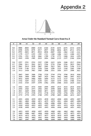
![CHAP. I] INTRODUCTION 13
Ans. interval or ratio
SUMMATION NOTATION
1.28 The following values are recorded for the variable x: x1 = 15, x2 = 25, x3 = 10, and x4 = 5. Evaluate the
following summations: Cx, Ex2, (CX)~,
and C(x - 5).
Ans. Ex = 55, Cx’ = 975, (CX)~
= 3025, C(x - 5) = 35
1.29 The following values are recorded for the variables x and y: xi =17, x2 = 28, x3 = 35, y1 = 20, y2 = 30,
and y3 = 40. Evaluate the following summations:Zxy, Cx2y2,and Cxy - ZxCy.
Ans. Cxy = 2580, Cx2y2= 2,781,200, CXY- CXCY= -4,620
1.30 Given that xI = 5, x2= 10, y1 = 20, and Cxy = 200, find y2.
Ans. y2 = 10](https://image.slidesharecdn.com/schaumoutlinesofbeginningstatistics-221128031359-68ac468e/85/Schaum-Outlines-Of-Beginning-Statistics-pdf-22-320.jpg)
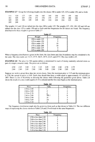
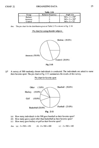

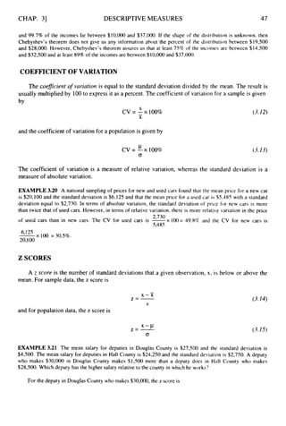
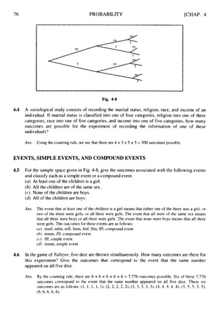
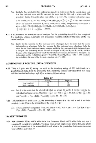
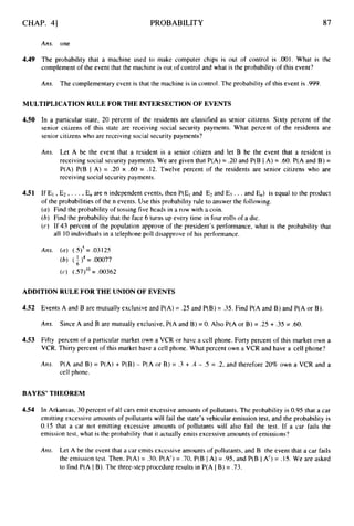
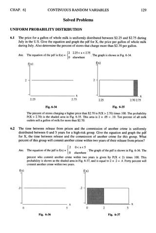
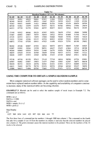
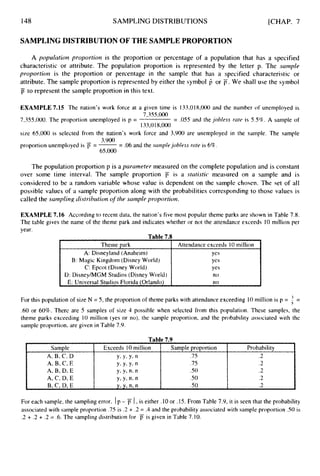
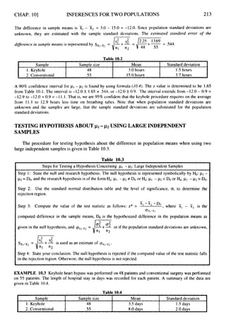
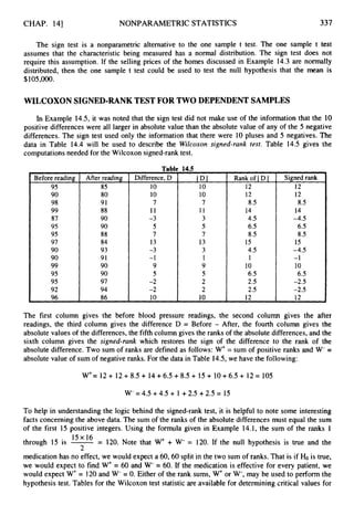
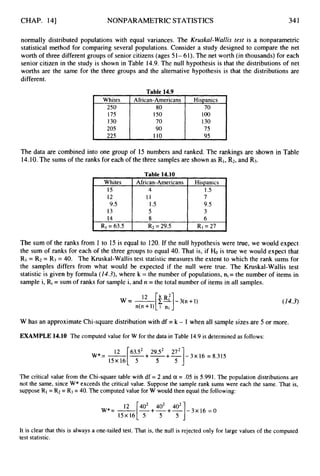
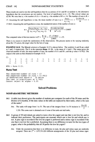
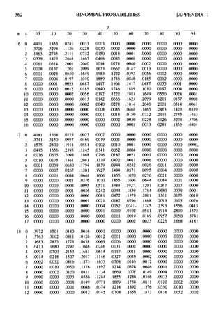
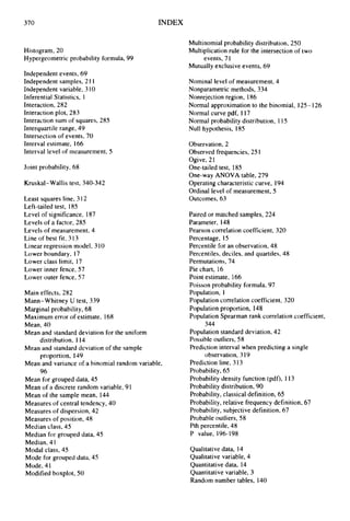
![64
1
2
Die2 3 -
4
5
6
PROBABILITY
J , 8 8 8 8 8
- 8 8 8 8 8 8
8 8 8 8 8 8
- 8 8 8 8 W W
-. 8 8 8 8 8
8 8 8 8 8
[CHAP. 4
first toss second toss outcome
HH
I
HT
TH
TT
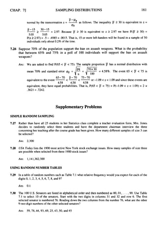
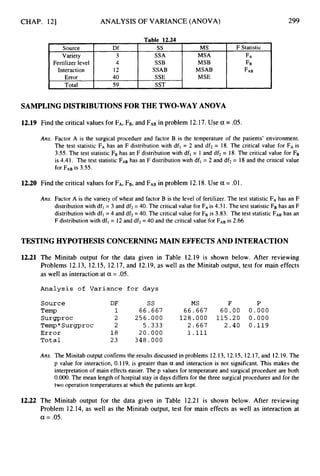
Fig. 4-1
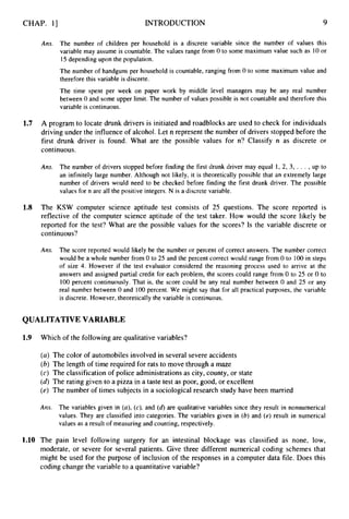
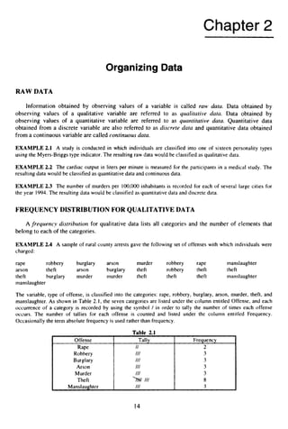
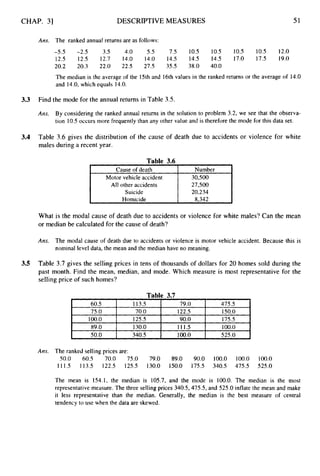
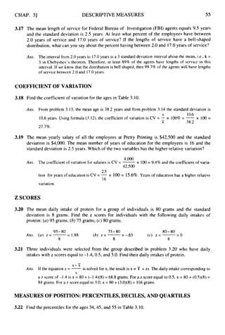
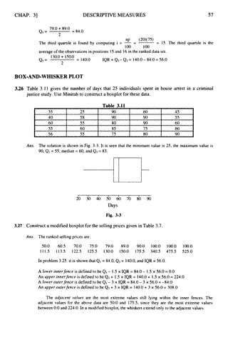
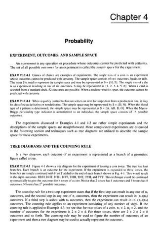
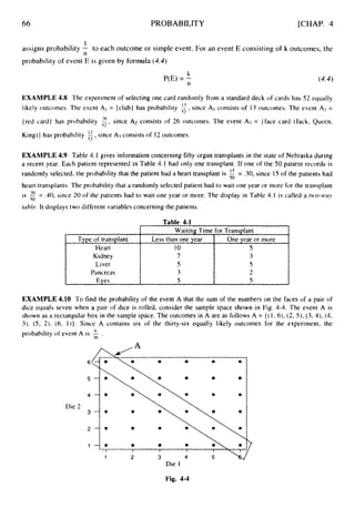
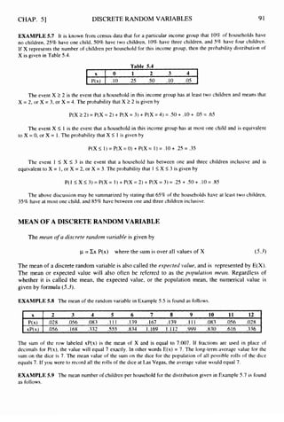
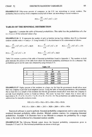
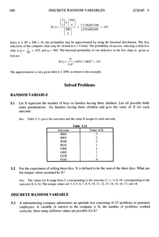
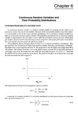
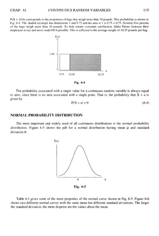
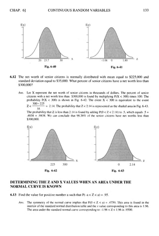
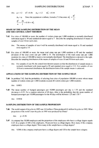
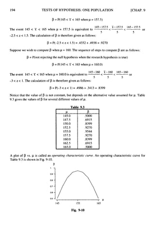
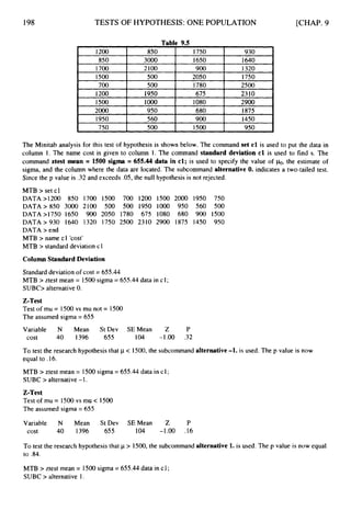
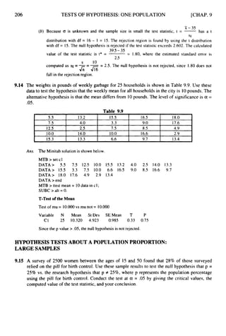
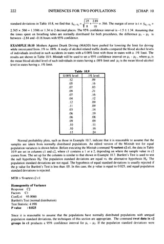
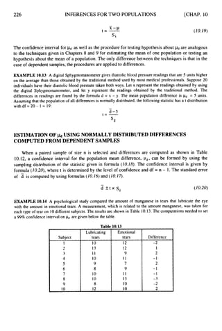
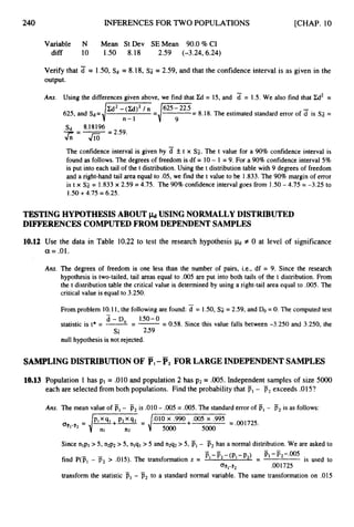
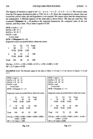
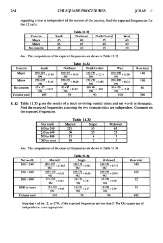
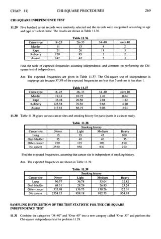
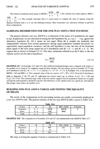
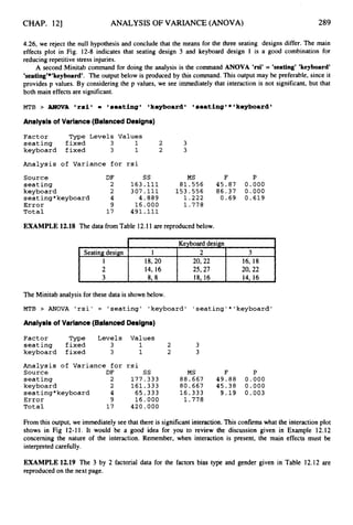
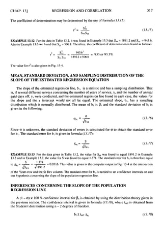
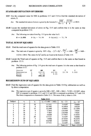
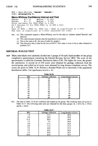
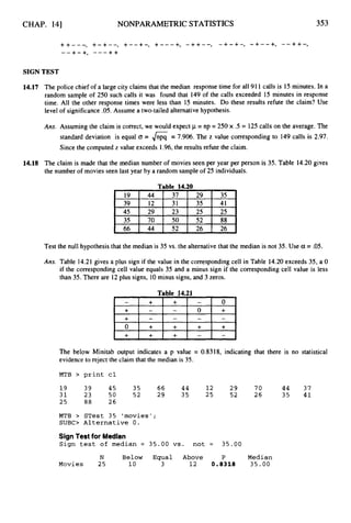
EXAMPLE 4.4 For the experiment of rolling a pair of dice, the first die may be any of six numbers and the
second die may be any one of six numbers. According to the counting rule, there are 6 x 6 = 36 outcomes. The
outcomes may be represented by a tree having 36 branches. The sample space may also be represented by a two-
dimensional plot as shown in Fig. 4-2.
Fig. 4-2
EXAMPLE 4.5 An experiment consists of observing the blood types for five randomly selected individuals.
Each of the five will have one of four blood types A, B, AB, or 0. Using the counting rule, we see that the
experiment has 4 x 4 x 4 x 4 x 4 = 1,024 possible outcomes. In this case constructing a tree diagram would be
difficult.
EVENTS, SIMPLEEVENTS, AND COMPOUNDEVENTS
An event is a subset of the sample space consisting of at least one outcome from the sample
space. If the event consists of exactly one outcome, it is called a simple event. If an event consists of
more than one outcome, it is called a compound event.
EXAMPLE4.6 A quality control technician selects two computer mother boards and classifies each as
defective or nondefective. The sample space may be represented as S = {NN, ND, DN, DO], where D
represents a defective unit and N represents a nondefective unit. Let A represent the event that neither unit is
defective and let B represent the event that at least one of the units is defective. A = { NN} is a simple event and
B = {ND,DN, DD) is a compound event. Figure 4-3 is a Venn Diagram representation of the sample space S](https://image.slidesharecdn.com/schaumoutlinesofbeginningstatistics-221128031359-68ac468e/85/Schaum-Outlines-Of-Beginning-Statistics-pdf-73-320.jpg)

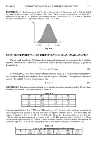
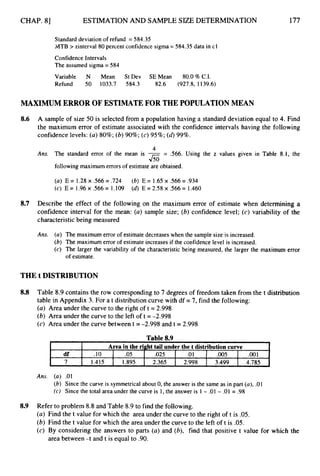
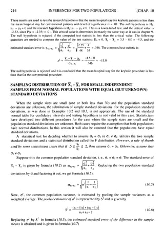
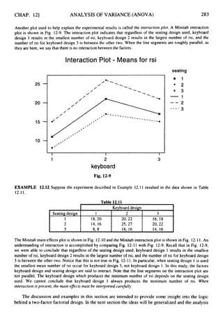
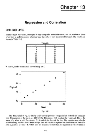
![CHAP. 81
2 .
1
ESTIMATION AND SAMPLE SIZE DETERMINATION 183
Fig. 8-5
CONFIDENCE INTERVAL FOR THE POPULATION PROPORTION:LARGE SAMPLES
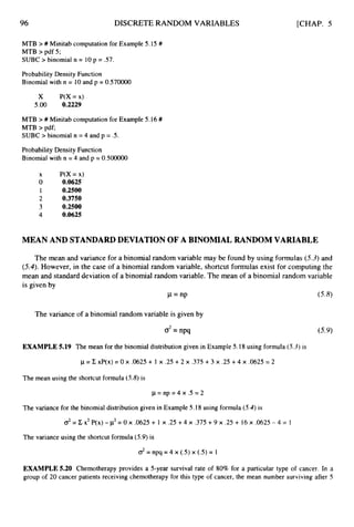
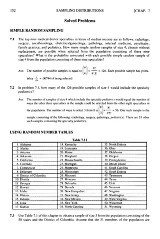
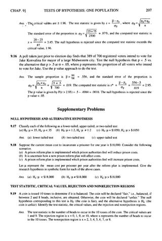
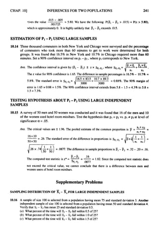
8.29 In a survey of 900 adults, 360 responded “yes” to the question “Have you attended a major league
baseball game in the last year?” Determine a 90% confidence interval for p, the proportion of all adults
who attended a major league baseball game in the last year.
Am. The sample proportion attending a game in the last year is iT = .40 and the proportion not
attending is = .60. The z value for a 90% confidence interval is 1.65. The confidence interval
for p is p- z
]
y< p < p+ ZJF.
The maximum error of estimate is E = z,/?= .027. The
lower limit of the confidence interval is .40 - .027 = .373 and the upper limit is .40 +.027 = .427.
The 90%interval is (.373, .427).
8.30 Use the data in Table 8.8, found in problem 8.4, to find a 99% confidence interval for the proportion of
all taxpayers receiving a refund who receive a refund of more than $500.
Am. Thirty-seven of the fifty refunds in Table 8.8 exceed $500.The sample proportion exceeding $500
is .74. The z value for a 99% confidence interval is 2.58. The confidence interval for D is
p- z/F-
< p < p+ z/F-.
The maximum error of estimate is E = z,/?= .16 The lower
limit is .74 - .16 = .58 and the upper limit is .74 + .16 = .90.The 99%interval is ( 5 8 , .90).
DETERMINING THE SAMPLE SIZE FOR THE ESTIMATIONOF THE POPULATION MEAN
8.31
8
.
3
2
The estimated standard deviation of commutingdistances for workers in a large city is determined to be 3
miles in a pilot study. How large a sample is needed to estimate the mean commuting distance of all
workers in the city to within .5 mile with 95% confidence?
. For this problem, E = .5, z = 1.96, and CT is estimated to be
Am. The sample size is given by n = -
3. The sample size is determined to be 139.
Z2 o2
E2
In problem 8.31, what size sample is required to estimate p to within .I mile with 95% confidence?
Am. n = 3,458](https://image.slidesharecdn.com/schaumoutlinesofbeginningstatistics-221128031359-68ac468e/85/Schaum-Outlines-Of-Beginning-Statistics-pdf-192-320.jpg)
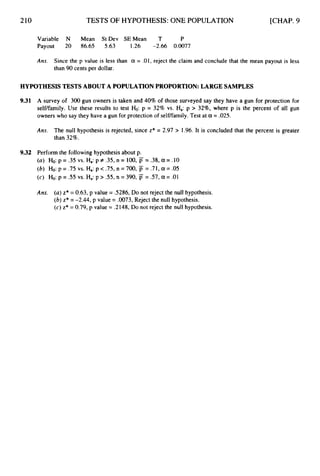
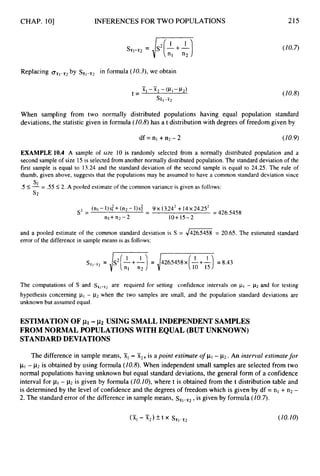

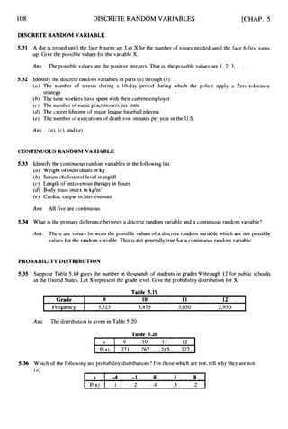
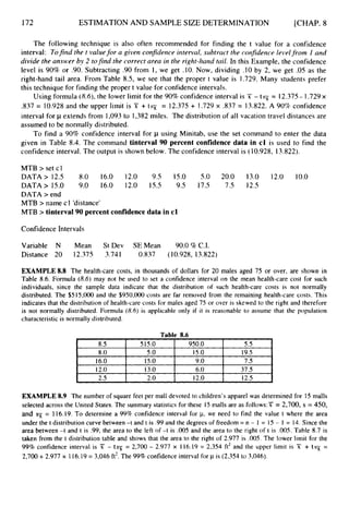
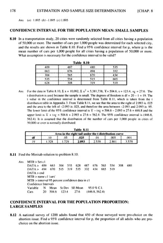
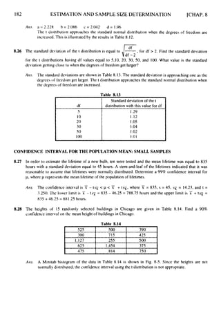
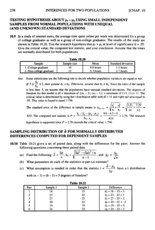
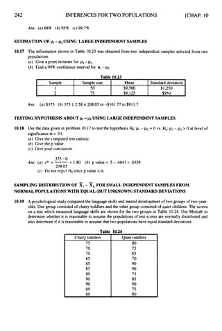
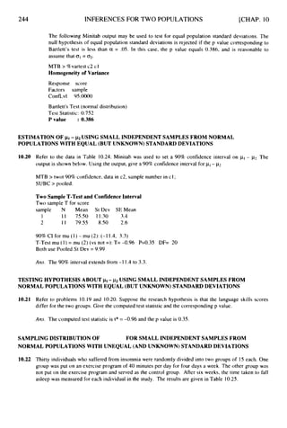
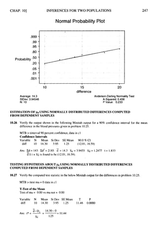
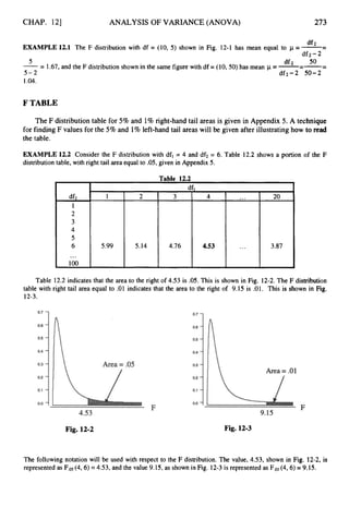
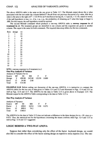
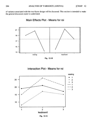
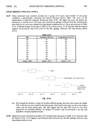
![236 INFERENCES FOR TWO POPULATIONS [CHAP. 10
Table 10.19
I
Omaha
75
70
70
65
85
85
80
90
90
60
60
Kansas City
80
75
75
85
85
100
60
65
95
105
70
MTB > twot 99% confidence data in c2, groups in c 1;
SUBC > pooled.
Two SampleT-Testand ConfidenceInterval
Two sample T for rate
city N Mean St Dev SEMean
1 1 1 75.5 11.3 3.4
2 11 81.4 14.3 4.3
99%CI for mu (1) - mu (2): (-2 1.6, 9.7)
T-Test mu (1) = mu (2) (vs not =):T =-1.07 P = 0.30 DF = 20
Both use Pooled St Dev = 12.9
-
Ans. The difference in sample mean is '51, - x2 = 75.5 - 81.4 =-5.9.
(nl -1)s: +(n2 - I) s! 10x 127.69+10x204.49
= 166.09,and S =
-
-
The pooled variance is S2 =
nl+ n2 -2 11+11-2
4166.09 = 12.9.
The standard error of the difference in the sample means is SxI-x2 = &
2
[
;
+
;
] =
1
7
3
166.09~-+- ~ 5 . 5 0 .
Using the t distributiontable with df = 20 and right-hand tail area equal to .005, we find the t value
is 2.845. The 99% margin of error is 2.845 x 5.50 = 15.6. The 99% confidence interval extends
from -5.9 - 15.6= -21.5 to -5.9 + 15.6= 9.7.
TESTING HYPOTHESIS ABOUT ~ 1 -
~2 USING SMALL INDEPENDENT
SAMPLES FROM NORMAL POPULATIONS WITH EQUAL (BUT UNKNOWN)
STANDARD DEVIATIONS
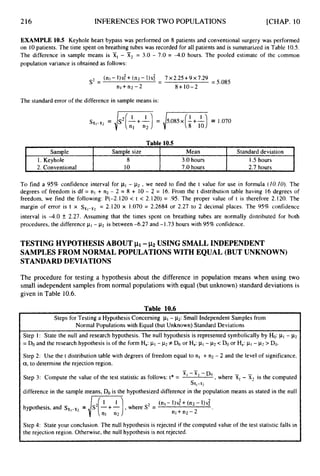
10.6 Use the motel rate data in Table 10.I9 and the Minitab output given in problem 10.5 to test the
null hypothesis Ho:pI- p2 = 0 vs. Ha:pl -p
2 # 0 at significance level a = .O 1.
(a) Give the critical values for performingthe test.
(b) Give the computed value of the test statistic, and your conclusion based upon this value
and the critical value in part (a).
(c) Give the p value and your conclusion based on this value.](https://image.slidesharecdn.com/schaumoutlinesofbeginningstatistics-221128031359-68ac468e/85/Schaum-Outlines-Of-Beginning-Statistics-pdf-245-320.jpg)
![CHAP. 101
Ans. (a)
INFERENCES FOR TWO POPULATIONS 237
The degrees of freedom for the t distribution is 20. Since the research hypothesis is two-tailed,
the significance level is divided by 2 and .005 is put into each tail of the distribution. By
consulting the t distribution table, we find that for df = 20 and right-tail area = .005, the t
value is 2.845. The critical values are k2.845.
The computed t value, from the Minitab output in problem 10.5,is t* = -1.07. Since this value
does not fall in the rejection region, the null hypothesis is not rejected. It cannot be concluded
that the mean motel rates differ for the two cities.
The p value, from the Minitab output in problem 10.5,is equal to 0.30. Since this exceeds the
preset level of significance,the null hypothesis is not rejected. The same conclusion is reached
as in part (b).
SAMPLING DISTRIBUTION OF Xi-X,FOR SMALL INDEPENDENT
SAMPLES FROM NORMAL POPULATIONS WITH UNEQUAL
(AND UNKNOWN) STANDARD DEVIATIONS
10.7 Refer to problem 10.4.Suppose the two populations have unequal population variances. What
changes are needed to the answers given in the problem?
Am. Since the population variances are unequal, the sample variances are not pooled together to
estimate a common population variance. The standard error of the difference in the sample means
- -
X i - X 2 4 - 5
is given by sxl-siz has a t distribution and
sx,-iT2
the degrees of freedom is given by df = minimum of { (nl - l), (n2- 1)) = minimum of { 9, 14) =
9. Note that the degrees of freedom is reduced from 23 to 9. This problem illustrates the
importance of checking the assumptions underlying the estimation and testing procedures. The
computation of the test statistic as well as the degrees of freedom is determined by the assumption
concerning the variances of the two populations.
ESTIMATION OF 1 1 -~2 USING SMALL INDEPENDENT SAMPLES
FROM NORMAL POPULATIONS WITH UNEQUAL (ANDUNKNOWN)
STANDARD DEVIATIONS
10.8 Refer to problem 10.5. Compute the standard error of the difference in means, the degrees of
freedom, and the 99% confidence interval assuming unequal population variances. Compare
the results with those in problem 10.5.
Ans. The standard error of the difference in sample means isSsr,-n2= +-
nl n2 I 1 11
which equals 5.50. This is the same answer obtained in the equal variances case. This will always
occur if the sample sizes are equal.
The degrees of freedom is df = minimum of ( ( n l - I), (n2 - l)] = minimum of { 10, 10) = 10.
Using the t distribution table with df = 10and right-hand tail area equal to .005, we find the t value
is 3.169. The 99% margin of error is 3.169 x 5.50 = 17.4. The 99% confidence interval extends
from -5.9 - 17.4= -23.3 to -5.9 + 17.4 = 11.5.
The 99% confidence interval in the equal variances case is (-21.5, 9.7). The 99% confidence
interval for the unequal variances case is (-23.3, 11.5). Note that the interval in the unequal
variances case is wider.](https://image.slidesharecdn.com/schaumoutlinesofbeginningstatistics-221128031359-68ac468e/85/Schaum-Outlines-Of-Beginning-Statistics-pdf-246-320.jpg)
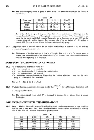
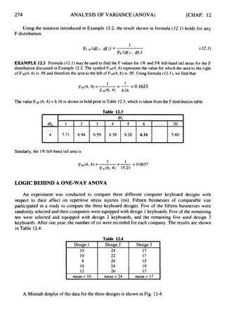
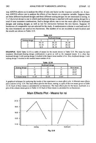
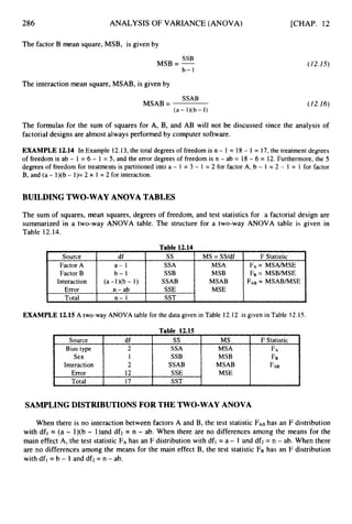
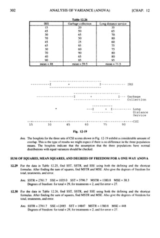
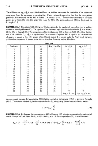
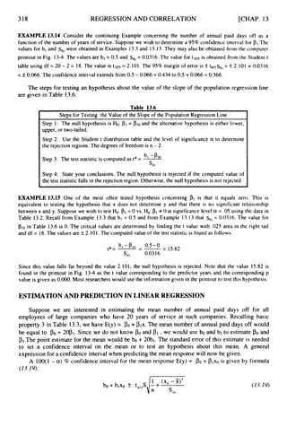
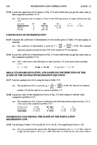
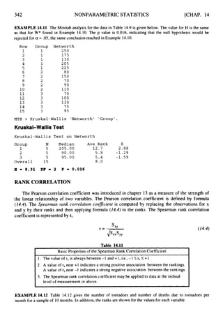
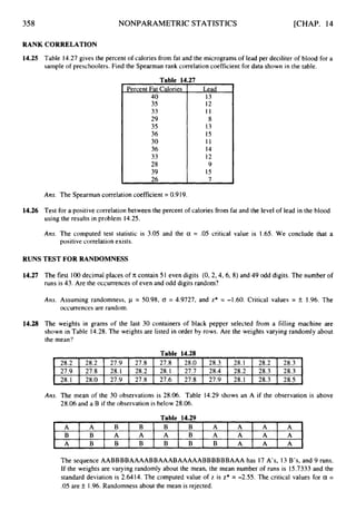
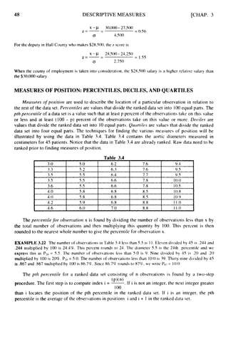
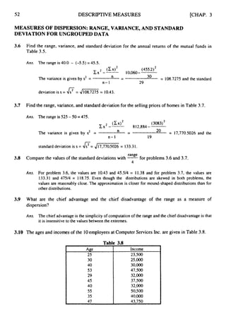
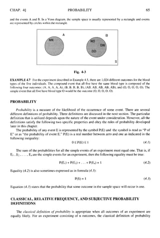
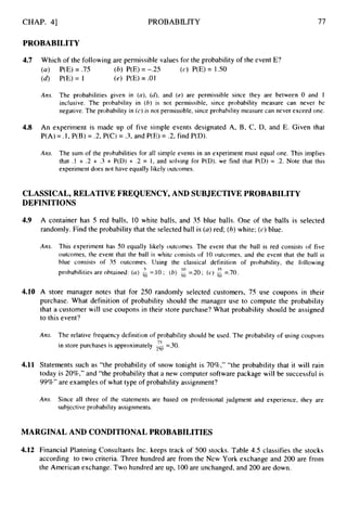
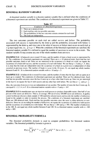
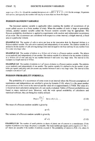
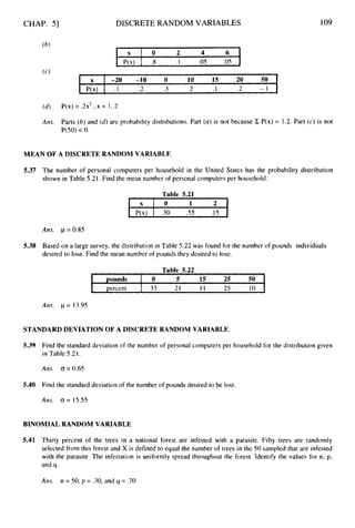
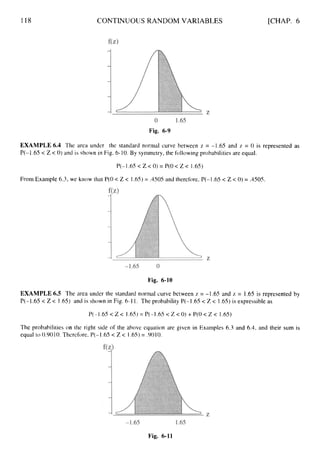
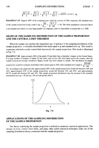
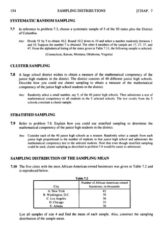
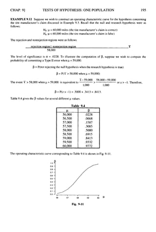
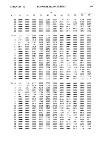
![APPENDIX I] BINOMIALPROBABILITIES 361
P
n x .05 .lO .20 30 .40 S O .60 .70 .80 .90 .95
1
0
11
12
.oooo
.OOoo
.oooo
.m
.oooo
.oooo
.m
.oOOo
.m
.o002
.m
.OoOo
.0025 .
0
1
6
1
.OOo3 .0029
.oooo .OOo2
.0639
.O174
.0022
.1678
.07
12
.0138
.2835
.2062
.0687
.2301
.3766
.2824
.0988
.34
13
5404
.5 133
.35
12
.
1
1
0
9
.02
1
4
.0028
.OOo3
.m
.m
.moo
.m
.0000
.GO00
.oOOo
.m
.2542
.3672
.2448
.0997
.0277
,0055
.OOo8
*OOo1
.m
.OOoO
.oOOo
,0000
.oooo
.OOoo
.0550
.1787
.2680
.2457
.1535
.069
1
.0230
.0058
.0011
.0001
.oo00
.oOOo
.m
.m
.
0
0
9
7
.0540
.1388
.2181
.2337
.1803
.1030
.0442
.0142
.0034
.o
00
6
.o001
.oooo
.m
.0013 .
o
0
0
1
.0113 .
0
0
1
6
.0453 .0095
.1107 .0349
.I845 .0873
.2214 .1571
.1968 .2095
.1312 .2095
.0656 .1571
.0243 ,0873
.0065 .0349
.0012 .0095
.OOo1 .0016
.m .
o
0
0
1
.m
.ooo1
.0012
.0065
.0243
.0656
,1312
.I968
.2214
,1845
.1107
.0453
.0113
,0013
.oOOo
.OOoo
.OOo1
.OOo6
.0034
.0142
0442
.I030
.1803
.2337
.2181
.1388
.0540
.0097
.m
.m
.m
.m
.
o
0
0
1
.0011
.0058
.0230
.
0
6
9
1
.1535
.2457
.2680
.1787
.0550
.m
.oooo
.m
.m
.m
.m
.OOo1
.OOo8
.0055
.0277
.0997
.2448
.3672
.2542
.OoOo
.OoOo
.0000
.m
.m
.m
.m
.m
.0003
.0028
.02
1
4
. I 1
0
9
.35
12
.5 133
13 0
1
2
3
4
5
6
7
8
9
1
0
11
12
13
1
4 0
1
2
3
4
5
6
7
8
9
10
11
12
13
1
4
.4877
.3593
.I229
.0259
.0037
.o004
.m
.oooo
.OOoO
.oooo
.m
.m
.m
.moo
.OOoO
,2288
.3559
,2570
.1142
.0349
.0078
.OO13
.OOo2
.m
.moo
.0000
.OOoo
.m
.oOOo
.0000
.0440
.1539
.2501
.2501
.1720
.0860
.0322
.#92
.0020
.oO03
.m
.OoOo
.OoOo
.oooo
.0000
.0068
.0
40
7
.1134
.1943
.2290
.1963
.1262
.
0
6
18
.0232
.0066
.
0
0
1
4
.o002
.m
.oooo
.o000
.OOo8 .
o
0
0
1
,0073 .
0
0
0
9
.0317 .0056
.0845 .0222
.1549 .
0
6
1
1
.2066 .1222
.2066 .1833
.1574 .2095
.0918 .1833
.MO8 .1222
.0136 .
0
6
1
1
.0033 .0222
.OOo5 .0056
.oO01 ,0009
.moo .o001
.0000
.OOO1
.OOo5
.oo33
.0136
9408
.
0
9
18
* 1574
.2066
.2066
.1549
.0845
.03
17
.073
.WO8
.m
.m
.OOoO
.OOo2
.OO 1
4
.
0
0
6
6
.0232
.06
I8
.1262
.1963
.2290
.1943
.I134
.MO7
.0068
.oooo
.OOOo
.moo
.m
.0000
.o003
.oo20
.0092
.0322
.0860
.1720
.2501
.2501
.1539
.0440
.0000
.moo
.m
.moo
.oooo
.m
.m
.OOo2
.0013
.0078
.0349
.1142
.2570
.3559
.2288
.OoOo
.m
.m
.m
.oOOo
.m
.moo
.m
.oOOo
.0004
.0037
.0259
.1229
.3593
.4877
1
5 0
1
2
3
4
5
6
7
8
9
1
0
11
12
13
1
4
15
.4633
.3658
.1348
.0307
.
0
0
4
9
.OOo6
.oOOo
‘.0000
.moo
.oooo
.oooo
.m
.moo
.oooo
.m
.oooo
.2059
.3432
.2669
.1285
.0428
.O105
.0019
.o003
.m
.oooo
.oooo
.0000
.0000
.oooo
.moo
.m
.0352
.1319
.2309
.250
1
.1876
.1032
.0430
.0138
.0035
.
0
0
0
7
.ooo1
.m
.m
.oooo
.OoOo
.oooo
. w 7
.0305
.
0
9
1
6
.1700
.2
186
.206
1
.1472
.0811
.0348
,0116
.0030
.
0
0
0
6
.OOo1
.oooo
.0000
.m
.0005 .OOOO
.0047 .0005
.0219 .0032
.0634 .0139
.1268 .0417
.1859 .
0
9
1
6
.2066 .1527
.1771 .1964
.1181 .I964
.0612 .I527
.0245 .
0
9
1
6
-0074 .
0
4
1
7
.0016 .0139
.0003 .0032
.0000 .WO5
.m .oOOo
.OOoo
.0000
.0003
.0016
.0074
.0245
.
0
6
12
.1181
.1771
.2066
.1859
.I268
.0634
.02
1
9
.0047
.OOo5
.m
.m
.m
.OOo1
.m
.0030
.0116
.0348
.OS1 1
.1472
.206
1
.2
186
.1700
.
0
9
1
6
.0305
.0047
.m
.m
.oOOo
.m
.oOOo
.0001
.WO7
.oo35
.0138
0430
.1032
.1876
.250
1
.2309
.1319
.0352
.OOoo
.oooo
.m
.0000
.m
.oOOo
.moo
.oo00
.o003
.0019
.O105
.0428
-1285
.2669
.3432
.2059
.m
.m
.moo
.moo
.oOOo
.oooo
.m
.m
.oOoO
.0000
.w06
.0049
.0307
.1348
.3658
.4633](https://image.slidesharecdn.com/schaumoutlinesofbeginningstatistics-221128031359-68ac468e/85/Schaum-Outlines-Of-Beginning-Statistics-pdf-370-320.jpg)

This document provides an introduction to statistics, including descriptive and inferential statistics. Descriptive statistics involves organizing and summarizing data using graphs, charts, tables, and statistical measures. Inferential statistics allows conclusions to be drawn about an entire population based on a sample of that population. A population is the complete set of data being studied, while a sample is a subset of the population. Examples are given to illustrate key concepts like populations, samples, descriptive versus inferential statistics, and how statistics are used in areas like polling and crime reporting.


![[Sundstrom_Ted.]_Mathematical_Reasoning_Writing - Copy.pdf](https://cdn.slidesharecdn.com/ss_thumbnails/sundstromted-221124155318-3b41c59e-thumbnail.jpg?width=640&height=640&fit=bounds)


