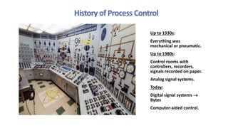
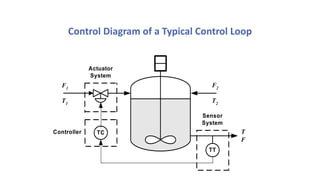
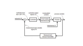
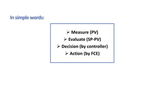
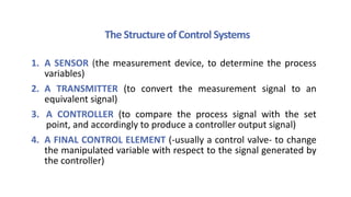
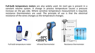
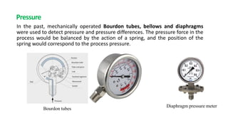
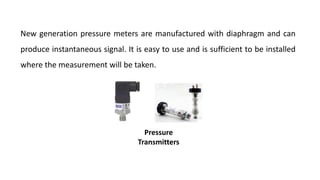
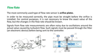
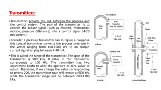
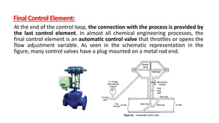
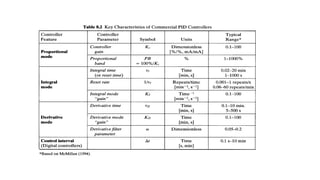
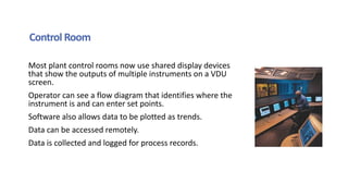
KMM4631
PROCESS DYNAMICS
AND CONTROL
Prof. Dr. Elçin YILMAZ & Assist. Prof. Dr. Ekin KIPÇAK
2024-2025 Fall
CONTROL INSTRUMENTS
&
CONTROLLERS
History of Process Control
Up to 1930s:
Everything was
mechanical or pneumatic.
Up to 1980s:
Control rooms with
controllers, recorders,
signals recorded on paper.
Analog signal systems.
Today:
Digital signal systems 
Bytes
Computer-aided control.
Today
Computers are used to monitor the condition of the process.
Signals and the status of the process are monitored on the
computer screen.
Many signals are still transmitted in analog electronic form, but
the use of digital buses and networks is increasing day by day. These
systems provide much more calculation capability and enable on-
line operation (while the process is running) based on the
mathematical model of the process.
Despite all these changes, the basis of control system structures
and control algorithms is the same as 30 years ago.
Signals:
Analog: Air pressure signal (3-15 psig)
Current signal (4-20 mA)
Voltage signal (0-10 V)
For instance, pneumatic valves convert signals between 4-20 mA
to signals between 3-15 psig.
Digital: Bytes
As discussed earlier, the feedback control loop includes:
 A sensor to detect process variables;
 A transmitter to convert the measurement signal to an equivalent
signal (an air pressure signal in pneumatic systems or a current signal in
analog electronic systems),
 A controller that compares the process signal with a desired set point
and generates a suitable controller output signal, and
 Adjusting according to the signal generated by the controller, It
consists of a final control element that modifies the variable. Usually
the last control element is an air operated control valve that opens and
closes to change the flow rate of the set current.
The figure shows a diagram of a process controlled by feedback control.
•Sensor, transmitter and control valve are physically located on the
process (in operation).
•The controller is usually in a remote control room, on a panel or on a
computer.
•The current signal transfer from the transmitter to the controller and
from the controller to the final control element or the connection
between the units is provided by cables.
•Control parts used in chemical and petroleum plants are analog or
digital.
•Analog signals use an air pressure signal (3 to 15 psig) or a current /
voltage signal (4-20 mA or 0-10 V DC).
•The parts are powered by 1.4 bar air pressure or 24 V DC electricity.
•Pneumatic systems send air pressure through small pipes. Analog
electronic systems use cables. Because many valves still operate with air
pressure, flow signals are often converted into air pressure.
•An "I / P" (current to pressure) converter is used to convert signals
between 4-20 mA into signals of 3-15 psig.
•There is a manual / automatic on-off assembly (or software) in the
control room. When starting up or in abnormal situations, the plant
operator or engineer may want to adjust the control valve instead of the
controller. The power button is usually on the control panel or computer.
In the "manual" position, the operator or engineer can adjust the valve
as desired. In the automatic position, the valve is adjusted directly by
controlling correction commands.
Eachcontrollermustdothefollowing:
a) It should determine the value of the control variable,
(the signal from the transmitter) (CV or PV)
b) Determine the set value signal, (SP or SV)
c) Determine the value of the signal to be sent to the
valve, (Controller output) (CO)
d) Have Manual / Automatic buttons,
e) It should have a button to enter the set value while
the controller is automatic,
f) When the controller is in manual, there should be a
button to send a signal to the valve.
Control Instruments
Control Diagram of a Typical Control Loop
Controller
F1
T1
T
F
F2
T2
TC
Actuator
System
TT
Sensor
System
In simplewords:
 Measure (PV)
 Evaluate (SP-PV)
 Decision (by controller)
 Action (by FCE)
The Structure of Control Systems
1. A SENSOR (the measurement device, to determine the process
variables)
2. A TRANSMITTER (to convert the measurement signal to an
equivalent signal)
3. A CONTROLLER (to compare the process signal with the set
point, and accordingly to produce a controller output signal)
4. A FINAL CONTROL ELEMENT (-usually a control valve- to change
the manipulated variable with respect to the signal generated by
the controller)
Controller
The controller is a device, which monitors and affects the operational
condition of a dynamic system. In a process control system the controller
is not necessarily limited to one variable, but can measure and control
many variables.
Measuring element
In order to make the controlled variable accessible to the controller, it
must be measured by a measuring element or primary sensing element
(sensor, transducer) and converted from a physical variable to an
electrical signal that can be processed by the controller as an input.
The control loop starts with the measurement. An assembly has been
developed to measure many variables online. The most important
variables in chemical engineering processes; flow rate, temperature,
pressure and level. There are also measurement tools to measure
variables such as pH, density, viscosity, infrared and ultraviolet
absorption, and refractive index.
If the measuring instrument used measures the change in the variable
with a delay, the dynamic model of that measuring instrument or the
transfer function must be removed. If measurement is taking place
without delay, the transfer function of the meter will only equal the gain
value.
Sensors:
It is a device that can detect physical variables, such as temperature, light
intensity, or motion, and have the ability to give a measurable output
that varies in relation to the amplitude of the physical variable.
 Temperature sensors
 Flow rate sensors
 Level sensors
 Pressure sensors
 Composition analyzers
Temperature
Thermocouples consist of two wire legs made from different metals.
The wires legs are welded together at one end, creating a junction. This
junction is where the temperature is measured.
There are many types of thermocouples, each with its own unique
characteristics in terms of temperature range, durability, vibration
resistance, chemical resistance, and application compatibility.
Type J, K, T, & E are “Base Metal” thermocouples, the most common
types of thermocouples.
Type R, S, and B thermocouples are “Noble Metal” thermocouples,
which are used in high temperature applications
In the table, thermocouples made of various metal and metal alloys, the measuring
range and the mV electrical signal generated per unit °C are given. The control engineer
should choose a thermocouple according to the temperature range to be measured.
The dynamic response of many sensors is generally much faster than the
dynamic behavior of the process itself. The time constant of a temperature
gauge and a thick thermocouple housing can be 30 seconds or more.
Thermocouples are produced with metal sheaths made of various alloys
according to the corrosive conditions, mechanical wear, chemical and physical
abrasive properties of the process in which they will be used. Thermocouples
to be used at extremely high temperatures are covered with porous or non-
porous ceramic sheaths against thermal shocks. If the thermocouple is
covered with polymer or other material, the response time may take several
minutes. Since this situation affects the control performance, the dynamic
model of the thermocouple should be created and included in the control
loop dynamics.
 
16 90
1 1
s
s
s s
K mA C
G s
s s
 

 
 
Full-bulb temperature meters are also widely used. An inert gas is present in a
constant volume system. A change in process temperature causes a pressure
increase on the gas side. Where sensitive temperature measurement is required,
resistance thermometers are used. The principle of use is that the electrical
resistance of the wires changes as the temperature changes.
Full-bulb temperature meter Infrared thermometer Resistance thermometer
Pressure
In the past, mechanically operated Bourdon tubes, bellows and diaphragms
were used to detect pressure and pressure differences. The pressure force in the
process would be balanced by the action of a spring, and the position of the
spring would correspond to the process pressure.
Bourdon tubes
Diaphragm pressure meter
New generation pressure meters are manufactured with diaphragm and can
produce instantaneous signal. It is easy to use and is sufficient to be installed
where the measurement will be taken.
Pressure
Transmitters
Flow Rate
The most commonly used type of flow rate sensor is orifice plates.
In order to be measured correctly, the pipe must be straight before the orifice is
installed. For control purposes, it is not necessary to know the exact value of the
flow, but the changes in the flow rate should be known.
Signals from flow rate measurements are often noisy due to oscillations around the
actual value caused by turbulent flow. Such signals must be passed through the filter
(an electronic device) before being sent to the controller.
Turbine meters are also
widely used. They are very
expensive, but provide a more
accurate flow measurement.
Other types of flowmeters include sonic flowmeters, magnetic flowmeters, rotameters,
and pitot tubes.
Sonic flowmeters
Magnetic flowmeters
Rotameter
Pitot tubes
Fluid Level
It is possible to measure the fluid level in many ways. In principle, it is possible to
measure the liquid level in three different ways:
1. Tracking the swimming position of an object lighter than the fluid (Buoy/Float),
2. Measuring the apparent weight of a heavy cylinder,
3. Measuring instruments based on the measurement of the hydrostatic pressure of
the liquid level have been developed.
Float level meter
Ultrasonic level meter
Hydrostatic
level meter
Composition Measurement
Some components can be detected at low concentrations using sensors that have been
designed to pick up that component.
Examples: O2, CO, H2S, H2
Component sensors are often sensitive to other components, so check carefully with
vendor to make sure the device is rated for the application.
More detailed composition can be measured by on-line GC methods.
TCD: thermal conductivity detector
FID: flame ionization detector
Response can be slow (5 to 30 minutes), particularly if a long column is used.
Online NIR can be used in some cases.
Composition is often inferred from other properties.
Boiling point
Conductivity
pH and Conductivity Meter Density and Viscosity Meter
Portable Gas Chromatograph for
gas composition measurement
Chapter
9
Languageproblem
Synchronization between sensor and controller, controller and FCE etc.
FCE should understand what Controller speaks
We need a translator (I/P, I/V, P/I)
Chapter
9
Transmitters:
•Transmitters provide the link between the process and
the control system. The goal of the transmitter is to
convert the sensor signal (such as millivolt, mechanical
motion, pressure difference) into a control signal (4-20
mA current).
•Consider a pressure transmitter like in Figure a. Suppose
this special transmitter converts the process pressure in
the vessel ranging from 100-1000 kPa to an output
current signal varying between 4-20 mA.
•This is called the range of the transmitter. The span of the
transmitter is 900 kPa. 0 value in the transmitter
corresponds to 100 kPa. The transmitter has two
adjustment knobs to alter the aperture or zero value to
adjust. Therefore, if we change the value corresponding
to zero to 200, the transmitter span will remain at 900 kPa
while the transmitter range will be between 200-1100
kPa.
The dynamic response of many transmitters is generally faster than that of process
and control valves. As a result, we can think that the transfer function of the
transmitter is only equal to the gain value (a step change entering the transmitter
suddenly comes out as a step function at the output). The gain of such a pressure
transmitter would be as follows;
Hence, the transmitter is simply a converter that converts process variables into an
equivalent signal.
Figure b shows a temperature transmitter that receives the thermocouple input
signal and converts the process temperature ranging from 10-100°C to a current
signal of 4-20 mA.
The temperature transmitter has a range of 10-100°C, a span of 90°C and a zero
value of 10°C. The temperature transmitter gain is as follows;
 
20 mA 4 mA 16 mA
1000 kPa 100 kPa 900 kPa
T T
G s K

  

 
20 mA 4 mA 16 mA
100 C 10 C 90 C
s s
G s K

  
   
 
16 90
1 1
s
s
s s
K mA C
G s
s s
 

 
 
Instrument Selection Criteria
•Solid/gas/liquid, corrosive fluid
•Nature of signal, speed of response
•Accuracy, measurement range
•Costs
•Previous plant practice
•Available space
•Maintenance, reliability
•Materials of construction
•Invasive/non-invasive
•Environmental/safety (enclosures, fugitive emissions)
Final Control Element:
At the end of the control loop, the connection with the process is provided by
the last control element. In almost all chemical engineering processes, the
final control element is an automatic control valve that throttles or opens the
flow adjustment variable. As seen in the schematic representation in the
figure, many control valves have a plug mounted on a metal rod end.
When the metal rod moves up and down, the plug opens and closes the
orifice opening. It is mounted on a diaphragm that moves with the
change of air pressure acting on the plug.
Air pressure (pneumatic signal) is provided by the IP converter that
converts the mA current from the controller into a pneumatic signal (3-
15 psig). These converters function with an external supply of 20 psig
(1.4 bar). Air pressure force is countered by a spring. Valves are designed
not to be in a fully open or fully closed position. The action for process
safety corresponds to the influence of the setting variable. For example,
if the valve is adjusting steam or fuel, we want the flow to be cut off
completely. If the valve adjusts the cooling water to a reactor, we want
the flow to be maximized immediately.
Actuator or solenoid valves are used when the flow rate is low.
Actuators are electric or air pressure operated and sliding. They open or
close the valve to the desired extent according to the incoming air
pressure or analog signal (current).
Solenoid valves operate directly with 220 V electricity, and the way they
work is completely magnetic. They are used in conjunction with an
electrical relay to which the cables from the controller are connected.
They usually work with a contact (on-off) output signal, and the valve is
completely open when the signal arrives, completely closed when the
signal is disconnected. Control or setting change is achieved by setting
the stay times on or off. They are generally preferred in systems where a
simple control will be performed.
Solenoid valve
Actuator Current-pneumatic
(IP) converter
Controllers
1.On Off Controllers
2.Proportional Controllers (P)
3.Proportional Integral Controllers (PI)
4.Proportional Derivative Controllers (PD)
5.Proportional Integral Derivative Controllers (PID)
On Off Controllers:
The manipulated variable is completely shut down or completely
opened when the value of the controlled variable is higher or smaller
than the set point value, respectively.
It operates completely mechanically and is preferred in simple systems,
where precise control is not required.
Household irons, water heaters, electric ovens, aquarium heaters, old-
style refrigerators, air compressors, hydrophores are controlled in this
way.
System never reaches steady-state.
A hysteresis band occurs during this oscillation.
The manipulated variable is closed when the controlled variable reaches
the top level and the manipulated variable is opened when the control
variable is at the bottom level.
It is the type of controller where the
controller output is directly
proportional to the error. Its
mathematical expression and Laplace
form are given by the following
expression;
The bias signal is a constant and the
controller output value in the absence
of any deviation. Kc is called the
controller gain. When the gain is large,
the controller output will be larger for a
given deviation. For example, if the gain
is 1, for a deviation of 10% of the full
scale, the controller output will change
by 10% of the scale. Often times the
term proportional band (PB) is used
instead of gain. The relationship
between the two terms is as follows.
Proportional Control (P Control):
𝑂𝑢𝑡𝑝𝑢𝑡 = 𝐵𝑖𝑎𝑠 ± 𝐾𝑐𝜀
⇒ 𝐺𝑐 𝑠 = 𝐾𝑐
𝑃𝐵 = Τ
100 𝐾𝑐
The higher or wider proportional band corresponds to lower gain. The
term proportional band is the range of correction above the full scale
that the controller will apply to correct any deviation.
In general, the proportional band is defined as a percentage of the full
scale (span) value of the control variable and is spread evenly around
the desired value. Hence, a wide PB means a low gain and a narrow
bandwidth means a high gain.
• The value of the controlled variable oscillates and then approaches to
equilibrium.
• Low or high losses may cause differences between equilibrium value and set
point. This difference is called as offset.
• Increasing the proportional band increases the offset.
• Decreasing the proportional band decreases the offset; however the control
approximates to on/off control and oscillation increases.
Proportional Integral Control (PI Control):
• In addition to proportional control, the output is corrected by the
integral of deviations.
• Difference signal between measurement value and set point is
integrated according to time. This integral value is added up with the
difference value and the proportional band is shifted. In this way, the
energy supplied to the system is automatically increased or
decreased and the process temperature is set to the desired value.
The function of the integrator circuit continues until there is no
difference (error) between the desired value and the measured
value. As soon as the difference signal is zero, there is no longer a
signal for the integrator circuit to integrate.
The correction command and transfer function produced by the Proportional-
Integral controller are defined by the following mathematical expressions;
In any load variable, if the value of the control variable moves away from the desired
value, a difference signal is generated again and the integrator circuit shows the
corrective effect. The most prominent feature of the PI controller is that the value
of the process control variable first increases (overshoot) by exceeding the set
value and then decreases again to the undershoot and becomes stable at the set
value after a few oscillations.
𝑂𝑢𝑡𝑝𝑢𝑡 = 𝐵𝑖𝑎𝑠 ± 𝐾𝑐 𝜀 +
1
𝜏𝐼
න𝜀𝑑𝑡
⇒ 𝐺𝑐 𝑠 = 𝐾𝑐 1 +
1
𝜏𝐼
1
𝑠
The effect of the integrator circuit is determined by the integral time
constant (reset time) defined as .
The unit of the integral time constant is time, and by integrating the
errors in the duration as much as the entered value, the correction of
the errors occurring over time is performed.
When the integral time constant is a large value, its contribution to the
correction of errors may be insufficient. However, when lower values
are entered, oscillations in the control variable may increase or even
lead to instability in the process. A suitable gain (Kc) and integral time
constant  must be entered for the process.
Since the effect of the PI controller on the process control variable is
generally oscillating, it is not preferred in systems with slow dynamic
behavior. Because of the large number of oscillations, the time to
stabilize is prolonged. In systems with fast dynamic behavior, the
oscillatory motion that should be will still appear. However, as the
period of the oscillations will be very small, oscillations occur in a short
time and will become steady at the entered set value.
Proportional Derivative Control (PD Control):
The main function of the derivative effect is to decrease the overshoot-
undershoots. The PD controller is generally preferred in processes that
show an oscillating dynamic behavior, in order to both keep the control
variable under control and to reduce the oscillations caused by the
dynamic behavior as much as possible.
However, in the case of using a PD controller, some deviations (off-set)
may occur in the value of the process variable, as in the P controller. The
PD controller cannot eliminate the offset.
The correction command and the
transfer function generated by the
PD controller are defined by the
following mathematical expressions;
The effect of the derivative circuit is
determined by the derivative time
constant defined as D. The unit of
the derivative time constant is time
and by taking the derivative of the
errors in the duration as much as the
entered value, the correction of the
errors that occur over time is
performed. When the derivative time
constant is a small value, its
contribution to the correction of
errors may be insufficient.
⇒ 𝐺𝑐 𝑠 = 𝐾𝑐 1 + 𝜏𝐷𝑠
Output = 𝐵𝑖𝑎𝑠 ± 𝐾𝑐 𝜀 + 𝜏𝐷
𝑑𝜀
𝑑𝑡
Proportional Integral Derivative Control (PID Control):
In systems with slow control, complex or dynamic behavior, and in
processes where P, PI, PD controllers are insufficient, the PID controller
is preferred.
It is the most ideal of feedback controllers, but its price is higher than
others.
The off-set seen in the P and PD controller are not seen in the PID
controller, and the number of oscillations is small compared to the PI
controller.
The correction command and transfer function generated by the PID
controller are defined by the following mathematical expressions;
𝑂𝑢𝑡𝑝𝑢𝑡 = 𝐵𝑖𝑎𝑠 ± 𝐾𝑐 𝜀 +
1
𝜏𝐼
න 𝜀𝑑𝑡 + 𝜏𝐷
𝑑𝜀
𝑑𝑡
⇒ 𝐺𝑐 𝑠 = 𝐾𝑐 1 +
1
𝜏𝐼
1
𝑠
+ 𝜏𝐷𝑠
The figure shows the effect of the PID
controller on the control variable. As can
be seen from the figure, the value taken
by the controller parameters has a great
role in correcting the errors in the
control variable. They cannot take
random values, control parameters that
best suit that process must be
determined or calculated. Otherwise,
even when the control loop has a stable
structure, it will go towards an unstable
structure if incorrect controller
parameters are entered.
Deviation
variable
Time (min)
no control
proportional control
proportional-integral
control
proportional-integral-derivative
control
Control Room
Most plant control rooms now use shared display devices
that show the outputs of multiple instruments on a VDU
screen.
Operator can see a flow diagram that identifies where the
instrument is and can enter set points.
Software also allows data to be plotted as trends.
Data can be accessed remotely.
Data is collected and logged for process records.
S_Week 12_Controllers types_19.12.2024.pdf

S_Week 12_Controllers types_19.12.2024.pdf

  • 1.
    KMM4631 PROCESS DYNAMICS AND CONTROL Prof.Dr. Elçin YILMAZ & Assist. Prof. Dr. Ekin KIPÇAK 2024-2025 Fall
  • 2.
  • 3.
    History of ProcessControl Up to 1930s: Everything was mechanical or pneumatic. Up to 1980s: Control rooms with controllers, recorders, signals recorded on paper. Analog signal systems. Today: Digital signal systems  Bytes Computer-aided control.
  • 4.
    Today Computers are usedto monitor the condition of the process. Signals and the status of the process are monitored on the computer screen. Many signals are still transmitted in analog electronic form, but the use of digital buses and networks is increasing day by day. These systems provide much more calculation capability and enable on- line operation (while the process is running) based on the mathematical model of the process. Despite all these changes, the basis of control system structures and control algorithms is the same as 30 years ago.
  • 5.
    Signals: Analog: Air pressuresignal (3-15 psig) Current signal (4-20 mA) Voltage signal (0-10 V) For instance, pneumatic valves convert signals between 4-20 mA to signals between 3-15 psig. Digital: Bytes
  • 6.
    As discussed earlier,the feedback control loop includes:  A sensor to detect process variables;  A transmitter to convert the measurement signal to an equivalent signal (an air pressure signal in pneumatic systems or a current signal in analog electronic systems),  A controller that compares the process signal with a desired set point and generates a suitable controller output signal, and  Adjusting according to the signal generated by the controller, It consists of a final control element that modifies the variable. Usually the last control element is an air operated control valve that opens and closes to change the flow rate of the set current.
  • 7.
    The figure showsa diagram of a process controlled by feedback control.
  • 8.
    •Sensor, transmitter andcontrol valve are physically located on the process (in operation). •The controller is usually in a remote control room, on a panel or on a computer. •The current signal transfer from the transmitter to the controller and from the controller to the final control element or the connection between the units is provided by cables.
  • 9.
    •Control parts usedin chemical and petroleum plants are analog or digital. •Analog signals use an air pressure signal (3 to 15 psig) or a current / voltage signal (4-20 mA or 0-10 V DC). •The parts are powered by 1.4 bar air pressure or 24 V DC electricity. •Pneumatic systems send air pressure through small pipes. Analog electronic systems use cables. Because many valves still operate with air pressure, flow signals are often converted into air pressure. •An "I / P" (current to pressure) converter is used to convert signals between 4-20 mA into signals of 3-15 psig.
  • 10.
    •There is amanual / automatic on-off assembly (or software) in the control room. When starting up or in abnormal situations, the plant operator or engineer may want to adjust the control valve instead of the controller. The power button is usually on the control panel or computer. In the "manual" position, the operator or engineer can adjust the valve as desired. In the automatic position, the valve is adjusted directly by controlling correction commands.
  • 11.
    Eachcontrollermustdothefollowing: a) It shoulddetermine the value of the control variable, (the signal from the transmitter) (CV or PV) b) Determine the set value signal, (SP or SV) c) Determine the value of the signal to be sent to the valve, (Controller output) (CO) d) Have Manual / Automatic buttons, e) It should have a button to enter the set value while the controller is automatic, f) When the controller is in manual, there should be a button to send a signal to the valve.
  • 12.
  • 13.
    Control Diagram ofa Typical Control Loop Controller F1 T1 T F F2 T2 TC Actuator System TT Sensor System
  • 15.
    In simplewords:  Measure(PV)  Evaluate (SP-PV)  Decision (by controller)  Action (by FCE)
  • 16.
    The Structure ofControl Systems 1. A SENSOR (the measurement device, to determine the process variables) 2. A TRANSMITTER (to convert the measurement signal to an equivalent signal) 3. A CONTROLLER (to compare the process signal with the set point, and accordingly to produce a controller output signal) 4. A FINAL CONTROL ELEMENT (-usually a control valve- to change the manipulated variable with respect to the signal generated by the controller)
  • 17.
    Controller The controller isa device, which monitors and affects the operational condition of a dynamic system. In a process control system the controller is not necessarily limited to one variable, but can measure and control many variables.
  • 18.
    Measuring element In orderto make the controlled variable accessible to the controller, it must be measured by a measuring element or primary sensing element (sensor, transducer) and converted from a physical variable to an electrical signal that can be processed by the controller as an input.
  • 19.
    The control loopstarts with the measurement. An assembly has been developed to measure many variables online. The most important variables in chemical engineering processes; flow rate, temperature, pressure and level. There are also measurement tools to measure variables such as pH, density, viscosity, infrared and ultraviolet absorption, and refractive index. If the measuring instrument used measures the change in the variable with a delay, the dynamic model of that measuring instrument or the transfer function must be removed. If measurement is taking place without delay, the transfer function of the meter will only equal the gain value.
  • 20.
    Sensors: It is adevice that can detect physical variables, such as temperature, light intensity, or motion, and have the ability to give a measurable output that varies in relation to the amplitude of the physical variable.
  • 21.
     Temperature sensors Flow rate sensors  Level sensors  Pressure sensors  Composition analyzers
  • 22.
    Temperature Thermocouples consist oftwo wire legs made from different metals. The wires legs are welded together at one end, creating a junction. This junction is where the temperature is measured. There are many types of thermocouples, each with its own unique characteristics in terms of temperature range, durability, vibration resistance, chemical resistance, and application compatibility. Type J, K, T, & E are “Base Metal” thermocouples, the most common types of thermocouples. Type R, S, and B thermocouples are “Noble Metal” thermocouples, which are used in high temperature applications
  • 23.
    In the table,thermocouples made of various metal and metal alloys, the measuring range and the mV electrical signal generated per unit °C are given. The control engineer should choose a thermocouple according to the temperature range to be measured.
  • 24.
    The dynamic responseof many sensors is generally much faster than the dynamic behavior of the process itself. The time constant of a temperature gauge and a thick thermocouple housing can be 30 seconds or more. Thermocouples are produced with metal sheaths made of various alloys according to the corrosive conditions, mechanical wear, chemical and physical abrasive properties of the process in which they will be used. Thermocouples to be used at extremely high temperatures are covered with porous or non- porous ceramic sheaths against thermal shocks. If the thermocouple is covered with polymer or other material, the response time may take several minutes. Since this situation affects the control performance, the dynamic model of the thermocouple should be created and included in the control loop dynamics.   16 90 1 1 s s s s K mA C G s s s       
  • 25.
    Full-bulb temperature metersare also widely used. An inert gas is present in a constant volume system. A change in process temperature causes a pressure increase on the gas side. Where sensitive temperature measurement is required, resistance thermometers are used. The principle of use is that the electrical resistance of the wires changes as the temperature changes. Full-bulb temperature meter Infrared thermometer Resistance thermometer
  • 26.
    Pressure In the past,mechanically operated Bourdon tubes, bellows and diaphragms were used to detect pressure and pressure differences. The pressure force in the process would be balanced by the action of a spring, and the position of the spring would correspond to the process pressure. Bourdon tubes Diaphragm pressure meter
  • 27.
    New generation pressuremeters are manufactured with diaphragm and can produce instantaneous signal. It is easy to use and is sufficient to be installed where the measurement will be taken. Pressure Transmitters
  • 28.
    Flow Rate The mostcommonly used type of flow rate sensor is orifice plates. In order to be measured correctly, the pipe must be straight before the orifice is installed. For control purposes, it is not necessary to know the exact value of the flow, but the changes in the flow rate should be known. Signals from flow rate measurements are often noisy due to oscillations around the actual value caused by turbulent flow. Such signals must be passed through the filter (an electronic device) before being sent to the controller.
  • 29.
    Turbine meters arealso widely used. They are very expensive, but provide a more accurate flow measurement. Other types of flowmeters include sonic flowmeters, magnetic flowmeters, rotameters, and pitot tubes. Sonic flowmeters Magnetic flowmeters
  • 30.
  • 31.
    Fluid Level It ispossible to measure the fluid level in many ways. In principle, it is possible to measure the liquid level in three different ways: 1. Tracking the swimming position of an object lighter than the fluid (Buoy/Float), 2. Measuring the apparent weight of a heavy cylinder, 3. Measuring instruments based on the measurement of the hydrostatic pressure of the liquid level have been developed.
  • 32.
    Float level meter Ultrasoniclevel meter Hydrostatic level meter
  • 33.
    Composition Measurement Some componentscan be detected at low concentrations using sensors that have been designed to pick up that component. Examples: O2, CO, H2S, H2 Component sensors are often sensitive to other components, so check carefully with vendor to make sure the device is rated for the application. More detailed composition can be measured by on-line GC methods. TCD: thermal conductivity detector FID: flame ionization detector Response can be slow (5 to 30 minutes), particularly if a long column is used. Online NIR can be used in some cases. Composition is often inferred from other properties. Boiling point Conductivity
  • 34.
    pH and ConductivityMeter Density and Viscosity Meter Portable Gas Chromatograph for gas composition measurement
  • 35.
  • 36.
    Languageproblem Synchronization between sensorand controller, controller and FCE etc. FCE should understand what Controller speaks We need a translator (I/P, I/V, P/I)
  • 37.
    Chapter 9 Transmitters: •Transmitters provide thelink between the process and the control system. The goal of the transmitter is to convert the sensor signal (such as millivolt, mechanical motion, pressure difference) into a control signal (4-20 mA current). •Consider a pressure transmitter like in Figure a. Suppose this special transmitter converts the process pressure in the vessel ranging from 100-1000 kPa to an output current signal varying between 4-20 mA. •This is called the range of the transmitter. The span of the transmitter is 900 kPa. 0 value in the transmitter corresponds to 100 kPa. The transmitter has two adjustment knobs to alter the aperture or zero value to adjust. Therefore, if we change the value corresponding to zero to 200, the transmitter span will remain at 900 kPa while the transmitter range will be between 200-1100 kPa.
  • 38.
    The dynamic responseof many transmitters is generally faster than that of process and control valves. As a result, we can think that the transfer function of the transmitter is only equal to the gain value (a step change entering the transmitter suddenly comes out as a step function at the output). The gain of such a pressure transmitter would be as follows; Hence, the transmitter is simply a converter that converts process variables into an equivalent signal. Figure b shows a temperature transmitter that receives the thermocouple input signal and converts the process temperature ranging from 10-100°C to a current signal of 4-20 mA. The temperature transmitter has a range of 10-100°C, a span of 90°C and a zero value of 10°C. The temperature transmitter gain is as follows;   20 mA 4 mA 16 mA 1000 kPa 100 kPa 900 kPa T T G s K        20 mA 4 mA 16 mA 100 C 10 C 90 C s s G s K           16 90 1 1 s s s s K mA C G s s s       
  • 39.
    Instrument Selection Criteria •Solid/gas/liquid,corrosive fluid •Nature of signal, speed of response •Accuracy, measurement range •Costs •Previous plant practice •Available space •Maintenance, reliability •Materials of construction •Invasive/non-invasive •Environmental/safety (enclosures, fugitive emissions)
  • 40.
    Final Control Element: Atthe end of the control loop, the connection with the process is provided by the last control element. In almost all chemical engineering processes, the final control element is an automatic control valve that throttles or opens the flow adjustment variable. As seen in the schematic representation in the figure, many control valves have a plug mounted on a metal rod end.
  • 41.
    When the metalrod moves up and down, the plug opens and closes the orifice opening. It is mounted on a diaphragm that moves with the change of air pressure acting on the plug. Air pressure (pneumatic signal) is provided by the IP converter that converts the mA current from the controller into a pneumatic signal (3- 15 psig). These converters function with an external supply of 20 psig (1.4 bar). Air pressure force is countered by a spring. Valves are designed not to be in a fully open or fully closed position. The action for process safety corresponds to the influence of the setting variable. For example, if the valve is adjusting steam or fuel, we want the flow to be cut off completely. If the valve adjusts the cooling water to a reactor, we want the flow to be maximized immediately.
  • 42.
    Actuator or solenoidvalves are used when the flow rate is low. Actuators are electric or air pressure operated and sliding. They open or close the valve to the desired extent according to the incoming air pressure or analog signal (current). Solenoid valves operate directly with 220 V electricity, and the way they work is completely magnetic. They are used in conjunction with an electrical relay to which the cables from the controller are connected. They usually work with a contact (on-off) output signal, and the valve is completely open when the signal arrives, completely closed when the signal is disconnected. Control or setting change is achieved by setting the stay times on or off. They are generally preferred in systems where a simple control will be performed.
  • 43.
  • 44.
  • 45.
    1.On Off Controllers 2.ProportionalControllers (P) 3.Proportional Integral Controllers (PI) 4.Proportional Derivative Controllers (PD) 5.Proportional Integral Derivative Controllers (PID)
  • 46.
    On Off Controllers: Themanipulated variable is completely shut down or completely opened when the value of the controlled variable is higher or smaller than the set point value, respectively. It operates completely mechanically and is preferred in simple systems, where precise control is not required. Household irons, water heaters, electric ovens, aquarium heaters, old- style refrigerators, air compressors, hydrophores are controlled in this way.
  • 47.
    System never reachessteady-state. A hysteresis band occurs during this oscillation.
  • 48.
    The manipulated variableis closed when the controlled variable reaches the top level and the manipulated variable is opened when the control variable is at the bottom level.
  • 49.
    It is thetype of controller where the controller output is directly proportional to the error. Its mathematical expression and Laplace form are given by the following expression; The bias signal is a constant and the controller output value in the absence of any deviation. Kc is called the controller gain. When the gain is large, the controller output will be larger for a given deviation. For example, if the gain is 1, for a deviation of 10% of the full scale, the controller output will change by 10% of the scale. Often times the term proportional band (PB) is used instead of gain. The relationship between the two terms is as follows. Proportional Control (P Control): 𝑂𝑢𝑡𝑝𝑢𝑡 = 𝐵𝑖𝑎𝑠 ± 𝐾𝑐𝜀 ⇒ 𝐺𝑐 𝑠 = 𝐾𝑐 𝑃𝐵 = Τ 100 𝐾𝑐
  • 50.
    The higher orwider proportional band corresponds to lower gain. The term proportional band is the range of correction above the full scale that the controller will apply to correct any deviation. In general, the proportional band is defined as a percentage of the full scale (span) value of the control variable and is spread evenly around the desired value. Hence, a wide PB means a low gain and a narrow bandwidth means a high gain.
  • 51.
    • The valueof the controlled variable oscillates and then approaches to equilibrium. • Low or high losses may cause differences between equilibrium value and set point. This difference is called as offset. • Increasing the proportional band increases the offset. • Decreasing the proportional band decreases the offset; however the control approximates to on/off control and oscillation increases.
  • 53.
    Proportional Integral Control(PI Control): • In addition to proportional control, the output is corrected by the integral of deviations. • Difference signal between measurement value and set point is integrated according to time. This integral value is added up with the difference value and the proportional band is shifted. In this way, the energy supplied to the system is automatically increased or decreased and the process temperature is set to the desired value. The function of the integrator circuit continues until there is no difference (error) between the desired value and the measured value. As soon as the difference signal is zero, there is no longer a signal for the integrator circuit to integrate.
  • 54.
    The correction commandand transfer function produced by the Proportional- Integral controller are defined by the following mathematical expressions; In any load variable, if the value of the control variable moves away from the desired value, a difference signal is generated again and the integrator circuit shows the corrective effect. The most prominent feature of the PI controller is that the value of the process control variable first increases (overshoot) by exceeding the set value and then decreases again to the undershoot and becomes stable at the set value after a few oscillations. 𝑂𝑢𝑡𝑝𝑢𝑡 = 𝐵𝑖𝑎𝑠 ± 𝐾𝑐 𝜀 + 1 𝜏𝐼 න𝜀𝑑𝑡 ⇒ 𝐺𝑐 𝑠 = 𝐾𝑐 1 + 1 𝜏𝐼 1 𝑠
  • 55.
    The effect ofthe integrator circuit is determined by the integral time constant (reset time) defined as . The unit of the integral time constant is time, and by integrating the errors in the duration as much as the entered value, the correction of the errors occurring over time is performed. When the integral time constant is a large value, its contribution to the correction of errors may be insufficient. However, when lower values are entered, oscillations in the control variable may increase or even lead to instability in the process. A suitable gain (Kc) and integral time constant  must be entered for the process.
  • 56.
    Since the effectof the PI controller on the process control variable is generally oscillating, it is not preferred in systems with slow dynamic behavior. Because of the large number of oscillations, the time to stabilize is prolonged. In systems with fast dynamic behavior, the oscillatory motion that should be will still appear. However, as the period of the oscillations will be very small, oscillations occur in a short time and will become steady at the entered set value.
  • 58.
    Proportional Derivative Control(PD Control): The main function of the derivative effect is to decrease the overshoot- undershoots. The PD controller is generally preferred in processes that show an oscillating dynamic behavior, in order to both keep the control variable under control and to reduce the oscillations caused by the dynamic behavior as much as possible. However, in the case of using a PD controller, some deviations (off-set) may occur in the value of the process variable, as in the P controller. The PD controller cannot eliminate the offset.
  • 59.
    The correction commandand the transfer function generated by the PD controller are defined by the following mathematical expressions; The effect of the derivative circuit is determined by the derivative time constant defined as D. The unit of the derivative time constant is time and by taking the derivative of the errors in the duration as much as the entered value, the correction of the errors that occur over time is performed. When the derivative time constant is a small value, its contribution to the correction of errors may be insufficient. ⇒ 𝐺𝑐 𝑠 = 𝐾𝑐 1 + 𝜏𝐷𝑠 Output = 𝐵𝑖𝑎𝑠 ± 𝐾𝑐 𝜀 + 𝜏𝐷 𝑑𝜀 𝑑𝑡
  • 61.
    Proportional Integral DerivativeControl (PID Control): In systems with slow control, complex or dynamic behavior, and in processes where P, PI, PD controllers are insufficient, the PID controller is preferred. It is the most ideal of feedback controllers, but its price is higher than others. The off-set seen in the P and PD controller are not seen in the PID controller, and the number of oscillations is small compared to the PI controller.
  • 62.
    The correction commandand transfer function generated by the PID controller are defined by the following mathematical expressions; 𝑂𝑢𝑡𝑝𝑢𝑡 = 𝐵𝑖𝑎𝑠 ± 𝐾𝑐 𝜀 + 1 𝜏𝐼 න 𝜀𝑑𝑡 + 𝜏𝐷 𝑑𝜀 𝑑𝑡 ⇒ 𝐺𝑐 𝑠 = 𝐾𝑐 1 + 1 𝜏𝐼 1 𝑠 + 𝜏𝐷𝑠
  • 63.
    The figure showsthe effect of the PID controller on the control variable. As can be seen from the figure, the value taken by the controller parameters has a great role in correcting the errors in the control variable. They cannot take random values, control parameters that best suit that process must be determined or calculated. Otherwise, even when the control loop has a stable structure, it will go towards an unstable structure if incorrect controller parameters are entered.
  • 64.
    Deviation variable Time (min) no control proportionalcontrol proportional-integral control proportional-integral-derivative control
  • 66.
    Control Room Most plantcontrol rooms now use shared display devices that show the outputs of multiple instruments on a VDU screen. Operator can see a flow diagram that identifies where the instrument is and can enter set points. Software also allows data to be plotted as trends. Data can be accessed remotely. Data is collected and logged for process records.