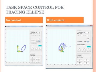
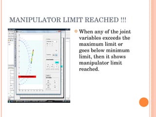
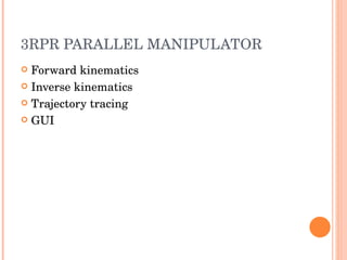
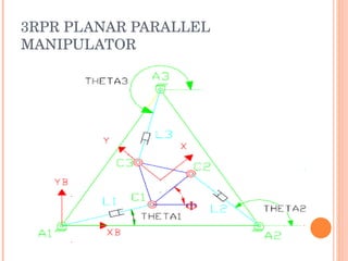
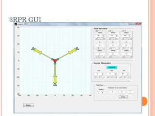
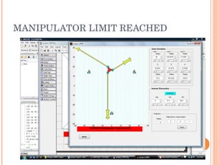
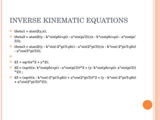
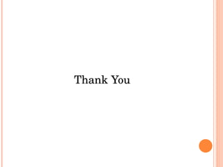
The document discusses the forward and inverse kinematics, trajectory tracking, and control of 3RPR planar parallel manipulators. It describes developing the homogeneous transformation matrices to draw link polygons in MATLAB. It also covers applying task space control for tracing circles and ellipses, and discusses reaching manipulator limits. Equations for the forward and inverse kinematics of the 3RPR parallel manipulator are provided. The approach for trajectory tracing using Jacobian matrices is outlined.

1. RPRP SERIAL CHAIN MANIPULATOR 3RPR PLANAR PARALLEL MANIPULATOR Sumit Tripathi Saket Kansara

2. RPRP serial chain manipulator Forward kinematics Inverse kinematics Trajectory tracking Circle Ellipse Task space control

3. RPRP GUI

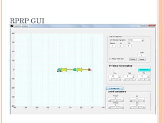
4. USE OF HOMOGENEOUS TRANSFORMATION TO DRAW LINK POLYGONS matlab_th1= theta1_g*pi/180; matlab_th2 = matlab_th1+theta2_g*pi/180; x1_t=x1_g*cos(matlab_th1); % So that prismatic joint 1 is always on top of revolute joint 1(circle) y1_t=y1_g+ r_g*sin(matlab_th1); Tm1 = [ cos(matlab_th1) -sin(matlab_th1) 0 x1_t % Transform to frame '1' sin(matlab_th1) cos(matlab_th1) 0 y1_t 0 0 1 0 0 0 0 1 ];

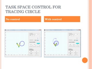
5. HOW DO WE APPLY CONTROL ?? xd=(xc+R*cos(w*t)); yd=(yc+R*sin(w*t)); ErrorX=[ (xd-x); (yd-y) ]; K=[g 0; 0 g]; error_correction = jacobian_i*K*ErrorX; qdot=jacobian_i*Xdot + error_correction ;

6. TASK SPACE CONTROL FOR TRACING CIRCLE No control With control

7. VARIATION OF RADIUS No control With control

8. TASK SPACE CONTROL FOR TRACING ELLIPSE No control With control

9. MANIPULATOR LIMIT REACHED !!! When any of the joint variables exceeds the maximum limit or goes below minimum limit, then it shows manipulator limit reached.

10. 3RPR PARALLEL MANIPULATOR

11. 3RPR PARALLEL MANIPULATOR Forward kinematics Inverse kinematics Trajectory tracing GUI

12. 3RPR PLANAR PARALLEL MANIPULATOR

13. 3RPR GUI

14. MANIPULATOR LIMIT REACHED

15. FORWARD KINEMATICS EQUATIONS m = (k*sin(theta2 - pi)*cos(theta1)*sin(theta3) )/(sin(theta2-theta1)) - (k*sin(theta2- pi)*sin(theta1)*cos(theta3))/(sin(theta2-theta1)) - k*cos(2*pi/3)*sin(theta3) - k*sin(2*pi/3)*cos(theta3); n = (-k*cos(theta2- pi)*cos(theta1)*sin(theta3))/(sin(theta2-theta1)) + (k*cos(theta2- pi)*sin(theta1)*cos(theta3))/(sin(theta2-theta1)) + k*sin(2*pi/3)*sin(theta3) - k*cos(2*pi/3)*cos(theta3); p = (-a*sin(theta2 - 2*pi/3)*cos(theta1)*sin(theta3))/(sin(theta2-theta1)) + (a*sin(theta2 - pi/3)*sin(theta1)*cos(theta3))/(sin(theta2-theta1)) + a*sin(theta3-2*pi/3); phi = 2*(atan2(-n + sqrt(n^2 -p^2 + m^2),(p-n))); x = (k*sin(theta2 - phi-pi) + a*sin(theta2-pi/3))*cos(theta1)/(sin(theta2-theta1)); y = (k*sin(theta2 - phi-pi) + a*sin(theta2-pi/3))*sin(theta1)/(sin(theta2-theta1)); d1 = sqrt(x^2 + y^2); d2 = sqrt((x- k*cos(phi+pi) - a*cos(pi/3))^2 + (y- k*sin(phi+pi)- a*sin(pi/3)) ^2) ; d3 = sqrt((x - k*cos(-2*pi/3-phi) + a*cos(2*pi/3))^2 + (y - k*sin(-2*pi/3-phi) + a*sin(2*pi/3))^2);

16. INVERSE KINEMATIC EQUATIONS theta1 = atan2(y,x); theta2 = atan2((y - k*sin(phi+pi) - a*sin(pi/3)),(x - k*cos(phi+pi) - a*cos(pi/3))); theta3 = atan2((y - k*sin(-2*pi/3-phi) - a*sin(2*pi/3)),(x - k*cos(-2*pi/3-phi) - a*cos(2*pi/3))); d1 = sqrt(x^2 + y^2); d2 = (sqrt((x- k*cos(phi+pi) - a*cos(pi/3))^2 + (y- k*sin(phi+pi)- a*sin(pi/3)) ^2)) ; d3 = (sqrt((x - k*cos(-2*pi/3-phi) + a*cos(2*pi/3))^2 + (y - k*sin(-2*pi/3-phi) + a*sin(2*pi/3))^2));

17. HOW TO DO TRAJECTORY TRACING ?? J1 = [ -d1*sin(theta1) cos(theta1) -k*sin(theta4); d1*cos(theta1) sin(theta1) k*cos(theta4); 1 0 1]; Similarly calculate J2 and J3; M = [ J1, -J2, zeros(3); J1, zeros(3), -J3]; theta_dependant_dot = -inv(M2)*M1*theta_independant_dot; M1 = matrix of rates of independent variables M2 = matrix of rates of dependent variables theta_dot = [ theta1_dot, d1_dot, theta4_dot, theta2_dot, d2_dot, theta5_dot, theta3_dot, d3_dot, theta6_dot ]'; Integrate theta_dot to get all the joint variables. Then use forward kinematics to plot.

18. Thank You