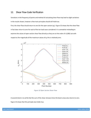
Downloaded 48 times
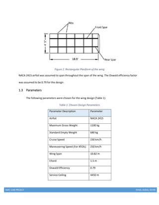
![MAE 154B PROJECT RYAN, AGRAJ, KEVIN
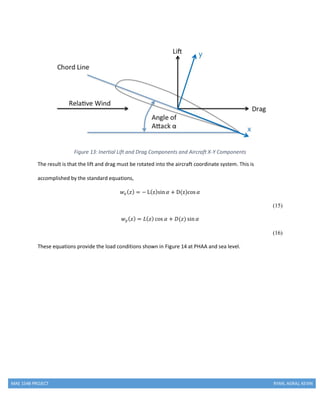
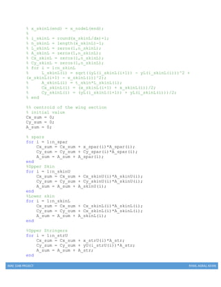
8. Centroid & Area Moments of Inertia
8.1 Cantilever Beam Model
The calculations for centroids and moments of inertia in relation to our wing design are all based
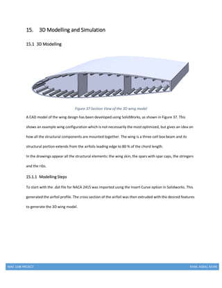
on the underlying assumption for the shape of the wing. We began our analysis by taking a simplified
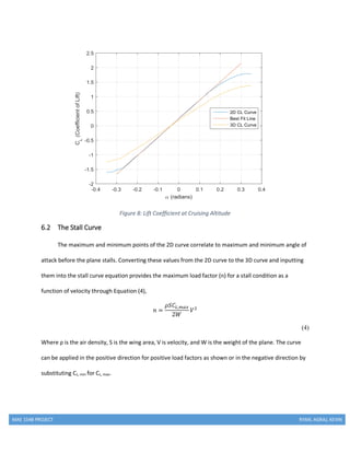
cross section of the wing (Figure 18). The design assumes a uniform cross section from root to tip. All
parts of the wing are also assumed to be composed of straight segments. The cross section is
approximated using three spars, eight brackets and four skin panels.
Table 3 Dimensions used in centroid & moment calculations
VARIABLE DIMENSIONS
Chord Length 1.5 m
Height 0.2235 m
SparThickness 0.0025 m
SkinThickness 0.001016 m
Spar Height 0.999797 m
Bracket Height 0.012 m
BracketThickness 0.0025 m
Theta 30 deg
Alpha 10 deg
Half Chord Length [m] 0.75
Half Height [m] 0.11175
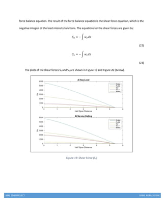
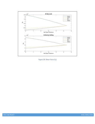
Half SparThickness [m] 0.00125
Half Spar Height [m] 0.4998985
Half BracketThickness [m] 0.00125
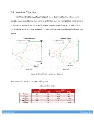
Theta [rad] 0.523598333](https://image.slidesharecdn.com/6e03d563-46c5-4e39-b180-83d24f29102e-170124015624/85/Report-Wing-Structure-Design-Spring-16-27-320.jpg)
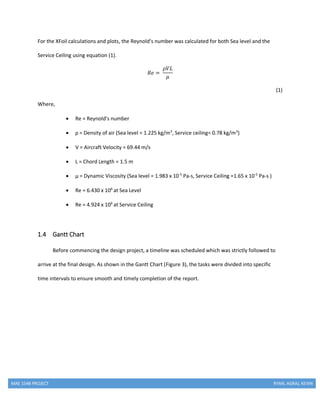
![MAE 154B PROJECT RYAN, AGRAJ, KEVIN
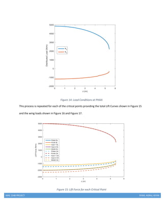
8.2 Centroid Calculations
Part of our project involved carrying out hand calculations to corroborate the results of our
MATLAB code. For the centroid calculation, many of the specifications were assumed to be the same as
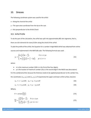
NACA 2412. Among them were: spar thickness (.0025 meters), skin thickness (.001016 meters) and the
area of the bracket (.0003 square meters). Other data was updated where applicable, such as chord
length (1.5 meters). We were given freedom over the location of the spars, and chose initial locations of
0 [m], 0.75 [m] and 1.5 [m]. Another assumption that we made was to assume that the brackets are
point masses located at the joint of the spar and the skin. In other words, the bracket height is
neglected. The bracket height is only used to calculate the area of the bracket in the cross section.
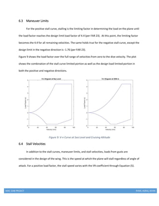
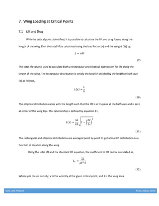
Figure 18: Simplified Wing Cross Section
In general, the centroid is calculated from an area-weighted average of the centroid of each of the
individual components. In our case this consists of 15 individual components. The MATLAB code
provided additional formulas to work with, some of which provided helpful assumptions in the
calculations. The x-coordinate of the centroid for the spars is set at their position coordinate on the
wing. The y-coordinate of the centroid for the spars is set to zero for root spar and middle spar, while
the spar out at the wing tip is calculated using trigonometry. This equation is given by:](https://image.slidesharecdn.com/6e03d563-46c5-4e39-b180-83d24f29102e-170124015624/85/Report-Wing-Structure-Design-Spring-16-28-320.jpg)
![MAE 154B PROJECT RYAN, AGRAJ, KEVIN
I 𝑥𝑦 = ∑ 𝐴𝑖 ∗ (
𝑛
𝑖=1
𝑥𝑖 − 𝑥̅) ∗ (𝑦𝑖 − 𝑦̅)
(21)
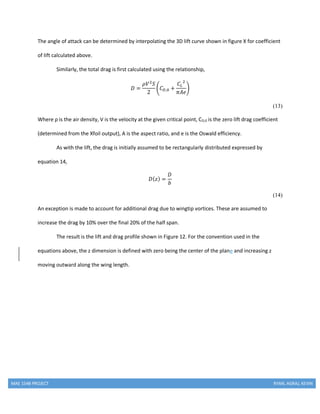
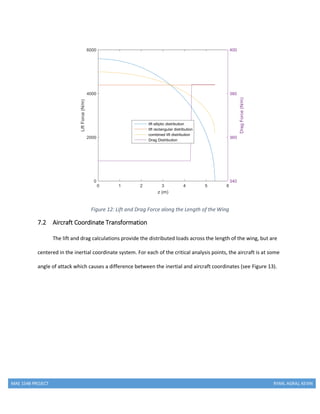
We used the formulas provided to calculate the area moment of inertia for the leading edge of the wing.
The values of Ixx, Iyy and Ixy for the entire wing are found by summing the values for the individual
components. The data used in the calculations for the three spars is shown in Table 5, the data for the
brackets in
Table 6 and the data for the wing’s skin in
. The net values for the leading edge of the wing are displayed in
Table 8.
Table 5: Spar Data
SPARS (3)
_
x
[m]
_
y
[m]
Area [m
2
]
Ixx
[m
4
]
Iyy
[m
4
]
Ixy
[m
4
]
1 0 0 0.00055875 0.00001103 0.00032871 -0.00005348
2 0.75 0 0.00055875 0.00001103 0.00000016 -0.00000119
3 1.5 -0.433 0.00055875 0.00005540 0.00030021 -0.00012623
Table 6: Bracket Data
BRACKETS (8)
_
x
[m]
_
y
[m]
Area [m
2
]
Ixx
[m
4
]
Iyy
[m
4
]
Ixy
[m
4
]
SKIN (4)
_
x
[m]
_
y
[m]
Area [m
2
]
Ixx
[m
4
]
Iyy
[m
4
]
Ixy
[m
4
]
1 top 0.375 0.1118 0.000762 4.26E-05 0.00015 -7.066E-05
1 bottom 0.375 -0.1118 0.000762 1.3E-07 0.00015 -3.896E-06
2 top 1.125 -0.1048 0.00087988 1.41E-05 0.000154 -1.75E-05
2 bottom 1.125 -0.3283 0.00087988 5.02E-05 0.000154 -8.79E-05](https://image.slidesharecdn.com/6e03d563-46c5-4e39-b180-83d24f29102e-170124015624/85/Report-Wing-Structure-Design-Spring-16-30-320.jpg)
![MAE 154B PROJECT RYAN, AGRAJ, KEVIN
1 top 0.0013 0.1118 0.00003 1.679E-06 1.76E-05 -5.4E-06
1 bottom 0.0013 -0.1118 0.00003 5.103E-09 1.76E-05 -3E-07
2 top 0.74875 0.1118 0.00003 1.679E-06 9.99E-09 -1.3E-07
2 bottom 0.74875 -0.1118 0.00003 5.103E-09 9.99E-09 -7.1E-09
3 top 0.75125 0.1118 0.00003 1.679E-06 7.44E-09 -1.1E-07
3 bottom 0.75125 -0.1118 0.00003 5.103E-09 7.44E-09 -6.2E-09
4 top 1.49875 -0.3213 0.00003 1.158E-06 1.61E-05 -4.3E-06
4 bottom 1.49875 -0.5448 0.00003 5.291E-06 1.61E-05 -9.2E-06
Table 7: Wing Skin Data
Table 8: Area Moment of Inertia Results
Net Area Moment of Inertia [m
4
]
Ixx 0.00019600
Iyy 0.00131007
Ixy -0.00038037
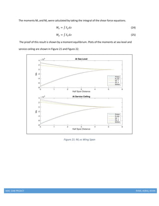
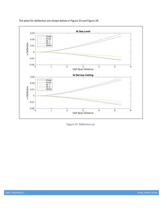
9. Shear Force, Bending, Deflection
This section of the report will go through the steps from load to deflection. Using the load intensity
equations calculated for wx and wy. The equation for shear force in the y-direction is found through a
SKIN (4)
_
x
[m]
_
y
[m]
Area [m
2
]
Ixx
[m
4
]
Iyy
[m
4
]
Ixy
[m
4
]
1 top 0.375 0.1118 0.000762 4.26E-05 0.00015 -7.066E-05
1 bottom 0.375 -0.1118 0.000762 1.3E-07 0.00015 -3.896E-06
2 top 1.125 -0.1048 0.00087988 1.41E-05 0.000154 -1.75E-05
2 bottom 1.125 -0.3283 0.00087988 5.02E-05 0.000154 -8.79E-05](https://image.slidesharecdn.com/6e03d563-46c5-4e39-b180-83d24f29102e-170124015624/85/Report-Wing-Structure-Design-Spring-16-31-320.jpg)
![MAE 154B PROJECT RYAN, AGRAJ, KEVIN
Figure 22: My vs Wing Span
The equations for u’’ and v’’ are given by equations 26 and 27:
𝑑2 𝑢
𝑑𝑧2 = −𝐾 ∗ [−𝑀𝑥 ∗ 𝐼𝑥𝑦 + 𝑀 𝑦 ∗ 𝐼𝑥𝑥] (26)
𝑑2 𝑣
𝑑𝑧2 = −𝐾 ∗ [𝑀𝑥 ∗ 𝐼 𝑦𝑦 − 𝑀 𝑦 ∗ 𝐼𝑥𝑦] (27)
𝐾 =
1
𝐸∗(𝐼 𝑥𝑥∗𝐼 𝑦𝑦−𝐼 𝑥𝑦
2 )
(28)
The deflections due to bending are found by integrating u’’ and v’’ twice. The constants of integration go
to zero because we integrate from the LHS. Ultimately, we compare the deflections at the tip by
executing numerical integration in MATLAB with equations 29 and 30:
𝑢( 𝑧) = ∑
𝑑𝑢
𝑑𝑧
∗ (𝑧𝑖+1 − 𝑧𝑖) (29)
𝑣( 𝑧) = ∑
𝑑𝑣
𝑑𝑧
∗ (𝑧𝑖+1 − 𝑧𝑖) (30)](https://image.slidesharecdn.com/6e03d563-46c5-4e39-b180-83d24f29102e-170124015624/85/Report-Wing-Structure-Design-Spring-16-35-320.jpg)
![MAE 154B PROJECT RYAN, AGRAJ, KEVIN
𝐼 𝑥′,𝑖 is the Area MOI of the ith
component about its own centroid about the x-axis (Negligible)
𝐼 𝑦′,𝑖 is the Area MOI of the ith
component about its own centroid about the y-axis (Negligible)
11. Shear Flow – Calculations
Using the calculated x-y coordinates to define the profile of the wing and the associated areas at each
point for spar caps and stringers, shear flow throughout the structure can be determined. Ideally, the
coordinate system would be centered at the centroid of the cross section, but this can be corrected for
through a simple coordinate transfer. Each point will be treated as a boom where the area of the boom
corresponds to the effective area of the skin, stringers, or spar caps adjacent to that point. This is
calculated such that axial stress is conserved between the actual cross section and the simplified boom
cross section. The final equation is shown in Equation (39).
𝐴 𝐵𝑜𝑜𝑚 = 𝐴 𝑠𝑝𝑎𝑟 𝑐𝑎𝑝 𝑜𝑟 𝑠𝑡𝑟𝑖𝑛𝑔𝑒𝑟 + ∑ [
𝑡𝑏
6
(2 +
𝜎 𝑧𝑧(𝑛+1)
𝜎 𝑧𝑧(𝑛)
)]𝑛
𝑖=1 (39)
Where the area of the spar cap or stringer are only for that specific point, n is the number of adjacent
panels, t is the thickness of that adjacent panel, b is the length of the adjacent panel, σzz(n+1) is the stress
at the point on the other end of the adjacent panel, and σzz is the stress at the current point. Typically n
is equal to 2, one for each of the adjacent skin panels. However at the locations where the spar meets
the skin, n is equivalent to 3 to include the contributions due to the spar. σzz in this equation is calculated
using the moment in the X and Y directions and implemented into Equation (40).
𝜎𝑧𝑧,𝑖 =
𝑀 𝑥(𝐼 𝑦𝑦(𝑦 𝑖−𝑦 𝑐)−𝐼 𝑥𝑦(𝑥 𝑖−𝑥 𝑐))
𝐼 𝑥𝑥 𝐼 𝑦𝑦−𝐼 𝑥𝑦
2 +
𝑀 𝑦(𝐼 𝑥𝑥(𝑥 𝑖−𝑥 𝑐)−𝐼 𝑥𝑦(𝑦 𝑖−𝑦 𝑐))
𝐼 𝑥𝑥 𝐼 𝑦𝑦−𝐼 𝑥𝑦
2 (40)
Where the moments of inertia are the previously calculated inertia terms for the wing cross section, x
and y are the coordinates of the point, and xc and yc are the x-y coordinates of the centroid if the points
are not already normalized.](https://image.slidesharecdn.com/6e03d563-46c5-4e39-b180-83d24f29102e-170124015624/85/Report-Wing-Structure-Design-Spring-16-42-320.jpg)
![MAE 154B PROJECT RYAN, AGRAJ, KEVIN
Figure 29 Shear Flow Idealization
Starting with point 1, the Δqb, or change in sheer flow from one side of the boom to the other is
calculated at each point around the profile using Equation (41).
Δ𝑞 𝑏,𝑖 =
𝑆 𝑦 𝐼 𝑥𝑦−𝑆 𝑥 𝐼 𝑥𝑥
𝐼 𝑥𝑥 𝐼 𝑦𝑦−𝐼 𝑥𝑦
2 𝐴 𝐵𝑜𝑜𝑚,𝑖( 𝑥𝑖 − 𝑥 𝑐) +
𝑆 𝑥 𝐼 𝑥𝑦−𝑆 𝑦 𝐼 𝑦𝑦
𝐼 𝑥𝑥 𝐼 𝑦𝑦−𝐼 𝑥𝑦
2 𝐴 𝐵𝑜𝑜𝑚,𝑖( 𝑦𝑖 − 𝑦𝑐) (41)
Where Sx and Sy are the shear forces, ABoom,I is the effective boom area at that point, xi and yi are the x-y
components of the point, and xc and yc are the centroid coordinates if not normalized. From this the
total qb at a given point is the sum of the Δqb’s for all previous points as shown in equation X. The values
of qb are shown in the Appendix.
𝑞 𝑏,𝑘 = ∑ Δ𝑞 𝑏,𝑖
𝑘
𝑖=1 (42)
To calculate the total q, the relationship between cell 1 and cell 2 must be accounted for. This is
considered by examining the total moment on the system in Equation (43) and the twist rate of each cell
using Equations (44) and (45).
𝑀0 + 𝑆 𝑦 𝜉0 − 𝑆 𝑥 𝜂0 = 2𝐴1 𝑞0,1 + 2𝐴2 𝑞0,2 + ∑ 2𝑞 𝑏,𝑖Δ𝐴𝑖
𝑛
𝑖=1 (43)
𝑑𝜃
𝑑𝑧
=
1
2𝐴1 𝐺
[𝑞0,1 (∑
((𝑥 𝑖+1−𝑥 𝑖)2+(𝑦 𝑖+1−𝑦 𝑖)2)
1
2
𝑡 𝑠𝑘𝑖𝑛
𝑛
𝑖=1 ) + (𝑞0,1 − 𝑞0,2)
(𝑦 𝑏𝑜𝑡−𝑦𝑡𝑜𝑝)
𝑡 𝑠𝑝𝑎𝑟
+
(𝑆 𝑦 𝐼 𝑥𝑦−𝑆 𝑥 𝐼 𝑥𝑥)
𝐼 𝑥𝑥 𝐼 𝑦𝑦−𝐼 𝑥𝑦
2 ∑ 𝐴 𝑏𝑜𝑜𝑚,𝑖 𝑥𝑖
((𝑥 𝑖+1−𝑥 𝑖)2+(𝑦 𝑖+1−𝑦 𝑖)2)
1
2
𝑡 𝑠𝑘𝑖𝑛
𝑛
𝑖=1 +
(𝑆 𝑥 𝐼 𝑥𝑦−𝑆 𝑦 𝐼 𝑦𝑦)
𝐼 𝑥𝑥 𝐼 𝑦𝑦−𝐼 𝑥𝑦
2 ∑ 𝐴 𝑏𝑜𝑜𝑚,𝑖 𝑦𝑖
((𝑥 𝑖+1−𝑥 𝑖)2+(𝑦 𝑖+1−𝑦 𝑖)2)
1
2
𝑡 𝑠𝑘𝑖𝑛
𝑛
𝑖=1 ]
(44)](https://image.slidesharecdn.com/6e03d563-46c5-4e39-b180-83d24f29102e-170124015624/85/Report-Wing-Structure-Design-Spring-16-44-320.jpg)
![MAE 154B PROJECT RYAN, AGRAJ, KEVIN
𝑑𝜃
𝑑𝑧
=
1
2𝐴2 𝐺
[𝑞0,2 (∑
((𝑥 𝑖+1−𝑥 𝑖)2+(𝑦 𝑖+1−𝑦 𝑖)2)
1
2
𝑡 𝑠𝑘𝑖𝑛
𝑛
𝑖=1 ) + (𝑞0,2 − 𝑞0,1)
(𝑦𝑡𝑜𝑝−𝑦 𝑏𝑜𝑡)
𝑡 𝑠𝑝𝑎𝑟
+ 𝑞0,2
(𝑦𝑡𝑜𝑝−𝑦 𝑏𝑜𝑡)
𝑡 𝑠𝑝𝑎𝑟
+
(𝑆 𝑦 𝐼 𝑥𝑦−𝑆 𝑥 𝐼 𝑥𝑥)
𝐼 𝑥𝑥 𝐼 𝑦𝑦−𝐼 𝑥𝑦
2 ∑ 𝐴 𝑏𝑜𝑜𝑚,𝑖 𝑥𝑖
((𝑥 𝑖+1−𝑥 𝑖)2+(𝑦 𝑖+1−𝑦 𝑖)2)
1
2
𝑡 𝑠𝑘𝑖𝑛
𝑛
𝑖=1 +
(𝑆 𝑥 𝐼 𝑥𝑦−𝑆 𝑦 𝐼 𝑦𝑦)
𝐼 𝑥𝑥 𝐼 𝑦𝑦−𝐼 𝑥𝑦
2 ∑ 𝐴 𝑏𝑜𝑜𝑚,𝑖 𝑦𝑖
((𝑥 𝑖+1−𝑥 𝑖)2+(𝑦 𝑖+1−𝑦 𝑖)2)
1
2
𝑡 𝑠𝑘𝑖𝑛
𝑛
𝑖=1 ]
(45)
It can be assumed that the wing cross section behaves as a rigid body and thus the twist rates are
equivalent. This leaves three equations with three unknowns; dθ/dz, q0,1, and q0,2. Solving the system of
equations gives the q0,1 and q0,2 to complete Equation (46).
𝑞𝑡𝑜𝑡𝑎𝑙,𝑖 = 𝑞 𝑏,𝑖 + 𝑞0,1 𝑜𝑟 2 (46)
Where the q0 is the appropriate term for the cell containing the point in question. This resulting shear
flow (qtotal) is in terms of the shear force per unit length. To get this into shear stress, the shear flow
must be divided by the thickness, resulting in units of shear force per unit area (Equation (47)).
𝜎𝑧𝑠,𝑖 =
𝑞 𝑡𝑜𝑡𝑎𝑙,𝑖
𝑡 𝑠𝑘𝑖𝑛
(47)
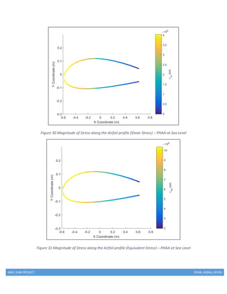
Combining the shear stress and the axial stress from Equation (47) at each point, the equivalent
principle stress can be calculated. Equation (48) defines this relationship.
𝜎𝑒𝑞,𝑖 = √2𝜎𝑧𝑧,𝑖
2 + 6𝜎𝑧𝑠,𝑖
2 (48)
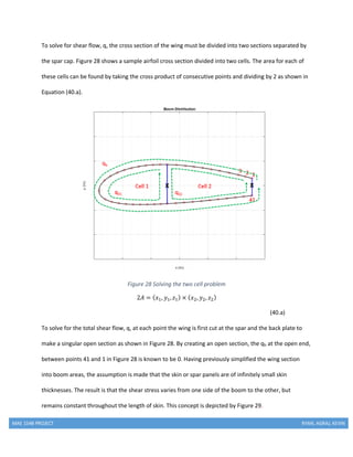
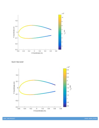
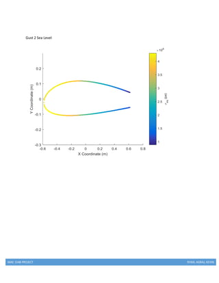
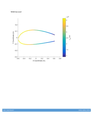
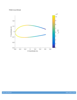
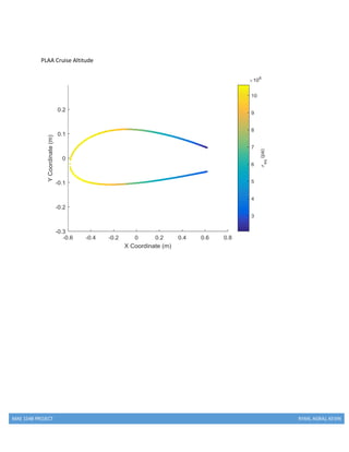
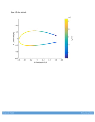
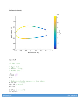
11.1 Shear Flow – Results
The results of these calculations for the first of the 10 critical points being analyzed (PHAA at Sea Level)
can be seen in Figure 30, shear stress, and Figure 31, equivalent stress. As the legend on the right
indicates, the colors correspond to the magnitude of the stress at that location.](https://image.slidesharecdn.com/6e03d563-46c5-4e39-b180-83d24f29102e-170124015624/85/Report-Wing-Structure-Design-Spring-16-45-320.jpg)
![MAE 154B PROJECT RYAN, AGRAJ, KEVIN
Figure 33 Product of Shear Flow and Boom Area
13.Buckling, Fatigue & Von Mises Stress
13.1 Von Mises Stresses
An important test in the design of our wing was to check the yield stress against the Von Mises
yield criterion. The tensile yield strength of AL 2024 T3 is 345 MPa and the ultimate tensile
strength is 483 MPa. The Von Mises equation is given in terms of principal stresses by equation
49 below.
𝜎𝑒𝑞 = √
[( 𝜎11 − 𝜎22)2 + ( 𝜎22 − 𝜎33)2 + ( 𝜎33 − 𝜎11)2 + 6( 𝜎12
2
+ 𝜎23
2
+ 𝜎31
2 )]
2
(49)](https://image.slidesharecdn.com/6e03d563-46c5-4e39-b180-83d24f29102e-170124015624/85/Report-Wing-Structure-Design-Spring-16-48-320.jpg)
![MAE 154B PROJECT RYAN, AGRAJ, KEVIN
In our analysis, equation 49 reduces to equation 50 because we only have one longitudinal
component and one shear component.
𝜎𝑒𝑞 = √
[2( 𝜎𝑧𝑧)2 + 6( 𝜎𝑧𝑠)2]
2
(50)
Table 9: Von Mises Stress Calculation
The calculation verifies that our wing design meets the Von Mises Yield Criterion with a factor of
safety of 1.4 for yield and 2.0 for fracture.
13.2 Column Buckling
We considered column buckling in our wing design to avoid stringer buckling, which is achieved
by adjusting the spacing of the ribs. The theory for the buckling analysis was worked out by Euler in
the eighteenth century. Euler’s equations for a load P applied to the ends of a beam can be seen in
the equations and Figure 34 below:
Figure 34: Column Buckling](https://image.slidesharecdn.com/6e03d563-46c5-4e39-b180-83d24f29102e-170124015624/85/Report-Wing-Structure-Design-Spring-16-49-320.jpg)
![MAE 154B PROJECT RYAN, AGRAJ, KEVIN
We use two equations to solve for the rib spacing:
𝑃𝐶𝑅 =
(𝜋2
𝐸𝐼)
𝑙 𝑒
2
(51)
The variables, their values, and the units for each term are outlined in tables 10 & 11 below.
𝑃𝐶𝑅 = 1.5𝜎𝑧𝑧 𝐴 𝑠𝑡𝑟𝑖𝑛𝑔𝑒𝑟
(52)
There is an n-squared factor in equation 51 that disappears when we set n equal to one (setting n equal
to one gives the smallest value for P where the column remains in equilibrium [Megson 271]). Next, by
setting equations (51) & (52) equal to each other and solving for effective length, we obtain the results
in Table 10.
Table 10: Rib Spacing
Table 11: Stringer Area
We use the following equation (53) from Megson [Table 8.1, pg. 272] to solve for the rib spacing given
the effective length:
𝑙 𝑒
𝑙
= 2 (53)
Setting Equation 53 equal to 2 gives us the most conservative value for rib spacing, as a larger effective
length decreases the value for P critical that yields failure in the column. Given a half-span of 5.41
meters, this would suggest 10 ribs evenly spaced along the wing.](https://image.slidesharecdn.com/6e03d563-46c5-4e39-b180-83d24f29102e-170124015624/85/Report-Wing-Structure-Design-Spring-16-50-320.jpg)
![MAE 154B PROJECT RYAN, AGRAJ, KEVIN
13.3 Skin (Thin Plate) Buckling
We consider thin plate buckling theory to determine the design for the skin plates that are
strengthened by the ribs and stringers. This analysis will compare the critical buckling load of the
individual plates with the total compressive plate buckling stress. The critical buckling load is given by
equation 54:
𝑁𝑋,𝐶𝑅 =
𝑘𝜋2
𝐸𝑡3
12𝑏2(1 − 𝑣2)
(54)
We set the buckling coefficient k equal to 8.5, set the Elastic Modulus for AL 2024 T3 to 73.1
[GPa], set Poisson’s ratio, v, equal to 0.33, while t and b are the skin thickness and plate length,
respectively. Next, we summed the critical buckling load for each section and divided by the skin
thickness to find the total compressive plate buckling stress.
𝜎 𝐶𝑅 =
𝑛 ∗ 𝑁𝑋,𝐶𝑅
𝑡
(55)
Here n is the number of plates, and t is the skin thickness. The calculations are shown in Table 12 below.
Table 12
13.4 Shear Buckling of Skin
In addition to column buckling and skin (thin plate) buckling, plate buckling from shear loading
of the wing’s skin was considered. The coefficient, k, used for plate buckling from shear loading is
given by Figure 35. Using the appropriate value for k, the buckling stress is calculated using
equation 54. With the calculated values for shear stress in the skin below the critical buckling
stress, the geometry of the wing design passed this test.](https://image.slidesharecdn.com/6e03d563-46c5-4e39-b180-83d24f29102e-170124015624/85/Report-Wing-Structure-Design-Spring-16-51-320.jpg)
![MAE 154B PROJECT RYAN, AGRAJ, KEVIN
Figure 35: Shear Buckling Coefficients for Flat Plates (Megson 315)
13.5 Fracture & Fatigue
Fatigue is defined as the progressive deterioration of the strength of a material or structural
component during service such that failure can occur at much lower stress levels than the
ultimate stress level [Megson 455]. Fracture can also occur at stresses below the yield stress if an
initial crack is present. A small crack, if undetected, can manifest into catastrophic failure. Figure
36 below from Megson (pg. 423) illustrates the reduction in failure stress as the number of
repetitions of this stress increases.
Figure 36 Failure Stress vs Number of Loading repetitions
Here we analyze the number of flight cycles our wing can endure before a crack grows by 1.8
centimeters, given an initial crack size of 0.2 centimeters.](https://image.slidesharecdn.com/6e03d563-46c5-4e39-b180-83d24f29102e-170124015624/85/Report-Wing-Structure-Design-Spring-16-52-320.jpg)
![MAE 154B PROJECT RYAN, AGRAJ, KEVIN
The equation for the number of loading/flight cycles (N) until failure is given by Equation 56:
𝑁 =
𝑎 𝐶𝑅
1−
𝑚
2
− 𝑎𝑖
1−
𝑚
2
𝐶(1 −
𝑚
2 )𝜋2 𝜎∞
2
(56)
To solve for aCR, we plug in a value for KIC (26 [MPa*m^.5]) into Equation (57)
𝑎 𝐶𝑅 =
1
𝜋
(
𝐾𝐼𝐶
𝜎∞
)2
(57)
The results are given in Error! Reference source not found.. The critical crack length is calculated as
approximately 5.4mm.
Table 13: Flight Cycles to Failure
14. Aeroelasticity
14.1 Divergence
Wing divergence is the process of an applied load increasing due to aerodynamic loads (i.e. a
positive torsional pitch moment) that eventually build and cause the wing to reach a divergence
point. The deflection due to the increasing load causes the angle of attack to increase, and the
increasing wing deflection and twist this creates can lead to failure. The torsional divergence
speed is calculated from equation 58, where U is the torsional divergence speed:
𝑀 = 𝐶𝑈2
(𝜃 + 𝛼0)
(58)](https://image.slidesharecdn.com/6e03d563-46c5-4e39-b180-83d24f29102e-170124015624/85/Report-Wing-Structure-Design-Spring-16-53-320.jpg)

![MAE 154B PROJECT RYAN, AGRAJ, KEVIN
W=1100*9.8; % Newtons
rho0=1.225; % Kg/m^3
rhoC=.7809; % Kg/m^3
VC=230*1000/3600; % m/s
VD=VC*1.5; % m/s
V=[0:0.5:VD]; % m/s
mu=1.983e-5; % pa*sec
g=32.17; % ft/s^2
A_cap=.0003; % m^2
A_str=.0001; % m^2
t_spar=.0025; % m
t_skin= .001; % m
x_spar=c/3; % m
x_strU=[0:5:95]*1.2/100; % m
x_strL=x_strU; % m
G=27579029160; % pa for 2024 all tempers
% Calculate a Reynolds Number
Re0=rho0*VC*c/mu;
ReC=rhoC*VC*c/mu;
[alpha1,CL1,CD1,CDp1,CM1,Top_Xtr1,Bot_Xtr1]=textread('naca24150.
pol','%f %f %f %f %f %f %f','headerlines', 12);
[alpha2,CL2,CD2,CDp2,CM2,Top_Xtr2,Bot_Xtr2]=textread('naca2415C.
pol','%f %f %f %f %f %f %f','headerlines', 12);
alpha={alpha1,alpha2};
CL={CL1,CL2};
CD={CD1,CD2};
CDp={CDp1,CDp2};
CM={CM1,CM2};
Top_Xtr={Top_Xtr1,Top_Xtr2};
Bot_Xtr={Bot_Xtr1,Bot_Xtr2};
alphar{1}=deg2rad(alpha{1});
alphar{2}=deg2rad(alpha{2});
ind=find(CL{1}>0,1);
CD0(1)=CD{1}(ind);
clear ind
ind=find(CL{2}>0,1);
CD0(2)=CD{2}(ind);
clear ind](https://image.slidesharecdn.com/6e03d563-46c5-4e39-b180-83d24f29102e-170124015624/85/Report-Wing-Structure-Design-Spring-16-71-320.jpg)
![MAE 154B PROJECT RYAN, AGRAJ, KEVIN
[CLmax(1),mind(1)]=max(CL{1});
[CLmin(1),mind(2)]=min(CL{1});
[CLmax(2),mind(3)]=max(CL{2});
[CLmin(2),mind(4)]=min(CL{2});
Vspos(1)=sqrt(2*W/(CLmax(1)*rho0*S));
Vsneg(1)=sqrt(2*W/(abs((1))*rho0*S));
Vspos(2)=sqrt(2*W/(CLmax(2)*rhoC*S));
Vsneg(2)=sqrt(2*W/(abs(CLmin(2))*rhoC*S));
ind1(1)=find(alpha{1}==-7);
ind2(1)=find(alpha{1}==10);
ind1(2)=find(alpha{2}==-7);
ind2(2)=find(alpha{2}==10);
linefit(1,:)=polyfit(alphar{1}(ind1(1):ind2(1)),CL{1}(ind1(1):in
d2(1)),1);
linefit(2,:)=polyfit(alphar{2}(ind1(2):ind2(2)),CL{2}(ind1(2):in
d2(2)),1);
x=linspace(-.3,.3)';
y(:,1)=linefit(1,1).*x+linefit(1,2);
xinter(:,1)=-linefit(1,2)/linefit(1,1);
y(:,2)=linefit(2,1).*x+linefit(2,2);
xinter(:,2)=-linefit(2,2)/linefit(2,1);
CL3Dslope(1,1)=linefit(1,1)/(1+linefit(1,1)/(pi*A*e));
CL3Dline(1,1)=CL3Dslope(1,1);
CL3Dline(1,2)=-CL3Dslope(1,1)*xinter(:,1);
CL3Dslope(2,1)=linefit(2,1)/(1+linefit(2,1)/(pi*A*e));
CL3Dline(2,1)=CL3Dslope(2,1);
CL3Dline(2,2)=-CL3Dslope(2,1)*xinter(:,2);
CLmax(1)=CLmax(1)*CL3Dline(1,1)/linefit(1,1);
CLmin(1)=CLmin(1)*CL3Dline(1,1)/linefit(1,1);
CLmax(2)=CLmax(2)*CL3Dline(2,1)/linefit(2,1);
CLmin(2)=CLmin(2)*CL3Dline(2,1)/linefit(2,1);
% CLmax(1)=CL3Dline(1,1)*alphar{1}(mind(1))+CL3Dline(1,2);
% CLmin(1)=CL3Dline(1,1)*alphar{1}(mind(2))+CL3Dline(1,2);
% CLmax(2)=CL3Dline(2,1)*alphar{2}(mind(3))+CL3Dline(2,2);
% CLmin(2)=CL3Dline(2,1)*alphar{2}(mind(4))+CL3Dline(2,2);
% y3D(:,1)=CL3Dline(1,1).*x+CL3Dline(1,2);
% y3D(:,2)=CL3Dline(2,1).*x+CL3Dline(2,2);
y3Dline1{1}=(CL3Dline(1,1)/linefit(1,1)).*CL{1};](https://image.slidesharecdn.com/6e03d563-46c5-4e39-b180-83d24f29102e-170124015624/85/Report-Wing-Structure-Design-Spring-16-72-320.jpg)
![MAE 154B PROJECT RYAN, AGRAJ, KEVIN
for j=1:2
maxpos(j)=max(nposi{j});
maxneg(j)=max(nnegi{j});
npos(maxpos(j)+1:end,j)=4.4;
nneg(maxneg(j)+1:nnegi{3},j)=-1.76;
for n=nnegi{3}:length(V)
nneg(n,j)=manslope*V(n)+manint;
end
end
npos(end+1,:)=zeros(1,2);
nneg(end+1,:)=zeros(1,2);
V(end+1)=V(end);
%% Calculate the Gust Load Factor
UeC=50; % ft/s
UeD=25; % ft/s
VCk=VC*1.944; % knots
VDk=VD*1.944; % knots
cft=c*3.28084; % ft
Wlbf=W*0.224809; % lbf
Sft2=S*10.7639; % ft^2
rho0s=rho0*0.00194032; % slug/ft^3
rhoCs=rhoC*0.00194032; % slug/ft^3
u0=2*Wlbf/Sft2/(rho0s*cft*CL3Dslope(1)*g);
uC=2*Wlbf/Sft2/(rhoCs*cft*CL3Dslope(2)*g);
Kg0=.88*u0/(5.3+u0);
KgC=.88*uC/(5.3+uC);
nC(1)=1+Kg0*CL3Dslope(1)*UeC*VCk/(498*(Wlbf/Sft2));
nC(2)=1+KgC*CL3Dslope(2)*UeC*VCk/(498*(Wlbf/Sft2));
nD(1)=1+Kg0*CL3Dslope(1)*UeD*VDk/(498*(Wlbf/Sft2));
nD(2)=1+KgC*CL3Dslope(2)*UeD*VDk/(498*(Wlbf/Sft2));
ngustposS(:,1)=[1,nC(1),nD(1),1];
ngustnegS(:,1)=[1,-(nC(1)-2),-(nD(1)-2),1];
ngustposS(:,2)=[1,nC(2),nD(2),1];
ngustnegS(:,2)=[1,-(nC(2)-2),-(nD(2)-2),1];
vgust=[0,VC,VD,0];
ngustpos(:,1)=interp1(vgust(1:3),ngustposS(1:3,1),V);
ngustneg(:,1)=interp1(vgust(1:3),ngustnegS(1:3,1),V);](https://image.slidesharecdn.com/6e03d563-46c5-4e39-b180-83d24f29102e-170124015624/85/Report-Wing-Structure-Design-Spring-16-74-320.jpg)
![MAE 154B PROJECT RYAN, AGRAJ, KEVIN
ngustpos(:,2)=interp1(vgust(1:3),ngustposS(1:3,2),V);
ngustneg(:,2)=interp1(vgust(1:3),ngustnegS(1:3,2),V);
count=0;
countn=0;
for j=1:2
for n=1:length(V)
if V(n)<Vspos(j)
else
count=count+1;
Vcomp{j}(count)=V(n);
end
if V(n)>Vspos(j)&& n<=maxpos(j)
nComp{j}(count)=npos(n,j);
elseif n>maxpos(j)
nComp{j}(count)=max(npos(n,j),ngustpos(n,j));
end
if V(n)<Vsneg(j)
else
countn=countn+1;
Vcomn{j}(countn)=V(n);
end
if V(n)>Vsneg(j)&&n<=maxneg(j)
nComn{j}(countn)=nneg(n,j);
elseif n>maxneg(j)
nComn{j}(countn)=min(nneg(n,j),ngustneg(n,j));
end
end
count=0;
countn=0;
end
nComp{1}=[0,nComp{1},0];
Vcomp{1}=[Vspos(1),Vcomp{1},VD];
nComp{2}=[0,nComp{2},0];
Vcomp{2}=[Vspos(2),Vcomp{2},VD];
nComn{1}=[0,0,nComn{1},0];
Vcomn{1}=[Vspos(1),Vsneg(1),Vcomn{1},VD];
nComn{2}=[0,0,nComn{2},0];
Vcomn{2}=[Vspos(2),Vsneg(2),Vcomn{2},VD];
figure('Position',[50,50,1200,500])
subplot(1,2,1)
plot(V,npos(:,1),'b')
hold on
plot(vgust,ngustposS(:,1),'r')](https://image.slidesharecdn.com/6e03d563-46c5-4e39-b180-83d24f29102e-170124015624/85/Report-Wing-Structure-Design-Spring-16-75-320.jpg)
![MAE 154B PROJECT RYAN, AGRAJ, KEVIN
plot(Vcomp{1},nComp{1},'g--','linewidth',2)
plot(V,nneg(:,1),'b')
plot(vgust,ngustnegS(:,1),'r')
plot(Vcomn{1},nComn{1},'g--','linewidth',2)
legend('Maneuver Limit','Gust Loading','Combined
Loading','Location','northwest')
title('V-n Diagram at Sea Level')
xlabel('Velocity (m/s)')
ylabel('Load Factor (n)')
subplot(1,2,2)
plot(V,npos(:,2),'b')
hold on
plot(vgust,ngustposS(:,2),'r')
plot(Vcomp{2},nComp{2},'g--','linewidth',2)
plot(V,nneg(:,2),'b')
plot(vgust,ngustnegS(:,2),'r')
plot(Vcomn{2},nComn{2},'g--','linewidth',2)
legend('Maneuver Limit','Gust Loading','Combined
Loading','Location','northwest')
title('V-n Diagram at 4450 m')
xlabel('Velocity (m/s)')
ylabel('Load Factor (n)')
%% Calculating Wx and Wy
LCs=[59.5 4.4
95.5 4.4
95.5 -1.1
64 -1.78
39.5 -1.76
75.5 4.4
95.5 4.4
95.5 -1.298
64 -2.051
50.5 -1.76];
nz=100;
for n=1:length(LCs)
if n>length(LCs)/2
rho=rhoC;
CD0T=CD0(2);
m=2;
else
rho=rho0;
CD0T=CD0(1);](https://image.slidesharecdn.com/6e03d563-46c5-4e39-b180-83d24f29102e-170124015624/85/Report-Wing-Structure-Design-Spring-16-76-320.jpg)
![MAE 154B PROJECT RYAN, AGRAJ, KEVIN
m=1;
end
L(n) = LCs(n,2)*W; % N
lift
CLCP(n) = 2*L(n)/rho/LCs(n,1)^2/S; %
lift coefficient
% Alpha(n)=(CLCP(n)-CL3Dline(2))/CL3Dline(1);
Alpha(n)=interp1(y3Dline1{m},alphar{m},CLCP(n));
D(n) = 0.5*rho*LCs(n,1)^2*S*(CD0(m) + CLCP(n)^2/pi/A/e); %
N drag
z = 0:b/2/nz:b/2; % root to tip (half
span)
% lift distribution
l_rect(:,n) = L(n)/b.*ones(1,nz+1);
l_ellip (:,n)= (4*L(n)/pi/b).*sqrt(1-(2.*z./b).^2);
l (:,n)= (l_rect(:,n) + l_ellip(:,n))./2; %
N/m
d (:,n)=D(n)/b.*ones(1,nz+1);
for m=1:length(d)
if m>.8*length(d)
d(m,n)=d(m,n)*1.1;
end
end
figure('Position',[50,50,1200,500])
subplot(1,2,1)
p=plotyy([z',z',z'],[l_ellip(:,n),l_rect(:,n),l(:,n)],z,d(:,n));
ylabel(p(1),'Lift Force (N/m)')
xlabel('z (m)')
ylabel(p(2),'Drag Force (N/m)')
legend('lift elliptic distribution','lift rectangular
distribution','combined lift distribution','Drag
Distribution','location','best')
% rotate into x-y coordinate
wy(:,n) = cos(Alpha(n)).*l(:,n) + sin(Alpha(n)).*d(:,n);
wx(:,n) = -sin(Alpha(n)).*l(:,n) + cos(Alpha(n)).*d(:,n);
% Note: wx and wy are defined from root to tip
subplot(1,2,2)
plot(z,wy,z,wx,'linewidth',2)](https://image.slidesharecdn.com/6e03d563-46c5-4e39-b180-83d24f29102e-170124015624/85/Report-Wing-Structure-Design-Spring-16-77-320.jpg)
![MAE 154B PROJECT RYAN, AGRAJ, KEVIN
xlabel('z (m)')
ylabel('Distributed Load (N/m)')
legend('w_y','w_x','location','best')
end
figure('Position',[50,50,800,500])
plot(z,l(:,1),'-',z,l(:,2),'-',z,l(:,3),'-',z,l(:,4),'-
',z,l(:,5),'-',...
z,l(:,6),'--',z,l(:,7),'--',z,l(:,8),'--',z,l(:,9),'--
',z,l(:,10),'--','linewidth',2)
ylabel('Lift Force (N/m)')
xlabel('z (m)')
legend('PHAA SL','PLAA SL','Gust 1 SL','Gust 2 SL','NHAA
SL','PHAA CA','PLAA CA','Gust 1 CA','Gust 2 CA','NHAA
CA','location','west')
Rho(1:5)=rho0;
Rho(6:10)=rhoC;
Cd(1:5)=CD(1);
Cd(6:10)=CD(2);
for n=1:length(LCs)
[z1t,Mx0t,My0t,Sx0t,Sy0t,sig_z0t,u0t,v0t] =
DeflectionLoadscode(wx(:,n),wy(:,n),LCs(n,2),Rho(n),LCs(n,1),Alp
ha(n),Cd(n),nz);
z1(:,n)=z1t;
Mx0(:,n)=Mx0t;
My0(:,n)=My0t;
Sx0(:,n)=Sx0t;
Sy0(:,n)=Sy0t;
sig_z0(:,n)=sig_z0t;
u0a(:,n)=u0t;
v0a(:,n)=v0t;
clear z1t Mx0t My0t Sx0t Sy0t sig_z0t u0t v0t
end
%% X Moments
figure
subplot(2,1,1)
plot(z,Mx0(:,1),z,Mx0(:,2),z,Mx0(:,3),z,Mx0(:,4),z,Mx0(:,5))
legend('PHAA','PLAA','GL 1','GL 2','NHAA','location','best')
ylabel('Mx')
xlabel('Half Span Distance')
title('At Sea Level')
subplot(2,1,2)
plot(z,Mx0(:,6),z,Mx0(:,7),z,Mx0(:,8),z,Mx0(:,9),z,Mx0(:,10))
legend('PHAA','PLAA','GL 1','GL 2','NHAA','location','best')](https://image.slidesharecdn.com/6e03d563-46c5-4e39-b180-83d24f29102e-170124015624/85/Report-Wing-Structure-Design-Spring-16-78-320.jpg)
![MAE 154B PROJECT RYAN, AGRAJ, KEVIN
subplot(2,1,2)
plot(z,v0a(:,6),z,v0a(:,7),z,v0a(:,8),z,v0a(:,9),z,v0a(:,10))
legend('PHAA','PLAA','GL 1','GL
2','NHAA','location','northeast')
ylabel('v-Deflection')
xlabel('Half Span Distance (m)')
title('At Service Ceiling')
%% Recalculating the Airfoil Section
[cq,Ixx,Iyy,Ixy,x,yU,yL,Bigmat,i_strU,dx,i_spar,i_strL] =
airfoil_section(c,A_cap,A_str,t_spar,t_skin,x_spar,x_strU,x_strL
);
Ivals=[Ixx,Iyy,Ixy];
for n=1:length(LCs)
SMvals=[Mx0(1,n),My0(1,n),Sx0(1,n),Sy0(1,n)]; % at the root
[sigeq(:,n),sigzs(:,n),sigzz(:,n),qtot(:,n),xyc,xycent,qb(:,n),s
igcheck(:,n)]=shearflow(Bigmat,cq,SMvals,Ivals,t_skin,t_spar,G);
figure
scatter(xycent(:,1),xycent(:,2),10,sigzs(:,n),'filled')
c=colorbar;
c.Label.String='sigma_z_s (pa)';
ylim ([-.3 .3])
xlabel('X Coordinate (m)')
ylabel('Y Coordinate (m)')
figure
scatter(xycent(:,1),xycent(:,2),10,sigeq(:,n),'filled')
c=colorbar;
c.Label.String='sigma_e_q (pa)';
ylim ([-.3 .3])
xlabel('X Coordinate (m)')
ylabel('Y Coordinate (m)')
end
figure
scatter(xycent(:,1),xycent(:,2),10,sigeq(:,1),'filled')
c=colorbar;
c.Label.String='sigma_e_q';
ylim ([-.3 .3])](https://image.slidesharecdn.com/6e03d563-46c5-4e39-b180-83d24f29102e-170124015624/85/Report-Wing-Structure-Design-Spring-16-81-320.jpg)
![MAE 154B PROJECT RYAN, AGRAJ, KEVIN
xlabel('X Coordinate (m)')
ylabel('Y Coordinate (m)')
figure
plot(x,yU,'k','Linewidth',2);
ylim([-0.3 0.3])
hold on
plot(i_strU*dx,yU(i_strU),'or','markersize',5);
plot([x_spar(1),x_spar(1)],[yU(i_spar(1)),yL(i_spar(1))],'b','Li
newidth',3);
scatter(xyc(1,1),xyc(1,2),'m*')
plot(x,yL,'k','Linewidth',2);
plot(i_strL*dx,yL(i_strL),'or','markersize',5);
plot([x(end),x(end)],[yU(end),yL(end)],'b','Linewidth',3);
ylabel('y (m)')
xlabel('x (m)')
grid on
legend('Airfoil','Stringers','Spars','Centriod')
figure
plot(qb)
ylabel('q_b (N/m)')
xlabel('Point Number')
legend('PHAA SL','PLAA SL','Gust 1 SL','Gust 2 SL','NHAA
SL','PHAA CA','PLAA CA','Gust 1 CA','Gust 2 CA','NHAA
CA','location','best')
figure
plot(sigcheck)
ylabel('Sigma_z_s*Boom Area (lbf)')
xlabel('Point Number')
legend('PHAA SL','PLAA SL','Gust 1 SL','Gust 2 SL','NHAA
SL','PHAA CA','PLAA CA','Gust 1 CA','Gust 2 CA','NHAA
CA','location','best')
function[sigeq,sigzs,sigzz,qtot,xyc,xycent,q,sigcheck]=shearflow
(Bigmat,xs,SMvals,Ivals,tskin,tspar,G)
xy=Bigmat(:,1:2);
if xy(1,2)~=xy(end,2)
xy(end+1,:)=xy(1,:);
end
b=ones(length(xy),1);](https://image.slidesharecdn.com/6e03d563-46c5-4e39-b180-83d24f29102e-170124015624/85/Report-Wing-Structure-Design-Spring-16-82-320.jpg)
![MAE 154B PROJECT RYAN, AGRAJ, KEVIN
xy=[xy,b*0];
% calculate area of wing cross section
for n=1:length(xy)-1
dA2(n)=norm(cross(xy(n,:),xy(n+1,:)));
A2(n)=sum(dA2);
ldist(n,1)=sqrt((xy(n,1)-xy(n+1,1))^2+(xy(n,2)-
xy(n+1,2))^2);
askin(n,1)=Bigmat(n,6);
xyA(n,:)=[xy(n,1)*askin(n),xy(n,2)*askin(n)];
atot(n,1)=sum(Bigmat(n,3:6));
end
xyc(1,:)=[sum(xyA(:,1))/sum(askin),sum(xyA(:,2))/sum(askin)];
%normalize x and y vectors to centriod
xycent=xy-[b*xyc(1),b*xyc(2),b*0];
% calculate area of wing cross section
for n=1:length(xy)-1
dA2(n)=norm(cross(xycent(n,:),xycent(n+1,:)));
A2(n)=sum(dA2);
ldist(n,1)=sqrt((xycent(n,1)-xycent(n+1,1))^2+(xycent(n,2)-
xycent(n+1,2))^2);
askin(n,1)=Bigmat(n,6);
xyA(n,:)=[xycent(n,1)*askin(n),xycent(n,2)*askin(n)];
atot(n,1)=sum([Bigmat(n,3),Bigmat(n,5:6)]);
end
xyc(2,:)=[sum(xyA(:,1))/sum(askin),sum(xyA(:,2))/sum(askin)];
for n=1:length(xycent)-1
Ivec(n,:)=[askin(n)*(xycent(n,2)-
xyc(2))^2,askin(n)*(xycent(n,1)-xyc(1))^2,askin(n)*(xycent(n,1)-
xyc(1))*(xycent(n,2)-xyc(2))];
end
IvecT=[sum(Ivec(:,1)),sum(Ivec(:,2)),sum(Ivec(:,3))];
den1=IvecT(1)*IvecT(2)-IvecT(3)^2;
Cts=[(SMvals(2)*IvecT(1)-
SMvals(1)*IvecT(3))/den1,(SMvals(1)*IvecT(2)-
SMvals(2)*IvecT(3))/den1,...
(SMvals(4)*IvecT(3)-
SMvals(3)*IvecT(1))/den1,(SMvals(3)*IvecT(3)-
SMvals(4)*IvecT(2))/den1];](https://image.slidesharecdn.com/6e03d563-46c5-4e39-b180-83d24f29102e-170124015624/85/Report-Wing-Structure-Design-Spring-16-83-320.jpg)
![MAE 154B PROJECT RYAN, AGRAJ, KEVIN
+norm(cross(xycent(ind(2),:),xycent(ind(3),:)))+sum(dA2(ind(3):i
nd(4)));
Bx(1)=sum(BoomA(ind(2):ind(3)).*xycent(ind(2):ind(3),1).*ldist(i
nd(2):ind(3))/tskin);
Bx(2)=sum(BoomA(ind(1):ind(2)).*xycent(ind(1):ind(2),1).*ldist(i
nd(1):ind(2))/tskin)+...
sum(BoomA(ind(3):ind(4)).*xycent(ind(3):ind(4),1).*ldist(ind(3):
ind(4))/tskin);
By(1)=sum(BoomA(ind(2):ind(3)).*xycent(ind(2):ind(3),2).*ldist(i
nd(2):ind(3))/tskin);
By(2)=sum(BoomA(ind(1):ind(2)).*xycent(ind(1):ind(2),2).*ldist(i
nd(1):ind(2))/tskin)+...
sum(BoomA(ind(3):ind(4)).*xycent(ind(3):ind(4),2).*ldist(ind(3):
ind(4))/tskin);
dytspar=(xycent(ind(2),2)-xycent(ind(3),2))/tspar;
dytback=(xycent(ind(1),2)-xycent(ind(4),2))/tspar;
ldtsk(1)=sum(ldist(ind(2):ind(3))/tskin);
ldtsk(2)=(sum(ldist(ind(1):ind(2)))+sum(ldist(ind(3):ind(4))))/t
skin;
b=[-Cts(3)*Bx(1)-Cts(4)*By(1);-Cts(3)*Bx(2)-
Cts(4)*By(2);SMvals(3)+SMvals(2)*xs-sum(q2dA)];
A=[ldtsk(1)+(-dytspar),-(-dytspar),-At(1)*G;-
dytspar,ldtsk(2)+dytspar+dytback,-At(2)*G;...
sum(q2dA(ind(2):ind(3))),sum(q2dA(ind(1):ind(2)))+sum(q2dA(ind(3
):ind(4))),0];
x=A^-1*b;
q01=x(1);
q02=x(2);
dthdz=x(3);
qtot=[q(ind(1):ind(2))+q02;q(ind(2)+1:ind(3))+q01;q(ind(3)+1:ind
(4))+q02];
sigzs=qtot/tskin;
for n=1:length(sigzs)
sigeq(n,1)=sqrt(2*sigzz(n)^2+6*sigzs(n)^2);](https://image.slidesharecdn.com/6e03d563-46c5-4e39-b180-83d24f29102e-170124015624/85/Report-Wing-Structure-Design-Spring-16-85-320.jpg)
![MAE 154B PROJECT RYAN, AGRAJ, KEVIN
end
sigcheck=BoomA.*sigzs;
xycent=xycent(1:end-1,:);
function [cq,Ixx,Iyy,Ixy,x,yU,yL,Bigmat,i_strU,dx,i_spar,i_strL]
=
airfoil_section(c,A_cap,A_str,t_spar,t_skin,x_spar,x_strU,x_strL
)
%% airfoil section profile
% NACA 2415
m = 0.02; % 1st digit maximum camber (m) in percentage of the
chord
p = 0.4; % 2nd digit position of the maximum camber (p) in
tenths of chord
t = 0.15; % last 2 digits(Maximum thickness (t) of the airfoil
in percentage of chord)
cq = c/4;
nx = 500; % number of increments
dx = c/nx;
x = 0:dx:c; % even spacing
yc = zeros(1,nx+1);
yt = zeros(1,nx+1);
yU0 = zeros(1,nx+1);
yL0 = zeros(1,nx+1);
theta = zeros(1,nx+1);
xb = p*c;
i_xb = xb/dx + 1;
for i = 1:nx+1
yt(i) = 5*t*c*(0.2969*sqrt(x(i)/c) - 0.1260*(x(i)/c) -
0.3516*(x(i)/c)^2 + 0.2843*(x(i)/c)^3 - 0.1015*(x(i)/c)^4);
if i <= i_xb
yc(i) = m*x(i)/p^2*(2*p - x(i)/c);
theta(i) = atan(2*m/p^2*(p - x(i)/c));
else
yc(i) = m*(c - x(i))/(1-p)^2*(1 + x(i)/c - 2*p);
theta(i) = atan(2*m/(1-p)^2*(p-x(i)/c));
end
yU0(i) = yc(i) + yt(i)*cos(theta(i));
yL0(i) = yc(i) - yt(i)*cos(theta(i));
end](https://image.slidesharecdn.com/6e03d563-46c5-4e39-b180-83d24f29102e-170124015624/85/Report-Wing-Structure-Design-Spring-16-86-320.jpg)
![MAE 154B PROJECT RYAN, AGRAJ, KEVIN
% The last 20% of the chord length of the airfoil was neglected
under the assumption that
% this section contained flaps and ailerons, and would therefore
not support aerodynamic loads.
i_xend = round(0.8*c/dx)+1;
x = x(1:i_xend);
yU = yU0(1:i_xend);
yL = yL0(1:i_xend);
% Here the airfoil profile is approximated by assuming xU0=x &
xL0=x.
%% adding stringers, spar caps and spars
% spars only
x_spar = [x_spar,x(end)]; % x_spar: location of
spars and spar caps
n_spar = length(x_spar); % Number of spars
i_spar = round(x_spar./dx)+1; % number of divisions to
get to x_spar
h_spar = yU(i_spar) - yL(i_spar); % height of spar
Cy_spar = (yU(i_spar) + yL(i_spar))/2; % y coord of centroid of
spar
A_spar = t_spar.*h_spar; % Area of spar = t*h
array_spar = zeros(1,length(x));
j=1;
for i = 1:length(x)
if i == i_spar(j)
array_spar(i)=A_spar(j);
j=j+1;
else
array_spar(i)=0;
end
end
array_cap = zeros(1,length(x));
array_cap(i_spar) = A_cap;
%% stringers
i_strU = round(x_strU./dx)+1; % index in x array
corresponding to the Upper stringer locations
i_strL = round(x_strL./dx)+1; % index in x array
corresponding to the Lower stringer locations
% Remove Stringer where there are spars for Upper Part
commonind = [];
for i=1:length(i_spar)](https://image.slidesharecdn.com/6e03d563-46c5-4e39-b180-83d24f29102e-170124015624/85/Report-Wing-Structure-Design-Spring-16-87-320.jpg)
![MAE 154B PROJECT RYAN, AGRAJ, KEVIN
for j=1:length(i_strU)
if i_spar(i) == i_strU(j)
commonind = [commonind , j];
end
end
end
i_strU (commonind) = [];
% Remove Stringer where there are spars for Lower Part
commonind = [];
for i=1:length(i_spar)
for j=1:length(i_strL)
if i_spar(i) == i_strL(j);
commonind = [commonind , j];
end
end
end
i_strL(commonind) = [];
n_strU = length(i_strU); % Number of stringers in upper
half
n_strL = length(i_strL); % Number of stringers in lower
half
% Creating aray of Stringer areas for putting in Bigmatrix
array_strU = zeros(1,length(x));
array_strU(i_strU) = A_str;
array_strL = zeros(1,length(x));
array_strL(i_strL) = A_str;
%% skins
% nodes include spar caps and stringers
x_nodeU = [x_spar,x_strU]; % x-coord of (stringers,spar
caps) combined
x_nodeU = sort(x_nodeU); % x-coord of nodes (Sorted)
n_nodeU = length(x_nodeU);
i_nodeU = round(x_nodeU./dx)+1; % index of nodes
% MODIFIED SKIN CODE
n_skinU = length(x)-1;
for i = 1:n_skinU
L_skinU(i) = sqrt((x(i)-x(i+1))^2 + (yU(i)-yU(i+1))^2);
A_skinU(i) = t_skin*L_skinU(i);
Cx_skinU(i) = (x(i)+x(i+1))/2;
Cy_skinU(i) = (yU(i)+yU(i+1))/2;
end
n_skinL = length(x)-1;
for i = 1:n_skinL](https://image.slidesharecdn.com/6e03d563-46c5-4e39-b180-83d24f29102e-170124015624/85/Report-Wing-Structure-Design-Spring-16-88-320.jpg)
![MAE 154B PROJECT RYAN, AGRAJ, KEVIN
L_skinL(i) = sqrt((x(i)-x(i+1))^2 + (yL(i)-yL(i+1))^2);
A_skinL(i) = t_skin*L_skinL(i);
Cx_skinL(i) = (x(i)+x(i+1))/2;
Cy_skinL(i) = (yU(i)+yU(i+1))/2;
end
A_skinU = [0 A_skinU]; % adding zero to the front of the array
A_skinL = [A_skinL 0]; % same as above (Now 401 elements)
% skin should be broken into smaller elements for higher
accuracy of calculation
% break one skin element into two by adding one more node in
between
%%
% x_skinU = zeros(1,2*length(x_nodeU)-1);
% for i = 1:length(x_nodeU)-1
% x_skinU(2*i-1) = x_nodeU(i);
% x_skinU(2*i) = (x_nodeU(i) + x_nodeU(i+1))/2;
% end
% x_skinU(end) = x_nodeU(end);
%
% i_skinU = round(x_skinU/dx)+1;
% n_skinU = length(x_skinU)-1;
% L_skinU = zeros(1,n_skinU);
% A_skinU = zeros(1,n_skinU);
% Cx_skinU = zeros(1,n_skinU);
% Cy_skinU = zeros(1,n_skinU);
% for i = 1:n_skinU
% L_skinU(i) = sqrt((yU(i_skinU(i+1)) - yU(i_skinU(i)))^2 +
(x_skinU(i+1) - x_skinU(i))^2);
% A_skinU(i) = t_skin*L_skinU(i);
% Cx_skinU(i) = (x_skinU(i+1) + x_skinU(i))/2;
% Cy_skinU(i) = (yU(i_skinU(i+1)) + yU(i_skinU(i)))/2;
% end
%
% % lower part
% x_nodeL = [x_spar,x_strL]; % x-coord of (stringers,spar
caps) combined
% n_nodeL = length(x_nodeL);
% x_nodeL = sort(x_nodeL); % x-coord of nodes (Sorted)
% i_nodeL = round(x_nodeL./dx)+1; % index of nodes
%
% x_skinL = zeros(1,2*length(x_nodeL)-1);
% for i = 1:length(x_nodeL)-1
% x_skinL(2*i-1) = x_nodeL(i);
% x_skinL(2*i) = (x_nodeL(i) + x_nodeL(i+1))/2;
% end](https://image.slidesharecdn.com/6e03d563-46c5-4e39-b180-83d24f29102e-170124015624/85/Report-Wing-Structure-Design-Spring-16-89-320.jpg)
![MAE 154B PROJECT RYAN, AGRAJ, KEVIN
%Lower Stringers
for i = 1:n_strL
Cx_sum = Cx_sum + x_strL(i)*A_str;
Cy_sum = Cy_sum + yL(i_strL(i))*A_str;
A_sum = A_sum + A_str;
end
%All spar caps
for i = 1:n_spar
Cx_sum = Cx_sum + 2*A_cap*x_spar(i);
Cy_sum = Cy_sum + A_cap*Cy_spar(i);
A_sum = A_sum + A_cap;
end
Cx = Cx_sum/A_sum;
Cy = Cy_sum/A_sum;
% figure
% plot(x,yU,'k',x,yL,'k','Linewidth',2);
% ylim([-0.3 0.3])
% hold on
%
plot(i_strU*dx,yU(i_strU),'or',i_strL*dx,yL(i_strL),'or','marker
size',5);
%
plot([x_spar(1),x_spar(1)],[yU(i_spar(1)),yL(i_spar(1))],'b',[x(
end),x(end)],[yU(end),yL(end)],'b','Linewidth',3);
%
plot(x_spar,yU(i_spar),'sg',x_spar,yL(i_spar),'sg','markersize',
7);
% scatter(Cx,Cy,'m*')
% ylabel('y (m)')
% xlabel('x (m)')
% grid on
%% Area moments of inertia
% initial value
Ixx = 0;
Iyy = 0;
Ixy = 0;
% Spars MOI
for i = 1:n_spar
Ixx = Ixx + t_spar*h_spar(i)^3/12 + A_spar(i)*(Cy_spar(i)-
Cy)^2;
Iyy = Iyy + t_spar^3*h_spar(i)/12 + A_spar(i)*(x_spar(i)-
Cx)^2;](https://image.slidesharecdn.com/6e03d563-46c5-4e39-b180-83d24f29102e-170124015624/85/Report-Wing-Structure-Design-Spring-16-91-320.jpg)
![MAE 154B PROJECT RYAN, AGRAJ, KEVIN
% x_strL = x_strL-Cx;
%% Big Matrix containing all the values
for i = 1:length(x) %inverting the coordinates
x2(i) = x(end-(i-1));
yUtemp(i) = yU(end-(i-1));
array_captemp(i) = array_cap(end-(i-1));
array_spartemp(i) = array_spar(end-(i-1));
array_strUtemp(i) = array_strU(end-(i-1));
A_skinUtemp(i) = A_skinU(end-(i-1));
end
% yU = yUtemp;
% array_cap = array_captemp;
% array_spar = array_spartemp;
% array_strU = array_strUtemp;
% A_skinU = A_skinUtemp;
Bigmat = [x2(1:end-1)' yUtemp(1:end-1)' array_captemp(1:end-1)'
array_spartemp(1:end-1)' array_strUtemp(1:end-1)'
A_skinUtemp(1:end-1)' ; ...
x',yL',array_cap',array_spar',array_strL',A_skinL'] ;
%Bigmat = [x2' yU' array_cap' array_spar' array_strU' A_skinU' ;
...
%x',yL',array_cap',array_spar',array_strL',A_skinL'] ;
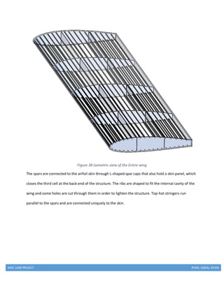
end](https://image.slidesharecdn.com/6e03d563-46c5-4e39-b180-83d24f29102e-170124015624/85/Report-Wing-Structure-Design-Spring-16-93-320.jpg)

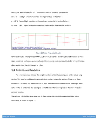
This document summarizes the wing design project for a Cessna 177 Cardinal aircraft. It describes using Xfoil software to analyze the NACA 2415 airfoil and generate aerodynamic data. Key points analyzed include wing loading during different flight conditions, maneuver loading during banked turns, and interpreting Xfoil output to create V-n diagrams showing stall curves. The document contains the project description, assumptions made, parameters chosen, and a Gantt chart showing the project timeline. Tables and figures are included to illustrate concepts and results.


![L3 - Aerodynamics [BB] for AGP Project Work](https://cdn.slidesharecdn.com/ss_thumbnails/l3-aerodynamicsbb-250321220306-5985ad4a-thumbnail.jpg?width=640&height=640&fit=bounds)
![[Sapienza] Development of the Flight Dynamics Model of a Flying Wing Aircraft](https://cdn.slidesharecdn.com/ss_thumbnails/355a5afb-e186-4fcb-b8a5-c15a5650ca6a-160412194308-thumbnail.jpg?width=640&height=640&fit=bounds)


