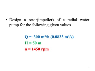
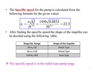
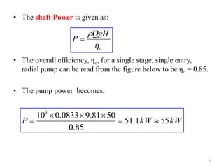
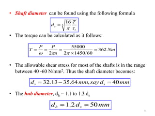
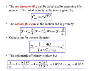
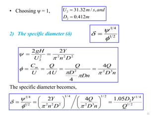
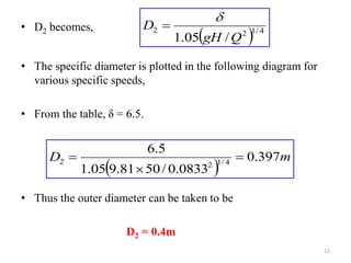
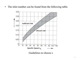
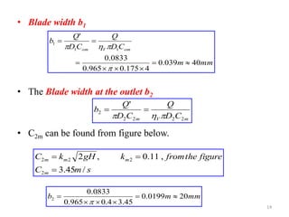
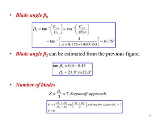
This document provides steps to design the impeller of a radial water pump. Key details include: - The specific speed is calculated to be 51.9, indicating a radial type impeller shape. - The pump power is calculated to be 55 kW. - Dimensions like the shaft diameter, eye diameter, and outer diameters are determined using formulas involving flow rate, head, speed and material properties. - Blade width, angles and number of blades are estimated from standard reference diagrams.

1. Radial Pump Impeller Design
(Example)
1

2. • Design a rotor(impeller) of a radial water
pump for the following given values
Q = 300 m3/h (0.0833 m3/s)
H = 50 m
n = 1450 rpm
2

3. • The Specific speed for the pump is calculated from the
following formula for the given values
• After finding the specific speed the shape of the impeller can
be decided using the following table.
 The specific speed is in the radial type pump range
3
.
22
50
0833
.
0
1450
4
3
4
3



H
Q
n
ns
Shape No. Range Shape of the Impeller
10<ns<50 Radial Type
50<ns<150 Mixed Type
150<Ns<400 Axial Type
3

4. • The shaft Power is given as:
• The overall efficiency, ηo, for a single stage, single entry,
radial pump can be read from the figure below to be ηo = 0.85.
• The pump power becomes,
o
QgH
P



kW
kW
P 55
1
.
51
85
.
0
50
81
.
9
0833
.
0
103






4

5. (Source: Centrifugal Pumps, Johann Friedrich Gülich, 2nd ed)
5

6. • Shaft diameter can be found using the following formula
• The torque can be calculated as it follows:
• The allowable shear stress for most of the shafts is in the range
between 40 -60 N/mm2. Thus the shaft diameter becomes:
• The hub diameter, dh = 1.1 to 1.3 ds
3
16
t
s
T
d



Nm
n
P
P
T 362
60
1450
2
55000
2








mm
d
say
mm
d s
s 40
,
64
.
35
13
.
32 


mm
d
d s
h 50
2
.
1 

6

7. • The eye diameter (D1) can be calculated by assuming inlet
number . The radial velocity at the inlet is given by:
• The volume flow rate at the suction end is given by:
• Calculating for the eye diameter,
• The volumetric efficiency is given by:
Y
Com 2


 
V
h
om
Q
Q
Where
d
D
C
Q




 '
,
4
' 2
2
1
965
.
0
,
,
0362
.
1
,
3
.
22
287
.
0
1
,
287
.
0
1
1
3
2
3
2





 V
s
V
or
n


2
1
4
h
V
om
d
C
Q
D 





7

8. • The inlet number can be found from the following table.
Guidelines to choose ε
8

9. • From the table,
• Thus,
• Another option to estimate the value of inlet number is to use
the formula by Pfleiderer,
• Thus, D1 becomes,
3
.
22
,
13
.
0
08
.
0 

 s
n
for

s
m
s
m
Com /
4
/
52
.
7
5
.
2 


3
2
2
10
).
3
5
.
1
( s
n




m
m
D 175
.
0
173
.
0
05
.
0
965
.
0
4
0833
.
0
4 2
1 







9

10. The outer diameter D2 can be calculated using:
1) The head coefficient (ψ)
The head coefficient for different type of pumps is given below.
2
2
2
U
gH


ψ Pump Type
0.7-1.3 Radial Impeller
0.25-0.7 Mixed-flow impeller
0.1-0.4 Axial Impeller

 gH
n
D
U
2
60
2
2 



gH
n
D
2
60
2 
10

11. • Choosing ψ = 1,
2) The specific diameter (δ)
The specific diameter becomes,
m
D
and
s
m
U
412
.
0
,
/
32
.
31
2
2


2
1
4
1


 
n
D
Q
Dn
D
Q
AU
Q
U
C
D
n
Y
U
gH
m
3
2
2
2
2
2
2
2
4
4
2
2












2
/
1
4
/
1
2
2
/
1
3
2
4
/
1
2
2
2
2
1
4
1
05
.
1
4
2
Q
Y
D
n
D
Q
D
n
Y




















11

12. • D2 becomes,
• The specific diameter is plotted in the following diagram for
various specific speeds,
• From the table, δ = 6.5.
• Thus the outer diameter can be taken to be
D2 = 0.4m
  4
/
1
2
2
/
05
.
1 Q
gH
D


 
m
D 397
.
0
0833
.
0
/
50
81
.
9
05
.
1
5
.
6
4
/
1
2
2 


12

13. Cordier Diagram 13

14. • Blade width b1
• The Blade width at the outlet b2
• C2m can be found from figure below.
mm
m
C
D
Q
C
D
Q
b
om
V
om
40
039
.
0
4
175
.
0
965
.
0
0833
.
0
'
1
1
1












m
V
m C
D
Q
C
D
Q
b
2
2
2
2
2
'





s
m
C
figure
the
from
k
gH
k
C
m
m
m
m
/
45
.
3
,
11
.
0
,
2
2
2
2
2



mm
m
b 20
0199
.
0
45
.
3
4
.
0
965
.
0
0833
.
0
2 






14

15. 15

16. • Blade angle β0
• Blade angle β2 can be estimated from the previous figure.
• Number of blades
o
om
om
n
D
C
U
C
75
.
16
60
/
1450
175
.
0
4
tan
tan
tan
1
1
1
1
1
0


































o
o
to 3
.
23
8
.
21
43
.
0
4
.
0
tan
2
2





approach
Stepanoff
Z ,
7
3
2



6
7
,
2
sin 2
1
1
2
2
1







 



Z
k
of
value
the
taking
D
D
D
D
k
Z


16