Python Data Cleaning Cookbook Second Edition Michael Walker
Python Data Cleaning Cookbook Second Edition Michael Walker
Python Data Cleaning Cookbook Second Edition Michael Walker
Python Data Cleaning Cookbook Second Edition Michael Walker
Python Data Cleaning Cookbook Second Edition Michael Walker
1.
Python Data CleaningCookbook Second Edition
Michael Walker download
https://ebookbell.com/product/python-data-cleaning-cookbook-
second-edition-michael-walker-56138680
Explore and download more ebooks at ebookbell.com
2.
Here are somerecommended products that we believe you will be
interested in. You can click the link to download.
Python Data Cleaning Cookbook Second Edition Converted Michael Walker
https://ebookbell.com/product/python-data-cleaning-cookbook-second-
edition-converted-michael-walker-56696340
Python Data Cleaning Cookbook Early Access 2nd Michael Walker
https://ebookbell.com/product/python-data-cleaning-cookbook-early-
access-2nd-michael-walker-53625900
Python Data Cleaning Cookbook Modern Techniques And Python Tools To
Detect And Remove Dirty Data And Extract Key Insights Walker
https://ebookbell.com/product/python-data-cleaning-cookbook-modern-
techniques-and-python-tools-to-detect-and-remove-dirty-data-and-
extract-key-insights-walker-56138740
Python Data Cleaning Cookbook Modern Techniques And Python Tools To
Detect And Remove Dirty Data And Extract Key Insights Michael Walker
https://ebookbell.com/product/python-data-cleaning-cookbook-modern-
techniques-and-python-tools-to-detect-and-remove-dirty-data-and-
extract-key-insights-michael-walker-49848532
3.
Python Data CleaningCookbook Michael Walker
https://ebookbell.com/product/python-data-cleaning-cookbook-michael-
walker-170777174
Python Data Cleaning And Preparation Best Practices Maria Zervou
https://ebookbell.com/product/python-data-cleaning-and-preparation-
best-practices-maria-zervou-156869314
Python Data Cleaning And Preparation Best Practices Maria Zervou
https://ebookbell.com/product/python-data-cleaning-and-preparation-
best-practices-maria-zervou-63298198
Python Data Cleaning How To Describe Data In Detail Identify Solve
Issues Using Commonly Used Techniques And Tips And Tricks Ochoa
https://ebookbell.com/product/python-data-cleaning-how-to-describe-
data-in-detail-identify-solve-issues-using-commonly-used-techniques-
and-tips-and-tricks-ochoa-232141092
Practical Python Data Wrangling And Data Quality Getting Started With
Reading Cleaning And Analyzing Data 1st Edition Susan E Mcgregor
https://ebookbell.com/product/practical-python-data-wrangling-and-
data-quality-getting-started-with-reading-cleaning-and-analyzing-
data-1st-edition-susan-e-mcgregor-36558596
Table of Contents
1.Python Data Cleaning Cookbook, Second Edition: Detect and remove
dirty data and extract key insights with pandas, machine learning and
ChatGPT, Spark, and more
2. 1 Anticipating Data Cleaning Issues when Importing Tabular Data into
Pandas
I. Join our book community on Discord
II. Importing CSV files
i. Getting ready
ii. How to do it…
iii. How it works...
iv. There’s more...
v. See also
III. Importing Excel files
i. Getting ready
ii. How to do it…
iii. How it works…
iv. There’s more…
v. See also
IV. Importing data from SQL databases
i. Getting ready
ii. How to do it...
iii. How it works…
iv. There’s more…
v. See also
V. Importing SPSS, Stata, and SAS data
i. Getting ready
ii. How to do it...
iii. How it works...
iv. There’s more…
v. See also
VI. Importing R data
i. Getting ready
ii. How to do it…
8.
iii. How itworks…
iv. There’s more…
v. See also
VII. Persisting tabular data
i. Getting ready
ii. How to do it…
iii. How it works...
iv. There’s more...
3. 2 Anticipating Data Cleaning Issues when Working with HTML, JSON,
and Spark Data
I. Join our book community on Discord
II. Importing simple JSON data
i. Getting ready…
ii. How to do it…
iii. How it works…
iv. There’s more…
III. Importing more complicated JSON data from an API
i. Getting ready…
ii. How to do it...
iii. How it works…
iv. There’s more…
v. See also
IV. Importing data from web pages
i. Getting ready...
ii. How to do it…
iii. How it works…
iv. There’s more…
V. Working with Spark data
i. Getting ready...
ii. How it works...
iii. There’s more...
VI. Persisting JSON data
i. Getting ready…
ii. How to do it...
iii. How it works…
iv. There’s more…
4. 3 Taking the Measure of Your Data
9.
I. Join ourbook community on Discord
II. Getting a first look at your data
i. Getting ready…
ii. How to do it...
iii. How it works…
iv. There’s more...
v. See also
III. Selecting and organizing columns
i. Getting Ready…
ii. How to do it…
iii. How it works…
iv. There’s more…
v. See also
IV. Selecting rows
i. Getting ready...
ii. How to do it...
iii. How it works…
iv. There’s more…
v. See also
V. Generating frequencies for categorical variables
i. Getting ready…
ii. How to do it…
iii. How it works…
iv. There’s more…
VI. Generating summary statistics for continuous variables
i. Getting ready…
ii. How to do it…
iii. How it works…
iv. See also
VII. Using generative AI to view our data
i. Getting ready…
ii. How to do it…
iii. How it works…
iv. See also
5. 4 Identifying Missing Values and Outliers in Subsets of Data
I. Join our book community on Discord
II. Finding missing values
10.
i. Getting ready
ii.How to do it…
iii. How it works...
iv. See also
III. Identifying outliers with one variable
i. Getting ready
ii. How to do it...
iii. How it works…
iv. There’s more…
v. See also
IV. Identifying outliers and unexpected values in bivariate relationships
i. Getting ready
ii. How to do it...
iii. How it works…
iv. There’s more…
v. See also
V. Using subsetting to examine logical inconsistencies in variable
relationships
i. Getting ready
ii. How to do it…
iii. How it works…
iv. See also
VI. Using linear regression to identify data points with significant
influence
i. Getting ready
ii. How to do it…
iii. How it works...
iv. There’s more…
VII. Using K-nearest neighbor to find outliers
i. Getting ready
ii. How to do it…
iii. How it works...
iv. There’s more...
v. See also
VIII. Using Isolation Forest to find anomalies
i. Getting ready
ii. How to do it...
11.
iii. How itworks…
iv. There’s more…
v. See also
6. 5 Using Visualizations for the Identification of Unexpected Values
I. Join our book community on Discord
II. Using histograms to examine the distribution of continuous
variables
i. Getting ready
ii. How to do it…
iii. How it works…
iv. There’s more...
III. Using boxplots to identify outliers for continuous variables
i. Getting ready
ii. How to do it…
iii. How it works...
iv. There’s more...
v. See also
IV. Using grouped boxplots to uncover unexpected values in a
particular group
i. Getting ready
ii. How to do it...
iii. How it works...
iv. There’s more…
v. See also
V. Examining both distribution shape and outliers with violin plots
i. Getting ready
ii. How to do it…
iii. How it works…
iv. There’s more…
v. See also
VI. Using scatter plots to view bivariate relationships
i. Getting ready
ii. How to do it...
iii. How it works…
iv. There’s more...
v. See also
VII. Using line plots to examine trends in continuous variables
12.
i. Getting ready
ii.How to do it…
iii. How it works...
iv. There’s more…
v. See also
VIII. Generating a heat map based on a correlation matrix
i. Getting ready
ii. How to do it…
iii. How it works…
iv. There’s more…
v. See also
13.
Python Data CleaningCookbook,
Second Edition: Detect and remove
dirty data and extract key insights
with pandas, machine learning and
ChatGPT, Spark, and more
Welcome to Packt Early Access. We’re giving you an exclusive preview of
this book before it goes on sale. It can take many months to write a book, but
our authors have cutting-edge information to share with you today. Early
Access gives you an insight into the latest developments by making chapter
drafts available. The chapters may be a little rough around the edges right
now, but our authors will update them over time.You can dip in and out
of this book or follow along from start to finish; Early Access is designed to
be flexible. We hope you enjoy getting to know more about the process of
writing a Packt book.
1. Chapter 1: Anticipating Data Cleaning Issues when Importing Tabular
Data into Pandas
2. Chapter 2: Anticipating Data Cleaning Issues when Working with
HTML, JSON, and Spark Data
3. Chapter 3: Taking the Measure of Your Data
4. Chapter 4: Identifying Missing Values and Outliers in Subsets of Data
5. Chapter 5: Using Visualizations for the Identification of Unexpected
Values
6. Chapter 6: Cleaning and Exploring Data with Series Operations
7. Chapter 7: Working with Missing Data
8. Chapter 8: Fixing Messy Data When Aggregating
9. Chapter 9: Addressing Data Issues When Combining Data Frames
10. Chapter 10: Tidying and Reshaping Data
11. Chapter 11: Automate Data Cleaning with User-Defined Functions and
Join our bookcommunity on Discord
https://discord.gg/28TbhyuH
Scientific distributions of Python (Anaconda, WinPython, Canopy, and so
on) provide analysts with an impressive range of data manipulation,
exploration, and visualization tools. One important tool is pandas. Developed
by Wes McKinney in 2008, but really gaining in popularity after 2012,
pandas is now an essential library for data analysis in Python. We work with
pandas extensively in this book, along with popular packages such as numpy ,
matplotlib , and scipy .A key pandas object is the DataFrame, which
represents data as a tabular structure, with rows and columns. In this way, it
is similar to the other data stores we discuss in this chapter. However, a
pandas DataFrame also has indexing functionality that makes selecting,
combining, and transforming data relatively straightforward, as the recipes in
this book will demonstrate.Before we can make use of this great
functionality, we have to get our data into pandas. Data comes to us in a wide
variety of formats: as CSV or Excel files, as tables from SQL databases, from
statistical analysis packages such as SPSS, Stata, SAS, or R, from non-tabular
sources such as JSON, and from web pages.We examine tools for importing
tabular data in this recipe. Specifically, we cover the following topics:
Importing CSV files
Importing Excel files
Importing data from SQL databases
17.
Importing SPSS, Stata,and SAS data
Importing R data
Persisting tabular data
Importing CSV files
The read_csv method of the pandas library can be used to read a file with
comma separated values (CSV) and load it into memory as a pandas
DataFrame. In this recipe, we read a CSV file and address some common
issues: creating column names that make sense to us, parsing dates, and
dropping rows with critical missing data.Raw data is often stored as CSV
files. These files have a carriage return at the end of each line of data to
demarcate a row, and a comma between each data value to delineate columns.
Something other than a comma can be used as the delimiter, such as a tab.
Quotation marks may be placed around values, which can be helpful when
the delimiter occurs naturally within certain values, which sometimes
happens with commas.All data in a CSV file are characters, regardless of the
logical data type. This is why it is easy to view a CSV file, presuming it is not
too large, in a text editor. The pandas read_csv method will make an
educated guess about the data type of each column, but you will need to help
it along to ensure that these guesses are on the mark.
Getting ready
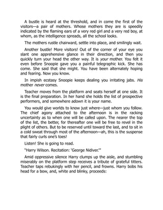
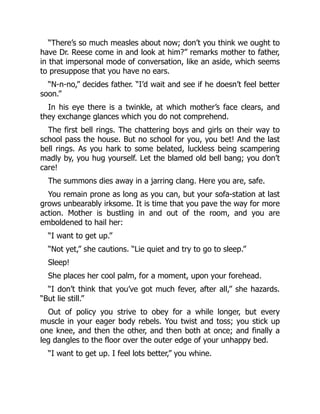
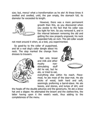
Create a folder for this chapter and create a new Python script or Jupyter
Notebook file in that folder. Create a data subfolder and place the
landtempssample.csv file in that subfolder. Alternatively, you could
retrieve all of the files from the GitHub repository. Here is a screenshot of the
beginning of the CSV file:
18.
Figure 1.1: LandTemperatures Data
Note
This dataset, taken from the Global Historical Climatology
Network integrated database, is made available for public use by
the United States National Oceanic and Atmospheric
Administration at https://www.ncdc.noaa.gov/data-access/land-
based-station-data/land-based-datasets/global-historical-
climatology-network-monthly-version-4. This is just a 100,000-row
sample of the full dataset, which is also available in the repository.
How to do it…
We will import a CSV file into pandas, taking advantage of some very useful
read_csv options:
1. Import the pandas library and set up the environment to make viewing
the output easier:
import pandas as pd
pd.options.display.float_format = '{:,.2f}'.format
19.
pd.set_option('display.width', 85)
pd.set_option('display.max_columns', 8)
1.Read the data file, set new names for the headings, and parse the date
column.
Pass an argument of 1 to the skiprows parameter to skip the first row, pass
a list of columns to parse_dates to create a pandas datetime column from
those columns, and set low_memory to False to reduce the usage of memory
during the import process:
landtemps = pd.read_csv('data/landtempssample.csv',
... names=['stationid','year','month','avgtemp','latitude',
... 'longitude','elevation','station','countryid','country
'],
... skiprows=1,
... parse_dates=[['month','year']],
... low_memory=False)
>>> type(landtemps)
<class 'pandas.core.frame.DataFrame'>
Note
We have to use skiprows because we are passing a list of column
names to read_csv . If we use the column names in the CSV file
we do not need to specify values for either names or skiprows .
1. Get a quick glimpse of the data.
View the first few rows. Show the data type for all columns, as well as
the number of rows and columns:
>>> landtemps.head(7)
month_year stationid ... countryid
0 2000-04-01 USS0010K01S ... US
1 1940-05-01 CI000085406 ... CI
2 2013-12-01 USC00036376 ... US
3 1963-02-01 ASN00024002 ... AS
4 2001-11-01 ASN00028007 ... AS
5 1991-04-01 USW00024151 ... US
6 1993-12-01 RSM00022641 ... RS
country
20.
0 United States
1Chile
2 United States
3 Australia
4 Australia
5 United States
6 Russia
[7 rows x 9 columns]
>>> landtemps.dtypes
month_year datetime64[ns]
stationid object
avgtemp float64
latitude float64
longitude float64
elevation float64
station object
countryid object
country object
dtype: object
>>> landtemps.shape
(100000, 9)
1. Give the date column a better name and view the summary statistics for
average monthly temperature:
>>> landtemps.rename(columns={'month_year':'measuredate'}, inpla
ce=True)
>>> landtemps.dtypes
measuredate datetime64[ns]
stationid object
avgtemp float64
latitude float64
longitude float64
elevation float64
station object
countryid object
country object
dtype: object
>>> landtemps.avgtemp.describe()
count 85,554.00
mean 10.92
21.
std 11.52
min -70.70
25%3.46
50% 12.22
75% 19.57
max 39.95
Name: avgtemp, dtype: float64
1. Look for missing values for each column.
Use isnull , which returns True for each value that is missing for each
column, and False when not missing. Chain this with sum to count the
missings for each column. (When working with Boolean values, sum treats
True as 1 and False as 0 . I will discuss method chaining in the There’s
more... section of this recipe):
>>> landtemps.isnull().sum()
measuredate 0
stationid 0
avgtemp 14446
latitude 0
longitude 0
elevation 0
station 0
countryid 0
country 5
dtype: int64
1. Remove rows with missing data for avgtemp .
Use the subset parameter to tell dropna to drop rows when avgtemp is
missing. Set inplace to True . Leaving inplace at its default value of
False would display the DataFrame, but the changes we have made would
not be retained. Use the shape attribute of the DataFrame to get the number
of rows and columns:
>>> landtemps.dropna(subset=['avgtemp'], inplace=True)
>>> landtemps.shape
(85554, 9)
That’s it! Importing CSV files into pandas is as simple as that.
22.
How it works...
Almostall of the recipes in this book use the pandas library. We refer to it
as pd to make it easier to reference later. This is customary. We also use
float_format to display float values in a readable way and set_option to
make the terminal output wide enough to accommodate the number of
variables.Much of the work is done by the first line in step 2. We use
read_csv to load a pandas DataFrame in memory and call it landtemps . In
addition to passing a filename, we set the names parameter to a list of our
preferred column headings. We also tell read_csv to skip the first row, by
setting skiprows to 1, since the original column headings are in the first row
of the CSV file. If we do not tell it to skip the first row, read_csv will treat
the header row in the file as actual data. read_csv also solves a date
conversion issue for us. We use the parse_dates parameter to ask it to
convert the month and year columns to a date value.Step 3 runs through a
few standard data checks. We use head(7) to print out all columns for the
first 7 rows. We use the dtypes attribute of the data frame to show the data
type of all columns. Each column has the expected data type. In pandas,
character data has the object data type, a data type that allows for mixed
values. shape returns a tuple, whose first element is the number of rows in
the data frame (100,000 in this case) and whose second element is the
number of columns (9).When we used read_csv to parse the month and
year columns, it gave the resulting column the name month_year . We use
the rename method in step 4 to give that column a better name. We need to
specify inplace=True to replace the old column name with the new column
name in memory. The describe method provides summary statistics on the
avgtemp column.Notice that the count for avgtemp indicates that there are
85,554 rows that have valid values for avgtemp . This is out of 100,000 rows
for the whole DataFrame, as provided by the shape attribute. The listing of
missing values for each column in step 5 ( landtemps.isnull().sum() )
confirms this: 100,000 – 85,554 = 14,446.Step 6 drops all rows where
avgtemp is NaN . (The NaN value, not a number, is the pandas representation
of missing values.) subset is used to indicate which column to check for
missings. The shape attribute for landtemps now indicates that there are
85,554 rows, which is what we would expect given the previous count from
describe .
23.
There’s more...
If thefile you are reading uses a delimiter other than a comma, such as a tab,
this can be specified in the sep parameter of read_csv . When creating the
pandas DataFrame, an index was also created. The numbers to the far left of
the output when head and sample were run are index values. Any number
of rows can be specified for head or sample . The default value is 5 .Setting
low_memory to False causes read_csv to parse data in chunks. This is
easier on systems with lower memory when working with larger files.
However, the full DataFrame will still be loaded into memory once
read_csv completes successfully.The landtemps.isnull().sum()
statement is an example of chaining methods. First, isnull returns a
DataFrame of True and False values, resulting from testing whether each
column value is null . sum takes that DataFrame and sums the True values
for each column, interpreting the True values as 1 and the False values as
0 . We would have obtained the same result if we had used the following two
steps:
>>> checknull = landtemps.isnull()
>>> checknull.sum()
There is no hard and fast rule for when to chain methods and when not to do
so. I find it helpful to chain when I really think of something I am doing as
being a single step, but only two or more steps, mechanically speaking.
Chaining also has the side benefit of not creating extra objects that I might
not need.The dataset used in this recipe is just a sample from the full land
temperatures database with almost 17 million records. You can run the larger
file if your machine can handle it, with the following code:
>>> landtemps = pd.read_csv('data/landtemps.zip',
... compression='zip', names=['stationid','year',
... 'month','avgtemp','latitude','longitude',
... 'elevation','station','countryid','country'],
... skiprows=1,
... parse_dates=[['month','year']],
... low_memory=False)
read_csv can read a compressed ZIP file. We get it to do this by passing the
name of the ZIP file and the type of compression.
24.
See also
Subsequent recipesin this chapter, and in other chapters, set indexes to
improve navigation over rows and merging.A significant amount of
reshaping of the Global Historical Climatology Network raw data was done
before using it in this recipe. We demonstrate this in Chapter 8, Tidying and
Reshaping Data.
Importing Excel files
The read_excel method of the pandas library can be used to import data
from an Excel file and load it into memory as a pandas DataFrame. In this
recipe, we import an Excel file and handle some common issues when
working with Excel files: extraneous header and footer information, selecting
specific columns, removing rows with no data, and connecting to particular
sheets.Despite the tabular structure of Excel, which invites the organization
of data into rows and columns, spreadsheets are not datasets and do not
require people to store data in that way. Even when some data conforms with
those expectations, there is often additional information in rows or columns
before or after the data to be imported. Data types are not always as clear as
they are to the person who created the spreadsheet. This will be all too
familiar to anyone who has ever battled with importing leading zeros.
Moreover, Excel does not insist that all data in a column be of the same type,
or that column headings be appropriate for use with a programming language
such as Python.Fortunately, read_excel has a number of options for
handling messiness in Excel data. These options make it relatively easy to
skip rows and select particular columns, and to pull data from a particular
sheet or sheets.
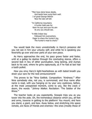
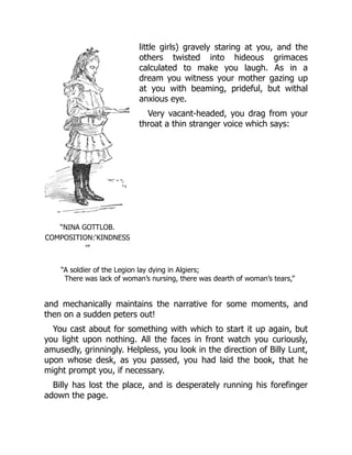
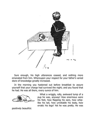
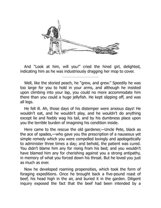
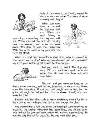
Getting ready
You can download the GDPpercapita.xlsx file, as well as the code for this
recipe, from the GitHub repository for this book. The code assumes that the
Excel file is in a data subfolder. Here is a view of the beginning of the file:
25.
Figure 1.2: Viewof the dataset
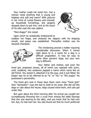
And here is a view of the end of the file:
Figure 1.3: View of the dataset
Note
This dataset, from the Organisation for Economic Co-operation and
Development, is available for public use at https://stats.oecd.org/.
How to do it…
We import an Excel file into pandas and do some initial data cleaning:
1. Import the pandas library:
>>> import pandas as pd
1. Read the Excel per capita GDP data.
Select the sheet with the data we need, but skip the columns and rows that we
do not want. Use the sheet_name parameter to specify the sheet. Set
skiprows to 4 and skipfooter to 1 to skip the first four rows (the first
row is hidden) and the last row. We provide values for usecols to get data
from column A and columns C through T (column B is blank). Use head
26.
to view thefirst few rows:
>>> percapitaGDP = pd.read_excel("data/GDPpercapita.xlsx",
... sheet_name="OECD.Stat export",
... skiprows=4,
... skipfooter=1,
... usecols="A,C:T")
>>> percapitaGDP.head()
Year 2001 2017 2018
0 Metropolitan areas NaN NaN NaN
1 AUS: Australia
2 AUS01: Greater Sydney 43313 50578 49860
3 AUS02: Greater Melbourne 40125 43025 42674
4 AUS03: Greater Brisbane 37580 46876 46640
[5 rows x 19 columns]
1. Use the info method of the data frame to view data types and the
non-null count:
>>> percapitaGDP.info()
<class 'pandas.core.frame.DataFrame'>
RangeIndex: 702 entries, 0 to 701
Data columns (total 19 columns):
# Column Non-Null Count Dtype
--- ------ -------------- -----
0 Year 702 non-null object
1 2001 701 non-null object
2 2002 701 non-null object
3 2003 701 non-null object
4 2004 701 non-null object
5 2005 701 non-null object
6 2006 701 non-null object
7 2007 701 non-null object
8 2008 701 non-null object
9 2009 701 non-null object
10 2010 701 non-null object
11 2011 701 non-null object
12 2012 701 non-null object
13 2013 701 non-null object
14 2014 701 non-null object
15 2015 701 non-null object
16 2016 701 non-null object
17 2017 701 non-null object
18 2018 701 non-null object
dtypes: object(19)
27.
memory usage: 104.3+KB
1. Rename the Year column to metro and remove the leading spaces.
Give an appropriate name to the metropolitan area column. There are extra
spaces before the metro values in some cases, and extra spaces after the metro
values in others. We can test for leading spaces with startswith(‘ ‘) and then
use any to establish whether there are one or more occasions when the first
character is blank. We can use endswith(‘ ‘) to examine trailing spaces. We
use strip to remove both leading and trailing spaces. When we test for trailing
spaces again we see that there are none:
>>> percapitaGDP.rename(columns={'Year':'metro'}, inplace=True)
>>> percapitaGDP.metro.str.startswith(' ').any()
True
>>> percapitaGDP.metro.str.endswith(' ').any()
True
>>> percapitaGDP.metro = percapitaGDP.metro.str.strip()
percapitaGDP.metro.str.endswith(' ').any()
False
1. Convert the data columns to numeric.
Iterate over all of the GDP year columns (2001-2018) and convert the data
type from object to float . Coerce the conversion even when there is
character data – the .. in this example. We want character values in those
columns to become missing, which is what happens. Rename the year
columns to better reflect the data in those columns:
>>> for col in percapitaGDP.columns[1:]:
... percapitaGDP[col] = pd.to_numeric(percapitaGDP[col],
... errors='coerce')
... percapitaGDP.rename(columns={col:'pcGDP'+col},
... inplace=True)
...
metro pcGDP2001 ...
0 Metropolitan areas NaN ...
1 AUS: Australia NaN ...
28.
2 AUS01:Greater Sydney43313 ...
3 AUS02: Greater Melbourne 40125 ...
4 AUS03: Greater Brisbane 37580 ...
pcGDP2017 pcGDP2018
0 NaN NaN
1 NaN NaN
2 50578 49860
3 43025 42674
4 46876 46640
[5 rows x 19 columns]
>>> percapitaGDP.dtypes
metro object
pcGDP2001 float64
pcGDP2002 float64
abbreviated to save space
pcGDP2017 float64
pcGDP2018 float64
dtype: object
1. Use the describe method to generate summary statistics for all
numeric data in the data frame:
>>> percapitaGDP.describe()
pcGDP2001 pcGDP2002 pcGDP2017 pcGDP2018
count 424 440 445 441
mean 41264 41015 47489 48033
std 11878 12537 15464 15720
min 10988 11435 2745 2832
25% 33139 32636 37316 37908
50% 39544 39684 45385 46057
75% 47972 48611 56023 56638
max 91488 93566 122242 127468
[8 rows x 18 columns]
1. Remove rows where all of the per capita GDP values are missing.
Use the subset parameter of dropna to inspect all columns, starting with
the second column (it is zero-based) through the last column. Use how to
specify that we want to drop rows only if all of the columns specified in
subset are missing. Use shape to show the number of rows and columns in
the resulting DataFrame:
>>> percapitaGDP.dropna(subset=percapitaGDP.columns[1:], how="al
l", inplace=True)
29.
>>> percapitaGDP.describe()
pcGDP2001 pcGDP2002pcGDP2017 pcGDP2018
count 424 440 445 441
mean 41264 41015 47489 48033
std 11878 12537 15464 15720
min 10988 11435 2745 2832
25% 33139 32636 37316 37908
50% 39544 39684 45385 46057
75% 47972 48611 56023 56638
max 91488 93566 122242 127468
[8 rows x 18 columns]
>>> percapitaGDP.head()
metro pcGDP2001 pcGDP2002
2 AUS01: Greater Sydney 43313 44008
3 AUS02: Greater Melbourne 40125 40894
4 AUS03:Greater Brisbane 37580 37564
5 AUS04: Greater Perth 45713 47371
6 AUS05: Greater Adelaide 36505 37194
... pcGDP2016 pcGDP2017 pcGDP2018
2 ... 50519 50578 49860
3 ... 42671 43025 42674
4 ... 45723 46876 46640
5 ... 66032 66424 70390
6 ... 39737 40115 39924
[5 rows x 19 columns]
>>> percapitaGDP.shape
(480, 19)
1. Set the index for the DataFrame using the metropolitan area column.
Confirm that there are 480 valid values for metro and that there are 480
unique values, before setting the index:
>>> percapitaGDP.metro.count()
480
>>> percapitaGDP.metro.nunique()
480
>>> percapitaGDP.set_index('metro', inplace=True)
>>> percapitaGDP.head()
pcGDP2001 ... pcGDP2018
metro ...
30.
AUS01: Greater Sydney43313 ... 49860
AUS02: Greater Melbourne 40125 ... 42674
AUS03: Greater Brisbane 37580 ... 46640
AUS04: Greater Perth 45713 ... 70390
AUS05: Greater Adelaide 36505 ... 39924
[5 rows x 18 columns]
>>> percapitaGDP.loc['AUS02: Greater Melbourne']
pcGDP2001 40125
pcGDP2002 40894
...
pcGDP2017 43025
pcGDP2018 42674
Name: AUS02: Greater Melbourne, dtype: float64
We have now imported the Excel data into a pandas data frame and cleaned
up some of the messiness in the spreadsheet.
How it works…
We mostly manage to get the data we want in step 2 by skipping rows and
columns we do not want, but there are still a number of issues: read_excel
interprets all of the GDP data as character data, many rows are loaded with
no useful data, and the column names do not represent the data well. In
addition, the metropolitan area column might be useful as an index, but there
are leading and trailing blanks and there may be missing or duplicated
values. read_excel interprets Year as the column name for the metropolitan
area data because it looks for a header above the data for that Excel column
and finds Year there. We rename that column metro in step 4. We also use
strip to fix the problem with leading and trailing blanks. If there had only
been leading blanks, we could have used lstrip , or rstrip if there had
only been trailing blanks. It is a good idea to assume that there might be
leading or trailing blanks in any character data and clean that data shortly
after the initial import.The spreadsheet authors used .. to represent missing
data. Since this is actually valid character data, those columns get the object
data type (that is how pandas treats columns with character or mixed data).
We coerce a conversion to numeric in step 5. This also results in the original
values of .. being replaced with NaN (not a number), pandas missing values
for numbers. This is what we want.We can fix all of the per capita GDP
columns with just a few lines because pandas makes it easy to iterate over the
31.
columns of aDataFrame. By specifying [1:] , we iterate from the second
column to the last column. We can then change those columns to numeric
and rename them to something more appropriate.There are several reasons
why it is a good idea to clean up the column headings for the annual GDP
columns: it helps us to remember what the data actually is; if we merge it
with other data by metropolitan area, we will not have to worry about
conflicting variable names; and we can use attribute access to work with
pandas series based on those columns, which I will discuss in more detail in
the There’s more… section of this recipe. describe in step 6 shows us that
fewer than 500 rows have valid data for per capita GDP. When we drop all
rows that have missing values for all per capita GDP columns in step 7, we
end up with 480 rows in the DataFrame.
There’s more…
Once we have a pandas DataFrame, we have the ability to treat columns as
more than just columns. We can use attribute access (such as
percapitaGPA.metro ) or bracket notation ( percapitaGPA[‘metro’] ) to get
the functionality of a pandas data series. Either method makes it possible to
use data series string inspecting methods such as str.startswith , and
counting methods such as nunique . Note that the original column names of
20## did not allow for attribute access because they started with a number,
so percapitaGDP.pcGDP2001.count() works, but
percapitaGDP.2001.count() returns a syntax error because 2001 is not a
valid Python identifier (since it starts with a number).pandas is rich with
features for string manipulation and for data series operations. We will try
many of them out in subsequent recipes. This recipe showed those I find most
useful when importing Excel data.
See also
There are good reasons to consider reshaping this data. Instead of 18 columns
of GDP per capita data for each metropolitan area, we should have 18 rows of
data for each metropolitan area, with columns for year and GDP per capita.
Recipes for reshaping data can be found in Chapter 9, Tidying and Reshaping
Data.
32.
Importing data fromSQL databases
In this recipe, we will use pymssql and mysql apis to read data from
Microsoft SQL Server and MySQL (now owned by Oracle) databases,
respectively. Data from sources such as these tends to be well structured
since it is designed to facilitate simultaneous transactions by members of
organizations, and those who interact with them. Each transaction is also
likely related to some other organizational transaction.This means that
although data tables from enterprise systems are more reliably structured than
data from CSV files and Excel files, their logic is less likely to be self-
contained. You need to know how the data from one table relates to data from
another table to understand its full meaning. These relationships need to be
preserved, including the integrity of primary and foreign keys, when pulling
data. Moreover, well-structured data tables are not necessarily uncomplicated
data tables. There are often sophisticated coding schemes that determine data
values, and these coding schemes can change over time. For example, codes
for staff ethnicity at a retail store chain might be different in 1998 than they
are in 2020. Similarly, frequently there are codes for missing values, such as
99999, that pandas will understand as valid values.Since much of this logic is
business logic, and implemented in stored procedures or other applications, it
is lost when pulled out of this larger system. Some of what is lost will
eventually have to be reconstructed when preparing data for analysis. This
almost always involves combining data from multiple tables, so it is
important to preserve the ability to do that. But it also may involve adding
some of the coding logic back after loading the SQL table into a pandas
DataFrame. We explore how to do that in this recipe.
Getting ready
This recipe assumes you have pymssql and mysql apis installed. If you do
not, it is relatively straightforward to install them with pip . From the
terminal, or powershell (in Windows), enter pip install pymssql or
pip install mysql-connector-python .
Note
The dataset used in this recipe is available for public use at
33.
https://archive.ics.uci.edu/ml/machine-learning-databases/00320/.
How to doit...
We import SQL Server and MySQL data tables into a pandas data frame as
follows:
1. Import pandas , numpy , pymssql , and mysql .
This step assumes that you have installed pymssql and mysql apis :
>>> import pandas as pd
>>> import numpy as np
>>> import pymssql
>>> import mysql.connector
1. Use pymssql api and read_sql to retrieve and load data from a SQL
Server instance.
Select the columns we want from the SQL Server data and use SQL aliases to
improve column names (for example, fedu AS fathereducation ). Create a
connection to the SQL Server data by passing database credentials to the
pymssql connect function. Create a pandas data frame by passing the
select statement and connection object to read_sql . Close the
connection to return it to the pool on the server:
>>> sqlselect = "SELECT studentid, school, sex, age, famsize,
... medu AS mothereducation, fedu AS fathereducation,
... traveltime, studytime, failures, famrel, freetime,
... goout, g1 AS gradeperiod1, g2 AS gradeperiod2,
... g3 AS gradeperiod3 From studentmath"
>>>
>>> server = "pdcc.c9sqqzd5fulv.us-west-2.rds.amazonaws.com"
>>> user = "pdccuser"
>>> password = "pdccpass"
>>> database = "pdcctest"
>>>
>>> conn = pymssql.connect(server=server,
... user=user, password=password, database=database)
>>>
>>> studentmath = pd.read_sql(sqlselect,conn)
>>> conn.close()
34.
1. Check thedata types and the first few rows:
>>> studentmath.dtypes
studentid object
school object
sex object
age int64
famsize object
mothereducation int64
fathereducation int64
traveltime int64
studytime int64
failures int64
famrel int64
freetime int64
goout int64
gradeperiod1 int64
gradeperiod2 int64
gradeperiod3 int64
dtype: object
>>> studentmath.head()
studentid school ... gradeperiod2 gradeperiod3
0 001 GP ... 6 6
1 002 GP ... 5 6
2 003 GP ... 8 10
3 004 GP ... 14 15
4 005 GP ... 10 10
[5 rows x 16 columns]
1. (Alternative) Use the mysql connector and read_sql to get data from
MySQL.
Create a connection to the mysql data and pass that connection to read_sql
to retrieve the data and load it into a pandas data frame. (The same data file
on student math scores was uploaded to SQL Server and MySQL, so we can
use the same SQL select statement we used in the previous step.):
>>> host = "pdccmysql.c9sqqzd5fulv.us-west-2.rds.amazonaws.com"
>>> user = "pdccuser"
>>> password = "pdccpass"
>>> database = "pdccschema"
>>> connmysql = mysql.connector.connect(host=host,
35.
... database=database,user=user,password=password)
>>> studentmath= pd.read_sql(sqlselect,connmysql)
>>> connmysql.close()
1. Rearrange the columns, set an index, and check for missing values.
Move the grade data to the left of the DataFrame, just after studentid . Also
move the freetime column to the right after traveltime and studytime .
Confirm that each row has an ID and that the IDs are unique, and set
studentid as the index:
>>> newcolorder = ['studentid', 'gradeperiod1',
... 'gradeperiod2','gradeperiod3', 'school',
... 'sex', 'age', 'famsize','mothereducation',
... 'fathereducation', 'traveltime',
... 'studytime', 'freetime', 'failures',
... 'famrel','goout']
>>> studentmath = studentmath[newcolorder]
>>> studentmath.studentid.count()
395
>>> studentmath.studentid.nunique()
395
>>> studentmath.set_index('studentid', inplace=True)
1. Use the data frame’s count function to check for missing values:
>>> studentmath.count()
gradeperiod1 395
gradeperiod2 395
gradeperiod3 395
school 395
sex 395
age 395
famsize 395
mothereducation 395
fathereducation 395
traveltime 395
studytime 395
freetime 395
failures 395
famrel 395
36.
goout 395
dtype: int64
1.Replace coded data values with more informative values.
Create a dictionary with the replacement values for the columns, and then use
replace to set those values:
>>> setvalues=
... {"famrel":{1:"1:very bad",2:"2:bad",
... 3:"3:neutral",4:"4:good",5:"5:excellent"},
... "freetime":{1:"1:very low",2:"2:low",
... 3:"3:neutral",4:"4:high",5:"5:very high"},
... "goout":{1:"1:very low",2:"2:low",3:"3:neutral",
... 4:"4:high",5:"5:very high"},
... "mothereducation":{0:np.nan,1:"1:k-4",2:"2:5-9",
... 3:"3:secondary ed",4:"4:higher ed"},
... "fathereducation":{0:np.nan,1:"1:k-4",2:"2:5-9",
... 3:"3:secondary ed",4:"4:higher ed"}}
>>> studentmath.replace(setvalues, inplace=True)
1. Change the type for columns with the changed data to category .
Check any changes in memory usage:
>>> setvalueskeys = [k for k in setvalues]
>>> studentmath[setvalueskeys].memory_usage(index=False)
famrel 3160
freetime 3160
goout 3160
mothereducation 3160
fathereducation 3160
dtype: int64
>>> for col in studentmath[setvalueskeys].columns:
... studentmath[col] = studentmath[col].
... astype('category')
...
>>> studentmath[setvalueskeys].memory_usage(index=False)
famrel 607
freetime 607
goout 607
mothereducation 599
37.
fathereducation 599
dtype: int64
1.Calculate percentages for values in the famrel column.
Run value_counts and set normalize to True to generate percentages:
>>> studentmath['famrel'].value_counts(sort=False, normalize=Tru
e)
1:very bad 0.02
2:bad 0.05
3:neutral 0.17
4:good 0.49
5:excellent 0.27
Name: famrel, dtype: float64
1. Use apply to calculate percentages for multiple columns:
>>> studentmath[['freetime','goout']].
... apply(pd.Series.value_counts, sort=False,
... normalize=True)
freetime goout
1:very low 0.05 0.06
2:low 0.16 0.26
3:neutral 0.40 0.33
4:high 0.29 0.22
5:very high 0.10 0.13
>>> studentmath[['mothereducation','fathereducation']].
... apply(pd.Series.value_counts, sort=False,
... normalize=True)
mothereducation fathereducation
1:k-4 0.15 0.21
2:5-9 0.26 0.29
3:secondary ed 0.25 0.25
4:higher ed 0.33 0.24
The preceding steps retrieved a data table from a SQL database, loaded that
data into pandas, and did some initial data checking and cleaning.
How it works…
38.
Since data fromenterprise systems is typically better structured than CSV or
Excel files, we do not need to do things such as skip rows or deal with
different logical data types in a column. But some massaging is still usually
required before we can begin exploratory analysis. There are often more
columns than we need, and some column names are not intuitive or not
ordered in the best way for analysis. The meaningfulness of many data values
is not stored in the data table, to avoid entry errors and save on storage space.
For example, 3 is stored for mother’s education rather than
secondary education . It is a good idea to reconstruct that coding as early in
the cleaning process as possible.To pull data from a SQL database server, we
need a connection object to authenticate us on the server, and a SQL select
string. These can be passed to read_sql to retrieve the data and load it into a
pandas DataFrame. I usually use the SQL SELECT statement to do a bit of
cleanup of column names at this point. I sometimes also reorder columns, but
I do that later in this recipe.We set the index in step 5, first confirming that
every row has a value for studentid and that it is unique. This is often more
important when working with enterprise data because we will almost always
need to merge the retrieved data with other data files on the system. Although
an index is not required for this merging, the discipline of setting one
prepares us for the tricky business of merging data down the road. It will also
likely improve the speed of the merge.We use the DataFrame’s count
function to check for missing values and there are no missing values – non-
missing values is 395 (the number of rows) for every column. This is almost
too good to be true. There may be values that are logically missing; that is,
valid numbers that nonetheless connote missing values, such as -1, 0, 9, or
99. We address this possibility in the next step.Step 7 demonstrates a useful
technique for replacing data values for multiple columns. We create a
dictionary to map original values to new values for each column, and then
run it using replace . To reduce the amount of storage space taken up by the
new verbose values, we convert the data type of those columns to category .
We do this by generating a list of the keys of our setvalues dictionary –
setvalueskeys = [k for k in setvalues] generates [ famrel ,
freetime , goout , mothereducation , and fathereducation ]. We then
iterate over those five columns and use the astype method to change the
data type to category . Notice that the memory usage for those columns is
reduced substantially.Finally, we check the assignment of new values by
using value_counts to view relative frequencies. We use apply because
39.
we want torun value_counts on multiple columns. To avoid
value_counts sorting by frequency, we set sort to False .The DataFrame
replace method is also a handy tool for dealing with logical missing values
that will not be recognized as missing when retrieved by read_sql . 0
values for mothereducation and fathereducation seem to fall into that
category. We fix this problem in the setvalues dictionary by indicating that
0 values for mothereducation and fathereducation should be replaced
with NaN . It is important to address these kinds of missing values shortly
after the initial import because they are not always obvious and can
significantly impact all subsequent work.Users of packages such as SPPS,
SAS, and R will notice the difference between this approach and value labels
in SPSS and R, and proc format in SAS. In pandas, we need to change the
actual data to get more informative values. However, we reduce how much
data is actually stored by giving the column a category data type. This is
similar to factors in R.
There’s more…
I moved the grade data to near the beginning of the DataFrame. I find it
helpful to have potential target or dependent variables in the leftmost
columns, to keep them at the forefront of my thinking. It is also helpful to
keep similar columns together. In this example, personal demographic
variables (sex, age) are next to one another, as are family variables
( mothereducation , fathereducation ), and how students spend their time
( traveltime , studytime , and freetime ).You could have used map
instead of replace in step 7. Prior to version 19.2 of pandas, map was
significantly more efficient. Since then, the difference in efficiency has been
much smaller. If you are working with a very large dataset, the difference
may still be enough to consider using map.
See also
The recipes in Chapter 8, Addressing Data Issues when Combining Data
Frames, go into detail on merging data. We will take a closer look at
bivariate and multivariate relationships between variables in Chapter 4,
Identifying Missing Values and Outliers in Subsets of Data. We demonstrate
how to use some of these same approaches in packages such as SPSS, SAS,
40.
and R insubsequent recipes in this chapter.
Importing SPSS, Stata, and SAS data
We will use pyreadstat to read data from three popular statistical packages
into pandas. The key advantage of pyreadstat is that it allows data analysts
to import data from these packages without losing metadata, such as variable
and value labels.The SPSS, Stata, and SAS data files we receive often come
to us with the data issues of CSV and Excel files and SQL databases having
been resolved. We do not typically have the invalid column names, changes
in data types, and unclear missing values that we can get with CSV or Excel
files, nor do we usually get the detachment of data from business logic, such
as the meaning of data codes, that we often get with SQL data. When
someone or some organization shares a data file from one of these packages
with us, they have often added variable labels and value labels for categorical
data. For example, a hypothetical data column called presentsat has the
variable label overall satisfaction with presentation and value labels
1-5, with 1 being not at all satisfied and 5 being highly satisfied.The
challenge is retaining that metadata when importing data from those systems
into pandas. There is no precise equivalent to variable and value labels in
pandas, and built-in tools for importing SAS, Stata, and SAS data lose the
metadata. In this recipe, we will use pyreadstat to load variable and value
label information and use a couple of techniques for representing that
information in pandas.
Getting ready
This recipe assumes you have installed the pyreadstat package. If it is not
installed, you can install it with pip . From the terminal, or powershell (in
Windows), enter pip install pyreadstat . You will need the SPSS, Stata,
and SAS data files for this recipe to run the code.We will work with data
from the United States National Longitudinal Survey of Youth (NLS).
Note
The National Longitudinal Survey of Youth is conducted by the
United States Bureau of Labor Statistics. This survey started with a
41.
cohort of individualsin 1997. Each survey respondent was high
school age when they first completed the survey, having been born
between 1980 and 1985. There were annual follow-up surveys each
year through 2017. For this recipe, I pulled 42 variables on grades,
employment, income, and attitudes toward government, from the
hundreds of data items on the survey. Separate files for SPSS,
Stata, and SAS can be downloaded from the repository. NLS data
can be downloaded from
https://www.nlsinfo.org/investigator/pages/search.
How to do it...
We will import data from SPSS, Stata, and SAS, retaining metadata such as
value labels:
1. Import pandas , numpy , and pyreadstat .
This step assumes that you have installed pyreadstat :
>>> import pandas as pd
>>> import numpy as np
>>> import pyreadstat
1. Retrieve the SPSS data.
Pass a path and filename to the read_sav method of pyreadstat . Display
the first few rows and a frequency distribution. Notice that the column names
and value labels are non-descriptive, and that read_sav returns both a
pandas DataFrame and a meta object:
>>> nls97spss, metaspss = pyreadstat.read_sav('data/nls97.sav')
>>> nls97spss.dtypes
R0000100 float64
R0536300 float64
R0536401 float64
...
U2962900 float64
U2963000 float64
Z9063900 float64
dtype: object
42.
>>> nls97spss.head()
R0000100 R0536300... U2963000 Z9063900
0 1 2 ... nan 52
1 2 1 ... 6 0
2 3 2 ... 6 0
3 4 2 ... 6 4
4 5 1 ... 5 12
[5 rows x 42 columns]
>>> nls97spss['R0536300'].value_counts(normalize=True)
1.00 0.51
2.00 0.49
Name: R0536300, dtype: float64
1. Grab the metadata to improve column labels and value labels.
The metaspss object created when we called read_sav has the column
labels and the value labels from the SPSS file. Use the
variable_value_labels dictionary to map values to value labels for one
column ( R0536300 ). (This does not change the data. It only improves our
display when we run value_counts .) Use the set_value_labels method to
actually apply the value labels to the DataFrame:
>>> metaspss.variable_value_labels['R0536300']
{0.0: 'No Information', 1.0: 'Male', 2.0: 'Female'}
>>> nls97spss['R0536300'].
... map(metaspss.variable_value_labels['R0536300']).
... value_counts(normalize=True)
Male 0.51
Female 0.49
Name: R0536300, dtype: float64
>>> nls97spss = pyreadstat.set_value_labels(nls97spss, metaspss,
formats_as_category=True)
1. Use column labels in the metadata to rename the columns.
To use the column labels from metaspss in our DataFrame, we can
simply assign the column labels in metaspss to our DataFrame’s
column names. Clean up the column names a bit by changing them to
lowercase, changing spaces to underscores, and removing all remaining
43.
non-alphanumeric characters:
>>> nls97spss.columns= metaspss.column_labels
>>> nls97spss['KEY!SEX (SYMBOL) 1997'].value_counts(normalize=Tr
ue)
Male 0.51
Female 0.49
Name: KEY!SEX (SYMBOL) 1997, dtype: float64
>>> nls97spss.dtypes
PUBID - YTH ID CODE 1997 float64
KEY!SEX (SYMBOL) 1997 category
KEY!BDATE M/Y (SYMBOL) 1997 float64
KEY!BDATE M/Y (SYMBOL) 1997 float64
CV_SAMPLE_TYPE 1997 category
KEY!RACE_ETHNICITY (SYMBOL) 1997 category
HRS/WK R WATCHES TELEVISION 2017 category
HRS/NIGHT R SLEEPS 2017 float64
CVC_WKSWK_YR_ALL L99 float64
dtype: object
>>> nls97spss.columns = nls97spss.columns.
... str.lower().
... str.replace(' ','_').
... str.replace('[^a-z0-9_]', '')
>>> nls97spss.set_index('pubid__yth_id_code_1997', inplace=True)
1. Simplify the process by applying the value labels from the beginning.
The data values can actually be applied in the initial call to read_sav by
setting apply_value_formats to True . This eliminates the need to call the
set_value_labels function later:
>>> nls97spss, metaspss = pyreadstat.read_sav('data/nls97.sav',
apply_value_formats=True, formats_as_category=True)
>>> nls97spss.columns = metaspss.column_labels
>>> nls97spss.columns = nls97spss.columns.
... str.lower().
... str.replace(' ','_').
... str.replace('[^a-z0-9_]', '')
1. Show the columns and a few rows:
>>> nls97spss.dtypes
44.
pubid__yth_id_code_1997 float64
keysex_symbol_1997 category
keybdate_my_symbol_1997float64
keybdate_my_symbol_1997 float64
hrsnight_r_sleeps_2017 float64
cvc_wkswk_yr_all_l99 float64
dtype: object
>>> nls97spss.head()
pubid__yth_id_code_1997 keysex_symbol_1997 ...
0 1 Female ...
1 2 Male ...
2 3 Female ...
3 4 Female ...
4 5 Male ...
hrsnight_r_sleeps_2017 cvc_wkswk_yr_all_l99
0 nan 52
1 6 0
2 6 0
3 6 4
4 5 12
[5 rows x 42 columns]
1. Run frequencies on one of the columns and set the index:
>>> nls97spss.govt_responsibility__provide_jobs_2006.
... value_counts(sort=False)
Definitely should be 454
Definitely should not be 300
Probably should be 617
Probably should not be 462
Name: govt_responsibility__provide_jobs_2006, dtype: int64
>>> nls97spss.set_index('pubid__yth_id_code_1997', inplace=True)
1. Import the Stata data, apply value labels, and improve the column
headings.
Use the same methods for the Stata data that we use for the SPSS data:
>>> nls97stata, metastata = pyreadstat.read_dta('data/nls97.dta'
, apply_value_formats=True, formats_as_category=True)
>>> nls97stata.columns = metastata.column_labels
45.
>>> nls97stata.columns =nls97stata.columns.
... str.lower().
... str.replace(' ','_').
... str.replace('[^a-z0-9_]', '')
>>> nls97stata.dtypes
pubid__yth_id_code_1997 float64
keysex_symbol_1997 category
keybdate_my_symbol_1997 float64
keybdate_my_symbol_1997 float64
hrsnight_r_sleeps_2017 float64
cvc_wkswk_yr_all_l99 float64
dtype: object
1. View a few rows of the data and run a frequency :
>>> nls97stata.head()
pubid__yth_id_code_1997 keysex_symbol_1997 ...
0 1 Female ...
1 2 Male ...
2 3 Female ...
3 4 Female ...
4 5 Male ...
hrsnight_r_sleeps_2017 cvc_wkswk_yr_all_l99
0 -5 52
1 6 0
2 6 0
3 6 4
4 5 12
[5 rows x 42 columns]
>>> nls97stata.govt_responsibility__provide_jobs_2006.
... value_counts(sort=False)
-5.0 1425
-4.0 5665
-2.0 56
-1.0 5
Definitely should be 454
Definitely should not be 300
Probably should be 617
Probably should not be 462
Name: govt_responsibility__provide_jobs_2006, dtype: int64
46.
1. Fix thelogical missing values that show up with the Stata data and set
an index:
>>> nls97stata.min()
pubid__yth_id_code_1997 1
keysex_symbol_1997 Female
keybdate_my_symbol_1997 1
keybdate_my_symbol_1997 1,980
cv_bio_child_hh_2017 -5
cv_bio_child_nr_2017 -5
hrsnight_r_sleeps_2017 -5
cvc_wkswk_yr_all_l99 -4
dtype: object
>>> nls97stata.replace(list(range(-9,0)), np.nan, inplace=True)
>>> nls97stata.min()
pubid__yth_id_code_1997 1
keysex_symbol_1997 Female
keybdate_my_symbol_1997 1
keybdate_my_symbol_1997 1,980
cv_bio_child_hh_2017 0
cv_bio_child_nr_2017 0
hrsnight_r_sleeps_2017 0
cvc_wkswk_yr_all_l99 0
dtype: object
>>> nls97stata.set_index('pubid__yth_id_code_1997', inplace=True)
1. Retrieve the SAS data, using the SAS catalog file for value labels:
The data values for SAS are stored in a catalog file. Setting the catalog file
path and filename retrieves the value labels and applies them:
>>> nls97sas, metasas = pyreadstat.read_sas7bdat('data/nls97.sas
7bdat', catalog_file='data/nlsformats3.sas7bcat', formats_as_cat
egory=True)
>>> nls97sas.columns = metasas.column_labels
>>>
>>> nls97sas.columns = nls97sas.columns.
... str.lower().
... str.replace(' ','_').
... str.replace('[^a-z0-9_]', '')
>>>
>>> nls97sas.head()
47.
pubid__yth_id_code_1997 keysex_symbol_1997 ...
0 1 Female ...
1 2 Male ...
2 3 Female ...
3 4 Female ...
4 5 Male ...
hrsnight_r_sleeps_2017 cvc_wkswk_yr_all_l99
0 nan 52
1 6 0
2 6 0
3 6 4
4 5 12
[5 rows x 42 columns]
>>> nls97sas.keysex_symbol_1997.value_counts()
Male 4599
Female 4385
Name: keysex_symbol_1997, dtype: int64
>>> nls97sas.set_index('pubid__yth_id_code_1997', inplace=True)
This demonstrates how to import SPSS, SAS, and Stata data without losing
important metadata.
How it works...
The read_sav , read_dta , and read_sas7bdat methods of Pyreadstat ,
for SPSS, Stata, and SAS data files, respectively, work in a similar manner.
Value labels can be applied when reading in the data by setting
apply_value_formats to True for SPSS and Stata files (steps 5 and 8), or
by providing a catalog file path and filename for SAS (step 11). We can set
formats_as_category to True to change the data type to category for
those columns where the data values will change. The meta object has the
column names and the column labels from the statistical package, so
metadata column labels can be assigned to pandas data frame column names
at any point ( nls97spss.columns = metaspss.column_labels ). We can
even revert to the original column headings after assigning meta column
labels to them by setting pandas column names to the metadata column
names ( nls97spss.columns = metaspss.column_names ).In step 3, we read
48.
the SPSS datawithout applying value labels. We looked at the dictionary for
one variable ( metaspss.variable_value_labels['R0536300'] ), but we
could have viewed it for all variables ( metaspss.variable_value_labels ).
When we are satisfied that the labels make sense, we can set them by calling
the set_value_labels function. This is a good approach when you do not
know the data well and want to inspect the labels before applying them.The
column labels from the meta object are often a better choice than the original
column headings. Column headings can be quite cryptic, particularly when
the SPSS, Stata, or SAS file is based on a large survey, as in this example.
But the labels are not usually ideal for column headings either. They
sometimes have spaces, capitalization that is not helpful, and non-
alphanumeric characters. We chain some string operations to switch to
lowercase, replace spaces with underscores, and remove non-alphanumeric
characters.Handling missing values is not always straightforward with these
data files, since there are often many reasons why data is missing. If the file
is from a survey, the missing value may be because of a survey skip pattern,
or a respondent failed to respond, or the response was invalid, and so on. The
National Longitudinal Survey has 9 possible values for missing, from -1 to
-9. The SPSS import automatically set those values to NaN , while the Stata
import retained the original values. (We could have gotten the SPSS import
to retain those values by setting user_missing to True .) For the Stata data,
we need to tell it to replace all values from -1 to -9 with NaN . We do this by
using the DataFrame’s replace function and passing it a list of integers
from -9 to -1 ( list(range(-9,0)) ).
There’s more…
You may have noticed similarities between this recipe and the previous one
in terms of how value labels are set. The set_value_labels function is like
the DataFrame replace operation we used to set value labels in that recipe.
We passed a dictionary to replace that mapped columns to value labels.
The set_value_labels function in this recipe essentially does the same
thing, using the variable_value_labels property of the meta object as the
dictionary.Data from statistical packages is often not as well structured as
SQL databases tend to be in one significant way. Since they are designed to
facilitate analysis, they often violate database normalization rules. There is
often an implied relational structure that might have to be unflattened at some
49.
point. For example,the data combines individual and event level data –
person and hospital visits, brown bear and date emerged from hibernation.
Often, this data will need to be reshaped for some aspects of the analysis.
See also
The pyreadstat package is nicely documented at
https://github.com/Roche/pyreadstat. The package has many useful options
for selecting columns and handling missing data that space did not permit me
to demonstrate in this recipe. In Chapter 8, Tidying and Reshaping Data we
will examine how to normalize data that may have been flattened for
analytical purposes.
Importing R data
We will use pyreadr to read an R data file into pandas. Since pyreadr
cannot capture the metadata, we will write code to reconstruct value labels
(analogous to R factors) and column headings. This is similar to what we did
in the Importing data from SQL databases recipe.The R statistical package is,
in many ways, similar to the combination of Python and pandas, at least in its
scope. Both have strong tools across a range of data preparation and data
analysis tasks. Some data scientists work with both R and Python, perhaps
doing data manipulation in Python and statistical analysis in R, or vice-versa,
depending on their preferred packages. But there is currently a scarcity of
tools for reading data saved in R, as rds or rdata files, into Python. The
analyst often saves the data as a CSV file first, and then loads the CSV file
into Python. We will use pyreadr , from the same author as pyreadstat ,
because it does not require an installation of R.When we receive an R file, or
work with one we have created ourselves, we can count on it being fairly well
structured, at least compared to CSV or Excel files. Each column will have
only one data type, column headings will have appropriate names for Python
variables, and all rows will have the same structure. However, we may need
to restore some of the coding logic, as we did when working with SQL data.
Getting ready
50.
This recipe assumesyou have installed the pyreadr package. If it is not
installed, you can install it with pip . From the terminal, or powershell (in
Windows), enter pip install pyreadr .We will again work with the
National Longitudinal Survey in this recipe. You will need to download the
rds file used in this recipe from the GitHub repository in order to run the
code.
How to do it…
We will import data from R without losing important metadata:
1. Load pandas , numpy , pprint , and the pyreadr package:
>>> import pandas as pd
>>> import numpy as np
>>> import pyreadr
>>> import pprint
1. Get the R data.
Pass the path and filename to the read_r method to retrieve the R data and
load it into memory as a pandas DataFrame. read_r can return one or more
objects. When reading an rds file (as opposed to an rdata file), it will
return one object, having the key None . We indicate None to get the pandas
DataFrame:
>>> nls97r = pyreadr.read_r('data/nls97.rds')[None]
>>> nls97r.dtypes
R0000100 int32
R0536300 int32
...
U2962800 int32
U2962900 int32
U2963000 int32
Z9063900 int32
dtype: object
>>> nls97r.head(10)
R0000100 R0536300 ... U2963000 Z9063900
0 1 2 ... -5 52
51.
1 2 1... 6 0
2 3 2 ... 6 0
3 4 2 ... 6 4
4 5 1 ... 5 12
5 6 2 ... 6 6
6 7 1 ... -5 0
7 8 2 ... -5 39
8 9 1 ... 4 0
9 10 1 ... 6 0
[10 rows x 42 columns]
1. Set up dictionaries for value labels and column headings.
Load a dictionary that maps columns to the value labels and create a list of
preferred column names as follows:
>>> with open('data/nlscodes.txt', 'r') as reader:
... setvalues = eval(reader.read())
...
>>> pprint.pprint(setvalues)
{'R0536300': {0.0: 'No Information', 1.0: 'Male', 2.0: 'Female'}
,
'R1235800': {0.0: 'Oversample', 1.0: 'Cross-sectional'},
'S8646900': {1.0: '1. Definitely',
2.0: '2. Probably ',
3.0: '3. Probably not',
4.0: '4. Definitely not'}}
>>> newcols = ['personid','gender','birthmonth',
... 'birthyear','sampletype','category',
... 'satverbal','satmath','gpaoverall',
... 'gpaeng','gpamath','gpascience','govjobs',
... 'govprices','govhealth','goveld','govind',
... 'govunemp','govinc','govcollege',
... 'govhousing','govenvironment','bacredits',
... 'coltype1','coltype2','coltype3','coltype4',
... 'coltype5','coltype6','highestgrade',
... 'maritalstatus','childnumhome','childnumaway',
... 'degreecol1','degreecol2','degreecol3',
... 'degreecol4','wageincome','weeklyhrscomputer',
... 'weeklyhrstv','nightlyhrssleep',
... 'weeksworkedlastyear']
1. Set value labels and missing values, and change selected columns to
category data type.
52.
Use the setvaluesdictionary to replace existing values with value labels.
Replace all values from -9 to -1 with NaN :
>>> nls97r.replace(setvalues, inplace=True)
>>> nls97r.head()
R0000100 R0536300 ... U2963000 Z9063900
0 1 Female ... -5 52
1 2 Male ... 6 0
2 3 Female ... 6 0
3 4 Female ... 6 4
4 5 Male ... 5 12
[5 rows x 42 columns]
>>> nls97r.replace(list(range(-9,0)), np.nan, inplace=True)
>>> for col in nls97r[[k for k in setvalues]].columns:
... nls97r[col] = nls97r[col].astype('category')
...
>>> nls97r.dtypes
R0000100 int64
R0536300 category
R0536401 int64
R0536402 int64
R1235800 category
...
U2857300 category
U2962800 category
U2962900 category
U2963000 float64
Z9063900 float64
Length: 42, dtype: object
1. Set meaningful column headings:
>>> nls97r.columns = newcols
>>> nls97r.dtypes
personid int64
gender category
birthmonth int64
birthyear int64
sampletype category
...
wageincome category
weeklyhrscomputer category
weeklyhrstv category
53.
nightlyhrssleep float64
weeksworkedlastyear float64
Length:42, dtype: object
This shows how R data files can be imported into pandas and value labels
assigned.
How it works…
Reading R data into pandas with pyreadr is fairly straightforward. Passing a
filename to the read_r function is all that is required. Since read_r can
return multiple objects with one call, we need to specify which object. When
reading an rds file (as opposed to an rdata file), only one object is
returned. It has the key None .In step 3, we load a dictionary that maps our
variables to value labels, and a list for our preferred column headings. In step
4 we apply the value labels. We also change the data type to category for
the columns where we applied the values. We do this by generating a list of
the keys of our setvalues dictionary with [k for k in setvalues] and
then iterating over those columns.We change the column headings in step 5
to ones that are more intuitive. Note that the order matters here. We need to
set the value labels before changing the column names, since the setvalues
dictionary is based on the original column headings.The main advantage of
using pyreadr to read R files directly into pandas is that we do not have to
convert the R data into a CSV file first. Once we have written our Python
code to read the file, we can just rerun it whenever the R data changes. This is
particularly helpful when we do not have R on the machine where we are
working.
There’s more…
Pyreadr is able to return multiple data frames. This is useful when we save
several data objects in R as an rdata file. We can return all of them with one
call. Pprint is a handy tool for improving the display of Python dictionaries.
See also
Clear instructions and examples for pyreadr are available at
54.
https://github.com/ofajardo/pyreadr.Feather files, arelatively new format, can
be read by both R and Python. I discuss those files in the next recipe.We
could have used rpy2 instead of pyreadr to import R data. rpy2 requires
that R also be installed, but it is more powerful than pyreadr . It will read R
factors and automatically set them to pandas DataFrame values. See the
following code:
>>> import rpy2.robjects as robjects
>>> from rpy2.robjects import pandas2ri
>>> pandas2ri.activate()
>>> readRDS = robjects.r['readRDS']
>>> nls97withvalues = readRDS('data/nls97withvalues.rds')
>>> nls97withvalues
R0000100 R0536300 ... U2963000 Z9063900
1 1 Female ... -2147483648 52
2 2 Male ... 6 0
3 3 Female ... 6 0
4 4 Female ... 6 4
5 5 Male ... 5 12
... ... ... ... ... ...
8980 9018 Female ... 4 49
8981 9019 Male ... 6 0
8982 9020 Male ... -2147483648 15
8983 9021 Male ... 7 50
8984 9022 Female ... 7 20
[8984 rows x 42 columns]
This generates unusual -2147483648 values. This is what happened when
readRDS interpreted missing data in numeric columns. A global replace of
that number with NaN , after confirming that that is not a valid value, would
be a good next step.
Persisting tabular data
We persist data, copy it from memory to local or remote storage, for several
reasons: to be able to access the data without having to repeat the steps we
used to generate it; to share the data with others; or to make it available for
use with different software. In this recipe, we save data that we have loaded
into a pandas data frame as different file types (CSV, Excel, Pickle, and
Feather).Another important, but sometimes overlooked, reason to persist data
A bustle isheard at the threshold, and in come the first of the
visitors—a pair of mothers. Whose mothers they are is speedily
indicated by the flaming ears of a very red girl and a very red boy, at
whom, as the intelligence spreads, all the school looks.
The mothers rustle chairward, settle into place, and smilingly wait.
Another bustle! More visitors! Out of the corner of your eye you
slant one apprehensive glance in their direction, and then you
quickly turn your head the other way. It is your mother. You felt it
even before Snoopie gave you a painful telegraphic kick. She has
come. She said that she might. You have been alternately hoping
and fearing. Now you know.
In impish ecstasy Snoopie keeps dealing you irritating jabs. His
mother never comes.
Teacher moves from the platform and seats herself at one side. It
is the final preparation. In her hand she holds the list of prospective
performers, and somewhere adown it is your name.
You would give worlds to know just where—just whom you follow.
The chief agony attached to the afternoon is in the racking
uncertainty as to when one will be called upon. The nearer the top
of the list, the better, for thereafter one will be free to revel in the
plight of others. But to be reserved until toward the last, and to sit in
a cold sweat through most of the afternoon—ah, this is the suspense
that fairly curls one’s toes!
Listen! She is going to read.
“Harry Wilson. Recitation: ‘George Nidiver.’”
Amid oppressive silence Harry clumps up the aisle, and stumbling
miserably on the platform step receives a tribute of grateful titters.
Teacher taps rebukingly with her pencil, and frowns. Harry bobs his
head for a bow, and, white and blinky, proceeds:
57.
“Men have donebrave deeds,
And bards have sung them well:
I of good George Nidiver
Now the tale will tell.
“In California mountains
A hunter bold was he:
Keen his eye and sure his aim
As any you should see.
“A little Indian boy
Followed him everywhere,
Eager to share the hunter’s joy,
The hunter’s meal to share.”
You would bask the more unrestrictedly in Harry’s presence did
you not see in him your unlucky self; and while he is speaking you
feverishly go over and over parts of your own piece.
As Harry approaches the end, his pace grows faster and faster,
until at a gallop he dashes through the concluding stanza, offers a
second bob in lieu of other punctuation, long lacking, and clumps
back to his seat, where he grins rapturously, as if he had at last had
a tooth pulled.
How you envy Harry’s light-heartedness as with bated breath you
strain your ears for the next announcement!
This proves to be “Nina Gottlob. Composition: ‘Kindness.’” After
Nina somebody else, not you, is summoned; and thus name after
name is read, with you hanging on by your very eyebrows, before,
at the most unexpected moment, come to you, like the crack o’
doom, the words: “Johnny Walker. Recitation: ‘The Soldier of the
Rhine.’”
The teacher looks at you expectantly. Snoopie trips you as you
tower into the aisle. Oh, the tremendous distance which you, all feet
and arms, traverse in getting to the platform! You mount; and here
you stand, a giant, and bow. Away below, and stretching into space
remote, are faces of friends and enemies—the ones (mostly those of
58.
“NINA GOTTLOB.
COMPOSITION:‘KINDNESS
’”
little girls)gravely staring at you, and the
others twisted into hideous grimaces
calculated to make you laugh. As in a
dream you witness your mother gazing up
at you with beaming, prideful, but withal
anxious eye.
Very vacant-headed, you drag from your
throat a thin stranger voice which says:
“A soldier of the Legion lay dying in Algiers;
There was lack of woman’s nursing, there was dearth of woman’s tears,”
and mechanically maintains the narrative for some moments, and
then on a sudden peters out!
You cast about for something with which to start it up again, but
you light upon nothing. All the faces in front watch you curiously,
amusedly, grinningly. Helpless, you look in the direction of Billy Lunt,
upon whose desk, as you passed, you had laid the book, that he
might prompt you, if necessary.
Billy has lost the place, and is desperately running his forefinger
adown the page.
59.
“‘Tell my motherthat her other sons—’” presently he assists, in
husky tones; and, as if set in motion by the vibrations, your voice,
with an apologetic “Oh, yes,” goes ahead once more.
“‘Tell my mother that her other sons shall comfort her old age,
For I was ay a truant bird, that thought his home a cage;
For my father was a soldier—’”
And so forth.
Several times it stops again, but Billy sits alert to fill in each
hiatus; and vastly relieved in mind you triumphantly regain your
seat, only to ascertain, to your disgust, that you are the last of the
afternoon’s victims.
Escape from this despotism of school, with its penalties and
speaking and other disagreeable features, which combined to
outweigh any possible advantages or profit, was always engaging in
prospect, although apt to be unsatisfactory in realization.
You longed to be a man. You wondered how it would seem to
walk about paying no attention whatsoever to the old bell. Were the
people outside the school aware of their fortunate state? Gee!
60.
“‘A SOLDIER OFTHE LEGION LAY DYING IN
ALGIERS’”
It was an odd fact that in the week the finest and most interesting
days, out of doors, habitually were Monday, Tuesday, Wednesday,
Thursday, and Friday—and Sunday. The best fishing invariably came
on Monday, Tuesday, Wednesday, Thursday, Friday—and Sunday.
You always felt the most like having fun on Monday, Tuesday,
61.
Wednesday, Thursday, Friday—andSunday. What was measly little
Saturday, eclipsed so by these other days all-glorious without!
If your folks were only like Snoopie’s folks you could play hooky
once in a while. Snoopie asserted that his father “didn’t care.” Yours
did—very much.
The sole recourse which remained for you was being sick; and
insomuch as the real article was annoyingly scarce with you, it was
requisite that you manufacture some substitute.
’Tis a spell of beautiful weather—the kind of weather that came,
as aforesaid, on Mondays, Tuesdays, Wednesdays, Thursdays,
Fridays—and Sundays. Your feet lagged to school, and your heart
kept pace with them. Now you are idling in your seat, utterly unable
to work. A vagrant bee hums in through an open window, and hums
out through another. A woodpecker drums, as on a sounding-board,
upon the spire of the Congregational church. A blue jay screams
derisively, like an exultant truant, among the elms arching the street
in front. All these things upset you, stirring as they do the
Wanderlust of boyhood.
The sky never has been so blue, the grass and the trees never so
green, the sunshine never so golden, nor the air so mellow, as at
recess.
You hate school. You don’t want to go in. Snoopie volunteers:
“Let’s play hooky this afternoon, and go fishin’!”
“My father won’t let me,” you declare.
“Aw, come on. He’ll never know,” scoffs Snoopie.
But he would, just the same.
The only chance you have is to be sick.
It is over-late to be sick to-day, for there is a ball game after
school, and you are to take part. If you are sick this evening, when
the sports of the day are finished, your mother will accuse you of
62.
having played toohard, and such a notion would turn your attack
into a boomerang.
You will be sick in the morning.
Accordingly, with great languidness you flop into your chair at
breakfast, and carefully dawdle over your food. You endeavor not to
eat, although, as luck would have it, the menu is one of which you
are particularly fond. But so much the better.
“Why, John, you aren’t eating! Isn’t the breakfast good?” exclaims
mother, instantly noting.
“Yes, ’m.”
“Then why don’t you eat it?”
“Come, eat your breakfast, Johnny,” supplements father.
“I don’t want to,” you plead.
“Don’t you feel well?” asks mother anxiously.
“Not very.”
“Where do you feel sick?”
“Oh, my head aches.”
“Give me your hand.”
You lay it in hers, and she thoughtfully holds it and scrutinizes
you.
“I do believe that the boy has a little fever, Henry,” she says to
father.
“Maybe he’s caught cold. Better have him keep quiet to-day,”
suggests father. “I’ll do his chores this morning.”
You really begin to feel ill, the word “fever” has such a portentous
sound. And you thereby submit the easier to being stowed upon the
sofa against the wall, your head upon a pillow and the ready afghan
over your feet and legs.
63.
“There’s so muchmeasles about now; don’t you think we ought to
have Dr. Reese come in and look at him?” remarks mother to father,
in that impersonal mode of conversation, like an aside, which seems
to presuppose that you have no ears.
“N-n-no,” decides father. “I’d wait and see if he doesn’t feel better
soon.”
In his eye there is a twinkle, at which mother’s face clears, and
they exchange glances which you do not comprehend.
The first bell rings. The chattering boys and girls on their way to
school pass the house. But no school for you, you bet! And the last
bell rings. As you hark to some belated, luckless being scampering
madly by, you hug yourself. Let the blamed old bell bang; you don’t
care!
The summons dies away in a jarring clang. Here you are, safe.
You remain prone as long as you can, but your sofa-station at last
grows unbearably irksome. It is time that you pave the way for more
action. Mother is bustling in and out of the room, and you are
emboldened to hail her:
“I want to get up.”
“Not yet,” she cautions. “Lie quiet and try to go to sleep.”
Sleep!
She places her cool palm, for a moment, upon your forehead.
“I don’t think that you’ve got much fever, after all,” she hazards.
“But lie still.”
Out of policy you strive to obey for a while longer, but every
muscle in your eager body rebels. You twist and toss; you stick up
one knee, and then the other, and then both at once; and finally a
leg dangles to the floor over the outer edge of your unhappy bed.
“I want to get up. I feel lots better,” you whine.
64.
“No,” rebukes mother,firmly. “Papa said that you were to keep
quiet.”
“But I will be quiet,” you promise.
“W-well, only you must not go outdoors,” she warns.
However, anything to be released from that narrow sofa; so off
you roll, and apply yourself further to the delicate business of
gaining health not too rapidly, yet conveniently.
It appears, however, that, according to some occult line of
reasoning, “a boy who is not well enough to do his chores or go to
school is not well enough to play”! The more vigorous you grow, the
more this maxim is rubbed into you.
When the afternoon has fairly set in, you have become so very,
very well that in your opinion you may, without risk of a relapse, play
catch against the barn—which, of course, would be a preliminary
warming up, leading to meeting the kids after school. You propose
the half of your project to your mother; but she sees only
impropriety in it, and proffers that if you really need exercise you
may finish uncompleted chores!
After school you hear the other boys tearing around; but you must
“keep quiet”! The only consideration won by your suddenly bursting
health is intimation from mother that unless you moderate, you will
be deemed strong enough to stand a “good whipping.”
In fact, the whole bright day proves more of a farce than you had
anticipated. What is the use of being sick, if you are not allowed to
have any fun?
By bedtime your mysterious malady is by common consent a thing
of antiquity and in the morning you go to school.
The time arrives when you go no more. You yourself are now of
that free company whom you have so envied. Yet it does not seem
such a wonderful company, after all. You find that your position still
has limitations. When you had lived within, it was permitted you to
65.
pass and minglewith the life without; but now that you have chosen
the without, not again may you pass within, save in dreams.
D
CHUMS
ON’T you rememberwhen, your mother laughingly dissenting,
your father said that you might have him, and with rapture in
your heart and a broad smile on your face you went dancing through
the town to get him?
There was quite a family of them—the old mother dog and her
four children. Of the puppies it was hard to tell which was the best;
that is, hard for the disinterested observer. As for yourself, in the
very incipiency of your hesitation something about one of the
doggies appealed to you. Your eyes and hands wandered to the
others, but invariably came back to him.
With the mother anxiously yet proudly looking on, you picked him
up in your glad young arms, and he cuddled and squirmed and
licked your face; and in an instant the subtle bonds of chumship
were sealed forever. You had chosen.
“I guess I’ll take this one,” you said to the owner.
And without again putting him down you carried him off, and
home.
How unhappy he appeared to be, during his first day in his new
place! He whined and whimpered in his plaintive little tremolo, and
although you thrust a pannikin of milk under his ridiculous nose, and
playmates from far and near hastened over to inspect him and pay
him tribute, he refused to be appeased. He simply squatted on his
uncertain, wabbly haunches, and cried for “mama.”
70.
You fixed himan ideal nest in the barn; but it rather made your
heart ache—with that vague ache of boyhood—to leave him there
alone for the night, and you went back many times to induce him to
feel better. Finally, you were withheld by your father’s: “Oh, I
wouldn’t keep running out there so much, if I were you. Let him be,
and pretty soon he’ll curl up and go to sleep.”
71.
Sure enough, hishigh utterances ceased, and nothing more
emanated from him. Whereupon your respect for your father’s varied
store of knowledge greatly increased.
In the morning you hastened out before breakfast to assure
yourself that your charge had survived the night; and you found that
he had. He was all there, every ounce of him.
What a wriggly, rolly, awkward lump of a
pup he was, anyway! How enormous were
his feet, how flapping his ears, how whip-
like his tail, how unreliable his body, how
erratic his legs! Yet he was pretty. He was
positively beautiful.
72.
Your mother couldnot resist him. Can a
woman resist anything that is young and
helpless and soft and warm? With pictures
in her mind of ruined flowers and chewed-
up household furnishings, she gingerly
stooped down to pet him; and at the touch
of his silky coat she was captive.
“Nice doggy!” she cooed.
Upon which he ecstatically endeavored to
swallow her finger, and smeared her slippers with his dripping
mouth, and peace was established. Thereafter mother was his
stoutest champion.
The christening proved a matter requiring
considerable discussion. When it comes
right down to it, a name for a dog is a
difficult proposition. It may be easy to
name other persons’ dogs, but your own
dog is different.
Your father and mother, and even the
hired girl, proposed names, all of which you rejected with scorn,
until, suddenly, into existence popped a name which came like an
old friend. You seized it, attached it to the pup, and it just fitted. No
longer was he to be referred to as “it,” or “he,” or “the puppy.” He
possessed a personality.
The hired girl—and in those days there were more “hired girls”
than “domestics”—was the last to yield to his sway. She did not like
dogs or cats about the house; dogs caused extra-work, and cats got
under foot.
But upon about the third morning after his arrival you caught her
surreptitiously throwing him a crust from among the table leavings
that she was bearing to the alley; and you knew that he had won
her. Aye, he had won her. You also found out that he much preferred
73.
a crust thusflung to him from the garbage
to any carefully prepared mess of more
wholesome food.
Probably this subtle flattery pleased the
girl, for although her grimness never
vanished, once in a while you descried her
smiling through it, in the course of a trip to
the back fence while the puppy faithfully
gamboled at her skirts in tumultuous
expectation of another fall of manna.
He grew visibly—like the seed planted by the Indian fakir.
Enormous quantities of bread and milk he gobbled, always
appearing in fear lest the supply should sink through the floor before
he had eaten his fill. Between meals his body waned to ordinary
74.
size; but, mercy!what a transformation as he ate! At these times it
swelled and swelled, until, the pan empty, the stomach full, its
diameter far exceeded its length.
However, there was a more permanent
growth than this, as you discovered when
you awoke to the fact that his collar was
too tight for him. So you removed it, and in
the interval between removing the old and
getting the new properly engraved, his neck
expanded fully an inch. The old collar would
not meet around it when, as a test, you experimented.
So good-by to the collar of puppyhood,
and let a real dog’s collar dangle about his
neck. The step marked the change from
dresses to trousers.
Not only bread
and milk and other
mushy non-
stimulating stuff
did he eat, but he
ate, or tried to eat,
everything else within his reach. Piece-
meal, he ate most of the door-mat. He ate
sticks of wood, both hard and soft,
seemingly preferring a barrel-stave. He ate
leaves, and stones, and lumps of dirt, and
the heads off the double petunias and the geraniums. He ate a straw
hat and a slipper. He attempted the broom and the clothes-line, the
latter having upon it the week’s wash, thus adding to the
completeness of the menu.
75.
In his fondnessfor using his uneasy teeth, new and sharp, he
would have eaten you, did you not repeatedly wrest your anatomy
from his tireless jaws.
As it was, you bore over all your person, and particularly upon
your hands and calves, the prints of his ravaging, omnivorous
mouth.
Your mother patiently darned your torn clothing, and submitted to
having her own imperiled and her ankles nipped; while your father
time and again gathered the scattered fragments of his evening
paper, and from a patchwork strove to decipher the day’s news.
76.
And “Look athim, will you!” cried the hired girl, delighted,
indicating him as he was industriously dragging her mop to cover.
Well, like the storied peach, he “grew, and grew.” Speedily he was
too large for you to hold in your arms, and although he insisted
upon climbing into your lap, you could no more accommodate him
there than you could a huge jellyfish. He kept slipping off, and was
all legs.
He fell ill. Ah, those days of his distemper were anxious days! He
wouldn’t eat, and he wouldn’t play, and he wouldn’t do anything
except lie and feebly wag his tail, and by his dumbness place upon
you the terrible burden of imagining his condition inside.
Here came to the rescue the old gardener,—Uncle Pete, black as
the ace of spades,—who gave you the prescription of a nauseous yet
simple remedy which you were compelled lovingly and apologetically
to administer three times a day; and behold, the patient was cured.
You didn’t blame him any for rising from his bed; and you wouldn’t
have blamed him any for cherishing against you a strong antipathy,
in memory of what you forced down his throat. But he loved you just
as much as ever.
Now he developed roaming propensities, which took the form of
foraging expeditions. Once he brought back a five-pound roast of
beef, his head high in the air, and buried it in the garden. Diligent
inquiry exposed the fact that the beef had been intended by a
77.
neighbor for adinner for a family of six,
and for subsequent relays of hash, etc. Your
mother, with profuse apologies, promptly
sent over a substitute roast, the original
being badly disfigured.
Upon another occasion he conveyed into
the midst of a group consisting of your
mother and father, and the minister, guest
of honor, sitting on the front porch, a
headless chicken, still quivering. You were
commanded to return the fowl, if you could;
and after making a canvass of the
neighborhood you found a man who, having decapitated a choice
pullet, and having turned for an instant to secure a pan of hot water,
was mystified, upon again approaching the block, to see, in all his
level back yard, not a vestige, save the head, of the feathered
victim. When you restored to him his property, he laughed, but not
as if he enjoyed it.
Along with his foraging bent, the dog acquired a passion for
digging. One day he accidentally discovered that he could dig, and
forthwith he reveled in his new power. Huge holes marked where he
had investigated flower-beds or had insanely tried to tunnel under
the house.
He grew in spirit as well as in stature. He had his first fight, and
was victorious, and for days and days went around with a chip on
his shoulder, which several lickings by bigger dogs did not entirely
remove. Out of that first fight and the ensuing responsibility of
testing the mettle of every canine whom he encountered came
dignity, poise, and courage. His puppy days were over. He had
arrived at doghood.
What sweet years followed! It was you and the dog, the dog and
you, one and inseparable. When you whistled, he came. All the
blows you gave him for his misdemeanors could not an iota
influence him against you. Other comrades might desert you for
78.
rivals of themoment, but the dog never! To
him you were supreme. You were at once
his crony and his god.
When you went
upon an errand,
the dog was with
you. When you
went fishing or
swimming or rambling, the dog was with
you. When you had chores to do, the dog
was your comfort; and when you were
alone after dark he was your protection.
With him in the room or by your side you
were not afraid.
When you had been away for a short time, who so rejoiced at
your return as the dog? Who so overwhelmed you with caresses?
Not even your mother, great as was her love for you.
Did you want to frolic? The dog was
ready. Did you want to mope? He would
mope, too. He was your twin self, and
never failed.
The sun and you were up together on
that summer morning, and the dog joined you as soon as you threw
open the barn door. Almost you had caught him in bed, but not
quite, although he had not had time to shake himself, and thus
make his toilet.
Intuition told him that such an early awakening meant for him a
day’s outing, and he leaped and barked and wagged his glee.
You worked with a will, and when the hired girl summoned you to
breakfast the kitchen wood-box had been filled, and all the other
jobs laid out for you had been performed, and you were waiting. So
was the dog, but not for breakfast. He was waiting for you.
79.
How he gobbled
downthe scraps
constituting his
meal; never
pausing to chew,
and frequently
desisting in
operations in order to run around the house
and investigate lest, by hook or crook, you
might be slipping off without his knowledge!
Now your boy companion’s whistle sounded in front; and hastily
swallowing your last mouthfuls, disregarding your mother’s
implorations to “eat a little more,” with the paper packages
containing your lunch of bread and butter and sugar and two hard-
boiled eggs stuffed into your pockets, sling-shot in hand, out you
scampered; and the dog was there before you.
Along the street you, gaily hied, the three
of you, until the over-arching, dew-
drenched elms and maples ended, and the
board walk ended, and you were in the
country.
Civilization was behind you; all the world
of field and wood was ahead.
Don’t you remember how balmy was the
air that wafted from the pastures where the
meadow larks piped and the bobolinks
rioted and gurgled? Don’t you remember
how the blackbirds trilled in the willows,
and the flicker screamed in the
cottonwoods? Don’t you remember how you
tried fruitless shots with your catapult, and how the dog vainly raced
for the gophers as he sped like mad far and wide?
Of course you do.
80.
The morning throughyou trudge,
buoyant and tireless and fancy-free;
fighting Indians and bears and wildcats at
will, yet still unscathed; roving up hill and
down again, scaling cliffs and threading
valleys, essaying perilous fords, and
bursting the jungles of raspberry-bushes;
and you guess at noon, and sprawl in the
shade, beside the creek, to devour your
provisions.
During the morning, some of the time
you have seen the dog, and some of the
time you have not. Where you have
covered miles he has covered leagues, and
more than leagues; for a half-hour he will
have disappeared entirely, then, suddenly,
right athwart your path he hustles past, in
his orbit, as though to let you know that he
is hovering about.
While you are eating, here he comes. He
seats himself expectantly before you, with lolling tongue, and gulps
half a slice of bread, and looks for more. A dog’s only selfishness is
his appetite. He will freeze for you, drown for you, risk himself in a
hundred ways for you, but in the matter of food he will seize what
he can get and all he can get, and you must take care of yourself.
The lunch is finished, and the dog, after sniffing for the crumbs,
sinks down with his nose between his paws, to indulge in forty
uneasy winks until you indicate what is to be the next event upon
your program.
Presently, however, with a little whine of restlessness, he is off.
You are off, too. It is the noon siesta. The air is sluggish. The birds
and the squirrels have relaxed, and the woods are subdued. The
strident scrape of the locusts rises and falls, and the distant shouts
81.
of men inharvest-fields float in upon your ear. You are burning hot;
but the water of the creek is cool—the only cool thing in your
landscape. A swim, a swim! Your whole being demands that you go
in swimming.
The dog already has been in a number of
times, as his wet coat has evidenced.
Feverishly following the winding stream,
envying the turtles as they plunge in, upon
your approach, you arrive at a bend where
the banks are high, and the current,
swinging against them, halts and forms an
eddy. Here the depths are still and dark and
beckoning.
To strip those smothering garments from
your sunburnt body is the work of but an
instant, and in you souse, not without some misgiving as to possible
water-snakes and snapping turtles, but spurred by a keen rivalry as
to which shall “wet over” the first.
Oh, the glorious, vivifying thrill that permeates you as you part the
waters!
82.
The dog again!From the bank he surveys the proceedings with
mingled curiosity and apprehension, and finally, with a whine of
excitement, dashes into the shallows and makes for your side. You
are neck-deep, and he is swimming. His hair feels queer and clammy
against your skin, and his distended claws raise a welt upon your
bare shoulder as he affectionately tries to climb on top of you. You
duck him, and grab at his tail; and convinced that you are in no
immediate danger, he plows for the shore, where he contents
himself with barking at you.
Despite the dog’s remonstrances and entreaties, you sported in
that blissful spot until the sun was well down the west; now you
frolicked in the cool eddy, now you dabbled amid the ripples of the
shoals just below, and now you dawdled on the warm, turfy banks.
The dog stretched himself by your clothing and went to sleep.
At length, with blue lips and chattering teeth, and a ring of mud
encircling your mouth, marking where years later the badge of
manhood would appear, you donned your clothes, and, weak but
peaceful, to the rapture of the dog started homeward.
83.
He did notknow that you were going home. When you had left
home in the morning he did not know that you were coming here.
He did not care then; and he does not care now. You are doing
something, and he is a partner in it; and that is sufficient.
Homeward, homeward, through woods and across meadows
where the birds were gathering their evening store and voicing their
praises and thanks because the sun had been so good. Homeward,
homeward, not talking so much as when your faces were turned the
other way, not frisking so much as formerly, and with the dog
trotting soberly near your heels.
You were dead tired, the three of you.
84.
When you wereabout a block from the house, the dog pricked up
his ears and trotted ahead, to wait for you at the gate. While you ate
your supper he slept on the back porch; and after his own supper he
slinked straight into the barn, to bed.
And soon, he in his nest up-stairs in the barn, you in your nest up-
stairs in the house, alike you were slumbering; for neither could
possibly sleep sounder than the other.
Years sped by, and the dog remained an integral part of the
household. Such a quaint, quizzical, knowing old chap, with an
importance ridiculous yet not unwarranted, with an individuality all
his own, thoroughly doggish, but well-nigh human. He was
affectionate toward the rest of the family, but you he adored. He
might occasionally bluffly growl at others, but never at you. You
could make him do anything, anything. To him you were perfect,
omnipotent, and with you at hand he was happy.
You emerged from the grammar school into the high school. Then
arrived that summer when you went to visit your aunt and uncle,
and stayed three weeks. You remember the visit, don’t you?
And when you disembarked at the station on your return, and
your mother was there to meet you, even while kissing her you
looked for the dog.
“Where’s Don?” you asked.
“Why, John,” reproved your mother, as so often she had jokingly
done before, “do you think more of seeing your dog than of seeing
me?”
This silenced you.
But when you had entered the yard, and next the house,
ungreeted by the familiar rush and volley of barks, you were
impelled to inquire again:
“Where is Don, mother?”
85.
Mother put herarm around you, and laid her lips to your
forehead; and even before she spoke you felt what was coming.
“Johnny dear, you never will see Don any more,” she said; and she
held you close while you sobbed out your first real grief upon her
breast.
When you could listen she told you all—how they had found him,
lifeless, where he had crawled under the porch; how they had buried
him, decently and tenderly, where you might see his grave and put
up a headboard; how they had kept the news from you, so that your
visit should not be spoiled; and how, all the way from the depot, her
heart had ached for you.
Thus the dog vanished from your daily life, and for weeks the
house and yard seemed very strange without him. Then, gradually,
the feeling that you were to come upon him unexpectedly around
some corner wore off. You grew reconciled.
But to this day you are constantly encountering him in dreamland.
He hasn’t changed, and in his sight apparently you haven’t changed.
You are once more boy and dog together. This leads you to hope
and to trust—indeed, to believe—that, notwithstanding your
mother’s gentle admonition, you will see him again, in fact as well as
fancy, after all.
Welcome to ourwebsite – the perfect destination for book lovers and
knowledge seekers. We believe that every book holds a new world,
offering opportunities for learning, discovery, and personal growth.
That’s why we are dedicated to bringing you a diverse collection of
books, ranging from classic literature and specialized publications to
self-development guides and children's books.
More than just a book-buying platform, we strive to be a bridge
connecting you with timeless cultural and intellectual values. With an
elegant, user-friendly interface and a smart search system, you can
quickly find the books that best suit your interests. Additionally,
our special promotions and home delivery services help you save time
and fully enjoy the joy of reading.
Join us on a journey of knowledge exploration, passion nurturing, and
personal growth every day!
ebookbell.com


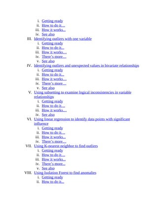
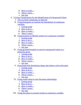

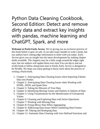


![pd.set_option('display.width', 85)
pd.set_option('display.max_columns', 8)
1. Read the data file, set new names for the headings, and parse the date
column.
Pass an argument of 1 to the skiprows parameter to skip the first row, pass
a list of columns to parse_dates to create a pandas datetime column from
those columns, and set low_memory to False to reduce the usage of memory
during the import process:
landtemps = pd.read_csv('data/landtempssample.csv',
... names=['stationid','year','month','avgtemp','latitude',
... 'longitude','elevation','station','countryid','country
'],
... skiprows=1,
... parse_dates=[['month','year']],
... low_memory=False)
>>> type(landtemps)
<class 'pandas.core.frame.DataFrame'>
Note
We have to use skiprows because we are passing a list of column
names to read_csv . If we use the column names in the CSV file
we do not need to specify values for either names or skiprows .
1. Get a quick glimpse of the data.
View the first few rows. Show the data type for all columns, as well as
the number of rows and columns:
>>> landtemps.head(7)
month_year stationid ... countryid
0 2000-04-01 USS0010K01S ... US
1 1940-05-01 CI000085406 ... CI
2 2013-12-01 USC00036376 ... US
3 1963-02-01 ASN00024002 ... AS
4 2001-11-01 ASN00028007 ... AS
5 1991-04-01 USW00024151 ... US
6 1993-12-01 RSM00022641 ... RS
country](https://image.slidesharecdn.com/28069340-250513003758-0935e9b1/85/Python-Data-Cleaning-Cookbook-Second-Edition-Michael-Walker-19-320.jpg)
![0 United States
1 Chile
2 United States
3 Australia
4 Australia
5 United States
6 Russia
[7 rows x 9 columns]
>>> landtemps.dtypes
month_year datetime64[ns]
stationid object
avgtemp float64
latitude float64
longitude float64
elevation float64
station object
countryid object
country object
dtype: object
>>> landtemps.shape
(100000, 9)
1. Give the date column a better name and view the summary statistics for
average monthly temperature:
>>> landtemps.rename(columns={'month_year':'measuredate'}, inpla
ce=True)
>>> landtemps.dtypes
measuredate datetime64[ns]
stationid object
avgtemp float64
latitude float64
longitude float64
elevation float64
station object
countryid object
country object
dtype: object
>>> landtemps.avgtemp.describe()
count 85,554.00
mean 10.92](https://image.slidesharecdn.com/28069340-250513003758-0935e9b1/85/Python-Data-Cleaning-Cookbook-Second-Edition-Michael-Walker-20-320.jpg)
![std 11.52
min -70.70
25% 3.46
50% 12.22
75% 19.57
max 39.95
Name: avgtemp, dtype: float64
1. Look for missing values for each column.
Use isnull , which returns True for each value that is missing for each
column, and False when not missing. Chain this with sum to count the
missings for each column. (When working with Boolean values, sum treats
True as 1 and False as 0 . I will discuss method chaining in the There’s
more... section of this recipe):
>>> landtemps.isnull().sum()
measuredate 0
stationid 0
avgtemp 14446
latitude 0
longitude 0
elevation 0
station 0
countryid 0
country 5
dtype: int64
1. Remove rows with missing data for avgtemp .
Use the subset parameter to tell dropna to drop rows when avgtemp is
missing. Set inplace to True . Leaving inplace at its default value of
False would display the DataFrame, but the changes we have made would
not be retained. Use the shape attribute of the DataFrame to get the number
of rows and columns:
>>> landtemps.dropna(subset=['avgtemp'], inplace=True)
>>> landtemps.shape
(85554, 9)
That’s it! Importing CSV files into pandas is as simple as that.](https://image.slidesharecdn.com/28069340-250513003758-0935e9b1/85/Python-Data-Cleaning-Cookbook-Second-Edition-Michael-Walker-21-320.jpg)
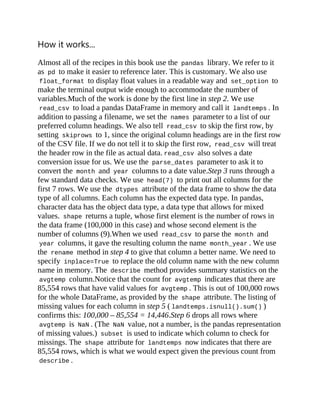
![There’s more...
If the file you are reading uses a delimiter other than a comma, such as a tab,
this can be specified in the sep parameter of read_csv . When creating the
pandas DataFrame, an index was also created. The numbers to the far left of
the output when head and sample were run are index values. Any number
of rows can be specified for head or sample . The default value is 5 .Setting
low_memory to False causes read_csv to parse data in chunks. This is
easier on systems with lower memory when working with larger files.
However, the full DataFrame will still be loaded into memory once
read_csv completes successfully.The landtemps.isnull().sum()
statement is an example of chaining methods. First, isnull returns a
DataFrame of True and False values, resulting from testing whether each
column value is null . sum takes that DataFrame and sums the True values
for each column, interpreting the True values as 1 and the False values as
0 . We would have obtained the same result if we had used the following two
steps:
>>> checknull = landtemps.isnull()
>>> checknull.sum()
There is no hard and fast rule for when to chain methods and when not to do
so. I find it helpful to chain when I really think of something I am doing as
being a single step, but only two or more steps, mechanically speaking.
Chaining also has the side benefit of not creating extra objects that I might
not need.The dataset used in this recipe is just a sample from the full land
temperatures database with almost 17 million records. You can run the larger
file if your machine can handle it, with the following code:
>>> landtemps = pd.read_csv('data/landtemps.zip',
... compression='zip', names=['stationid','year',
... 'month','avgtemp','latitude','longitude',
... 'elevation','station','countryid','country'],
... skiprows=1,
... parse_dates=[['month','year']],
... low_memory=False)
read_csv can read a compressed ZIP file. We get it to do this by passing the
name of the ZIP file and the type of compression.](https://image.slidesharecdn.com/28069340-250513003758-0935e9b1/85/Python-Data-Cleaning-Cookbook-Second-Edition-Michael-Walker-23-320.jpg)
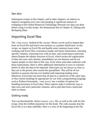
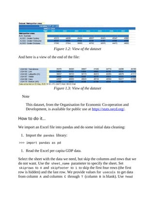
![to view the first few rows:
>>> percapitaGDP = pd.read_excel("data/GDPpercapita.xlsx",
... sheet_name="OECD.Stat export",
... skiprows=4,
... skipfooter=1,
... usecols="A,C:T")
>>> percapitaGDP.head()
Year 2001 2017 2018
0 Metropolitan areas NaN NaN NaN
1 AUS: Australia
2 AUS01: Greater Sydney 43313 50578 49860
3 AUS02: Greater Melbourne 40125 43025 42674
4 AUS03: Greater Brisbane 37580 46876 46640
[5 rows x 19 columns]
1. Use the info method of the data frame to view data types and the
non-null count:
>>> percapitaGDP.info()
<class 'pandas.core.frame.DataFrame'>
RangeIndex: 702 entries, 0 to 701
Data columns (total 19 columns):
# Column Non-Null Count Dtype
--- ------ -------------- -----
0 Year 702 non-null object
1 2001 701 non-null object
2 2002 701 non-null object
3 2003 701 non-null object
4 2004 701 non-null object
5 2005 701 non-null object
6 2006 701 non-null object
7 2007 701 non-null object
8 2008 701 non-null object
9 2009 701 non-null object
10 2010 701 non-null object
11 2011 701 non-null object
12 2012 701 non-null object
13 2013 701 non-null object
14 2014 701 non-null object
15 2015 701 non-null object
16 2016 701 non-null object
17 2017 701 non-null object
18 2018 701 non-null object
dtypes: object(19)](https://image.slidesharecdn.com/28069340-250513003758-0935e9b1/85/Python-Data-Cleaning-Cookbook-Second-Edition-Michael-Walker-26-320.jpg)
![memory usage: 104.3+ KB
1. Rename the Year column to metro and remove the leading spaces.
Give an appropriate name to the metropolitan area column. There are extra
spaces before the metro values in some cases, and extra spaces after the metro
values in others. We can test for leading spaces with startswith(‘ ‘) and then
use any to establish whether there are one or more occasions when the first
character is blank. We can use endswith(‘ ‘) to examine trailing spaces. We
use strip to remove both leading and trailing spaces. When we test for trailing
spaces again we see that there are none:
>>> percapitaGDP.rename(columns={'Year':'metro'}, inplace=True)
>>> percapitaGDP.metro.str.startswith(' ').any()
True
>>> percapitaGDP.metro.str.endswith(' ').any()
True
>>> percapitaGDP.metro = percapitaGDP.metro.str.strip()
percapitaGDP.metro.str.endswith(' ').any()
False
1. Convert the data columns to numeric.
Iterate over all of the GDP year columns (2001-2018) and convert the data
type from object to float . Coerce the conversion even when there is
character data – the .. in this example. We want character values in those
columns to become missing, which is what happens. Rename the year
columns to better reflect the data in those columns:
>>> for col in percapitaGDP.columns[1:]:
... percapitaGDP[col] = pd.to_numeric(percapitaGDP[col],
... errors='coerce')
... percapitaGDP.rename(columns={col:'pcGDP'+col},
... inplace=True)
...
metro pcGDP2001 ...
0 Metropolitan areas NaN ...
1 AUS: Australia NaN ...](https://image.slidesharecdn.com/28069340-250513003758-0935e9b1/85/Python-Data-Cleaning-Cookbook-Second-Edition-Michael-Walker-27-320.jpg)
![2 AUS01:Greater Sydney 43313 ...
3 AUS02: Greater Melbourne 40125 ...
4 AUS03: Greater Brisbane 37580 ...
pcGDP2017 pcGDP2018
0 NaN NaN
1 NaN NaN
2 50578 49860
3 43025 42674
4 46876 46640
[5 rows x 19 columns]
>>> percapitaGDP.dtypes
metro object
pcGDP2001 float64
pcGDP2002 float64
abbreviated to save space
pcGDP2017 float64
pcGDP2018 float64
dtype: object
1. Use the describe method to generate summary statistics for all
numeric data in the data frame:
>>> percapitaGDP.describe()
pcGDP2001 pcGDP2002 pcGDP2017 pcGDP2018
count 424 440 445 441
mean 41264 41015 47489 48033
std 11878 12537 15464 15720
min 10988 11435 2745 2832
25% 33139 32636 37316 37908
50% 39544 39684 45385 46057
75% 47972 48611 56023 56638
max 91488 93566 122242 127468
[8 rows x 18 columns]
1. Remove rows where all of the per capita GDP values are missing.
Use the subset parameter of dropna to inspect all columns, starting with
the second column (it is zero-based) through the last column. Use how to
specify that we want to drop rows only if all of the columns specified in
subset are missing. Use shape to show the number of rows and columns in
the resulting DataFrame:
>>> percapitaGDP.dropna(subset=percapitaGDP.columns[1:], how="al
l", inplace=True)](https://image.slidesharecdn.com/28069340-250513003758-0935e9b1/85/Python-Data-Cleaning-Cookbook-Second-Edition-Michael-Walker-28-320.jpg)
![>>> percapitaGDP.describe()
pcGDP2001 pcGDP2002 pcGDP2017 pcGDP2018
count 424 440 445 441
mean 41264 41015 47489 48033
std 11878 12537 15464 15720
min 10988 11435 2745 2832
25% 33139 32636 37316 37908
50% 39544 39684 45385 46057
75% 47972 48611 56023 56638
max 91488 93566 122242 127468
[8 rows x 18 columns]
>>> percapitaGDP.head()
metro pcGDP2001 pcGDP2002
2 AUS01: Greater Sydney 43313 44008
3 AUS02: Greater Melbourne 40125 40894
4 AUS03:Greater Brisbane 37580 37564
5 AUS04: Greater Perth 45713 47371
6 AUS05: Greater Adelaide 36505 37194
... pcGDP2016 pcGDP2017 pcGDP2018
2 ... 50519 50578 49860
3 ... 42671 43025 42674
4 ... 45723 46876 46640
5 ... 66032 66424 70390
6 ... 39737 40115 39924
[5 rows x 19 columns]
>>> percapitaGDP.shape
(480, 19)
1. Set the index for the DataFrame using the metropolitan area column.
Confirm that there are 480 valid values for metro and that there are 480
unique values, before setting the index:
>>> percapitaGDP.metro.count()
480
>>> percapitaGDP.metro.nunique()
480
>>> percapitaGDP.set_index('metro', inplace=True)
>>> percapitaGDP.head()
pcGDP2001 ... pcGDP2018
metro ...](https://image.slidesharecdn.com/28069340-250513003758-0935e9b1/85/Python-Data-Cleaning-Cookbook-Second-Edition-Michael-Walker-29-320.jpg)
![AUS01: Greater Sydney 43313 ... 49860
AUS02: Greater Melbourne 40125 ... 42674
AUS03: Greater Brisbane 37580 ... 46640
AUS04: Greater Perth 45713 ... 70390
AUS05: Greater Adelaide 36505 ... 39924
[5 rows x 18 columns]
>>> percapitaGDP.loc['AUS02: Greater Melbourne']
pcGDP2001 40125
pcGDP2002 40894
...
pcGDP2017 43025
pcGDP2018 42674
Name: AUS02: Greater Melbourne, dtype: float64
We have now imported the Excel data into a pandas data frame and cleaned
up some of the messiness in the spreadsheet.
How it works…
We mostly manage to get the data we want in step 2 by skipping rows and
columns we do not want, but there are still a number of issues: read_excel
interprets all of the GDP data as character data, many rows are loaded with
no useful data, and the column names do not represent the data well. In
addition, the metropolitan area column might be useful as an index, but there
are leading and trailing blanks and there may be missing or duplicated
values. read_excel interprets Year as the column name for the metropolitan
area data because it looks for a header above the data for that Excel column
and finds Year there. We rename that column metro in step 4. We also use
strip to fix the problem with leading and trailing blanks. If there had only
been leading blanks, we could have used lstrip , or rstrip if there had
only been trailing blanks. It is a good idea to assume that there might be
leading or trailing blanks in any character data and clean that data shortly
after the initial import.The spreadsheet authors used .. to represent missing
data. Since this is actually valid character data, those columns get the object
data type (that is how pandas treats columns with character or mixed data).
We coerce a conversion to numeric in step 5. This also results in the original
values of .. being replaced with NaN (not a number), pandas missing values
for numbers. This is what we want.We can fix all of the per capita GDP
columns with just a few lines because pandas makes it easy to iterate over the](https://image.slidesharecdn.com/28069340-250513003758-0935e9b1/85/Python-Data-Cleaning-Cookbook-Second-Edition-Michael-Walker-30-320.jpg)
![columns of a DataFrame. By specifying [1:] , we iterate from the second
column to the last column. We can then change those columns to numeric
and rename them to something more appropriate.There are several reasons
why it is a good idea to clean up the column headings for the annual GDP
columns: it helps us to remember what the data actually is; if we merge it
with other data by metropolitan area, we will not have to worry about
conflicting variable names; and we can use attribute access to work with
pandas series based on those columns, which I will discuss in more detail in
the There’s more… section of this recipe. describe in step 6 shows us that
fewer than 500 rows have valid data for per capita GDP. When we drop all
rows that have missing values for all per capita GDP columns in step 7, we
end up with 480 rows in the DataFrame.
There’s more…
Once we have a pandas DataFrame, we have the ability to treat columns as
more than just columns. We can use attribute access (such as
percapitaGPA.metro ) or bracket notation ( percapitaGPA[‘metro’] ) to get
the functionality of a pandas data series. Either method makes it possible to
use data series string inspecting methods such as str.startswith , and
counting methods such as nunique . Note that the original column names of
20## did not allow for attribute access because they started with a number,
so percapitaGDP.pcGDP2001.count() works, but
percapitaGDP.2001.count() returns a syntax error because 2001 is not a
valid Python identifier (since it starts with a number).pandas is rich with
features for string manipulation and for data series operations. We will try
many of them out in subsequent recipes. This recipe showed those I find most
useful when importing Excel data.
See also
There are good reasons to consider reshaping this data. Instead of 18 columns
of GDP per capita data for each metropolitan area, we should have 18 rows of
data for each metropolitan area, with columns for year and GDP per capita.
Recipes for reshaping data can be found in Chapter 9, Tidying and Reshaping
Data.](https://image.slidesharecdn.com/28069340-250513003758-0935e9b1/85/Python-Data-Cleaning-Cookbook-Second-Edition-Michael-Walker-31-320.jpg)
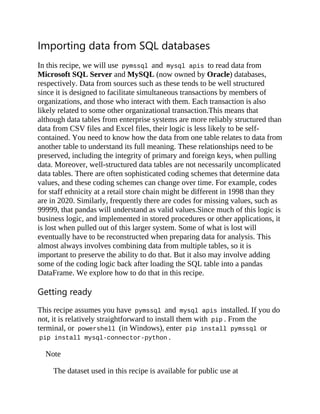
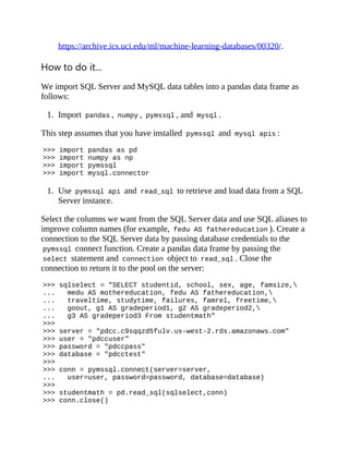
![1. Check the data types and the first few rows:
>>> studentmath.dtypes
studentid object
school object
sex object
age int64
famsize object
mothereducation int64
fathereducation int64
traveltime int64
studytime int64
failures int64
famrel int64
freetime int64
goout int64
gradeperiod1 int64
gradeperiod2 int64
gradeperiod3 int64
dtype: object
>>> studentmath.head()
studentid school ... gradeperiod2 gradeperiod3
0 001 GP ... 6 6
1 002 GP ... 5 6
2 003 GP ... 8 10
3 004 GP ... 14 15
4 005 GP ... 10 10
[5 rows x 16 columns]
1. (Alternative) Use the mysql connector and read_sql to get data from
MySQL.
Create a connection to the mysql data and pass that connection to read_sql
to retrieve the data and load it into a pandas data frame. (The same data file
on student math scores was uploaded to SQL Server and MySQL, so we can
use the same SQL select statement we used in the previous step.):
>>> host = "pdccmysql.c9sqqzd5fulv.us-west-2.rds.amazonaws.com"
>>> user = "pdccuser"
>>> password = "pdccpass"
>>> database = "pdccschema"
>>> connmysql = mysql.connector.connect(host=host,](https://image.slidesharecdn.com/28069340-250513003758-0935e9b1/85/Python-Data-Cleaning-Cookbook-Second-Edition-Michael-Walker-34-320.jpg)
![... database=database,user=user,password=password)
>>> studentmath = pd.read_sql(sqlselect,connmysql)
>>> connmysql.close()
1. Rearrange the columns, set an index, and check for missing values.
Move the grade data to the left of the DataFrame, just after studentid . Also
move the freetime column to the right after traveltime and studytime .
Confirm that each row has an ID and that the IDs are unique, and set
studentid as the index:
>>> newcolorder = ['studentid', 'gradeperiod1',
... 'gradeperiod2','gradeperiod3', 'school',
... 'sex', 'age', 'famsize','mothereducation',
... 'fathereducation', 'traveltime',
... 'studytime', 'freetime', 'failures',
... 'famrel','goout']
>>> studentmath = studentmath[newcolorder]
>>> studentmath.studentid.count()
395
>>> studentmath.studentid.nunique()
395
>>> studentmath.set_index('studentid', inplace=True)
1. Use the data frame’s count function to check for missing values:
>>> studentmath.count()
gradeperiod1 395
gradeperiod2 395
gradeperiod3 395
school 395
sex 395
age 395
famsize 395
mothereducation 395
fathereducation 395
traveltime 395
studytime 395
freetime 395
failures 395
famrel 395](https://image.slidesharecdn.com/28069340-250513003758-0935e9b1/85/Python-Data-Cleaning-Cookbook-Second-Edition-Michael-Walker-35-320.jpg)
![goout 395
dtype: int64
1. Replace coded data values with more informative values.
Create a dictionary with the replacement values for the columns, and then use
replace to set those values:
>>> setvalues=
... {"famrel":{1:"1:very bad",2:"2:bad",
... 3:"3:neutral",4:"4:good",5:"5:excellent"},
... "freetime":{1:"1:very low",2:"2:low",
... 3:"3:neutral",4:"4:high",5:"5:very high"},
... "goout":{1:"1:very low",2:"2:low",3:"3:neutral",
... 4:"4:high",5:"5:very high"},
... "mothereducation":{0:np.nan,1:"1:k-4",2:"2:5-9",
... 3:"3:secondary ed",4:"4:higher ed"},
... "fathereducation":{0:np.nan,1:"1:k-4",2:"2:5-9",
... 3:"3:secondary ed",4:"4:higher ed"}}
>>> studentmath.replace(setvalues, inplace=True)
1. Change the type for columns with the changed data to category .
Check any changes in memory usage:
>>> setvalueskeys = [k for k in setvalues]
>>> studentmath[setvalueskeys].memory_usage(index=False)
famrel 3160
freetime 3160
goout 3160
mothereducation 3160
fathereducation 3160
dtype: int64
>>> for col in studentmath[setvalueskeys].columns:
... studentmath[col] = studentmath[col].
... astype('category')
...
>>> studentmath[setvalueskeys].memory_usage(index=False)
famrel 607
freetime 607
goout 607
mothereducation 599](https://image.slidesharecdn.com/28069340-250513003758-0935e9b1/85/Python-Data-Cleaning-Cookbook-Second-Edition-Michael-Walker-36-320.jpg)
![fathereducation 599
dtype: int64
1. Calculate percentages for values in the famrel column.
Run value_counts and set normalize to True to generate percentages:
>>> studentmath['famrel'].value_counts(sort=False, normalize=Tru
e)
1:very bad 0.02
2:bad 0.05
3:neutral 0.17
4:good 0.49
5:excellent 0.27
Name: famrel, dtype: float64
1. Use apply to calculate percentages for multiple columns:
>>> studentmath[['freetime','goout']].
... apply(pd.Series.value_counts, sort=False,
... normalize=True)
freetime goout
1:very low 0.05 0.06
2:low 0.16 0.26
3:neutral 0.40 0.33
4:high 0.29 0.22
5:very high 0.10 0.13
>>> studentmath[['mothereducation','fathereducation']].
... apply(pd.Series.value_counts, sort=False,
... normalize=True)
mothereducation fathereducation
1:k-4 0.15 0.21
2:5-9 0.26 0.29
3:secondary ed 0.25 0.25
4:higher ed 0.33 0.24
The preceding steps retrieved a data table from a SQL database, loaded that
data into pandas, and did some initial data checking and cleaning.
How it works…](https://image.slidesharecdn.com/28069340-250513003758-0935e9b1/85/Python-Data-Cleaning-Cookbook-Second-Edition-Michael-Walker-37-320.jpg)
![Since data from enterprise systems is typically better structured than CSV or
Excel files, we do not need to do things such as skip rows or deal with
different logical data types in a column. But some massaging is still usually
required before we can begin exploratory analysis. There are often more
columns than we need, and some column names are not intuitive or not
ordered in the best way for analysis. The meaningfulness of many data values
is not stored in the data table, to avoid entry errors and save on storage space.
For example, 3 is stored for mother’s education rather than
secondary education . It is a good idea to reconstruct that coding as early in
the cleaning process as possible.To pull data from a SQL database server, we
need a connection object to authenticate us on the server, and a SQL select
string. These can be passed to read_sql to retrieve the data and load it into a
pandas DataFrame. I usually use the SQL SELECT statement to do a bit of
cleanup of column names at this point. I sometimes also reorder columns, but
I do that later in this recipe.We set the index in step 5, first confirming that
every row has a value for studentid and that it is unique. This is often more
important when working with enterprise data because we will almost always
need to merge the retrieved data with other data files on the system. Although
an index is not required for this merging, the discipline of setting one
prepares us for the tricky business of merging data down the road. It will also
likely improve the speed of the merge.We use the DataFrame’s count
function to check for missing values and there are no missing values – non-
missing values is 395 (the number of rows) for every column. This is almost
too good to be true. There may be values that are logically missing; that is,
valid numbers that nonetheless connote missing values, such as -1, 0, 9, or
99. We address this possibility in the next step.Step 7 demonstrates a useful
technique for replacing data values for multiple columns. We create a
dictionary to map original values to new values for each column, and then
run it using replace . To reduce the amount of storage space taken up by the
new verbose values, we convert the data type of those columns to category .
We do this by generating a list of the keys of our setvalues dictionary –
setvalueskeys = [k for k in setvalues] generates [ famrel ,
freetime , goout , mothereducation , and fathereducation ]. We then
iterate over those five columns and use the astype method to change the
data type to category . Notice that the memory usage for those columns is
reduced substantially.Finally, we check the assignment of new values by
using value_counts to view relative frequencies. We use apply because](https://image.slidesharecdn.com/28069340-250513003758-0935e9b1/85/Python-Data-Cleaning-Cookbook-Second-Edition-Michael-Walker-38-320.jpg)
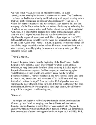
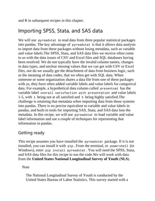
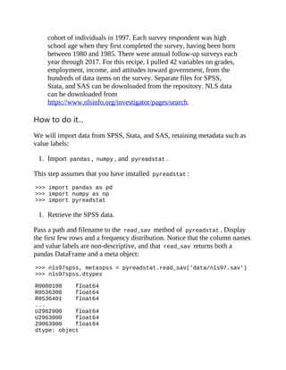
![>>> nls97spss.head()
R0000100 R0536300 ... U2963000 Z9063900
0 1 2 ... nan 52
1 2 1 ... 6 0
2 3 2 ... 6 0
3 4 2 ... 6 4
4 5 1 ... 5 12
[5 rows x 42 columns]
>>> nls97spss['R0536300'].value_counts(normalize=True)
1.00 0.51
2.00 0.49
Name: R0536300, dtype: float64
1. Grab the metadata to improve column labels and value labels.
The metaspss object created when we called read_sav has the column
labels and the value labels from the SPSS file. Use the
variable_value_labels dictionary to map values to value labels for one
column ( R0536300 ). (This does not change the data. It only improves our
display when we run value_counts .) Use the set_value_labels method to
actually apply the value labels to the DataFrame:
>>> metaspss.variable_value_labels['R0536300']
{0.0: 'No Information', 1.0: 'Male', 2.0: 'Female'}
>>> nls97spss['R0536300'].
... map(metaspss.variable_value_labels['R0536300']).
... value_counts(normalize=True)
Male 0.51
Female 0.49
Name: R0536300, dtype: float64
>>> nls97spss = pyreadstat.set_value_labels(nls97spss, metaspss,
formats_as_category=True)
1. Use column labels in the metadata to rename the columns.
To use the column labels from metaspss in our DataFrame, we can
simply assign the column labels in metaspss to our DataFrame’s
column names. Clean up the column names a bit by changing them to
lowercase, changing spaces to underscores, and removing all remaining](https://image.slidesharecdn.com/28069340-250513003758-0935e9b1/85/Python-Data-Cleaning-Cookbook-Second-Edition-Michael-Walker-42-320.jpg)
![non-alphanumeric characters:
>>> nls97spss.columns = metaspss.column_labels
>>> nls97spss['KEY!SEX (SYMBOL) 1997'].value_counts(normalize=Tr
ue)
Male 0.51
Female 0.49
Name: KEY!SEX (SYMBOL) 1997, dtype: float64
>>> nls97spss.dtypes
PUBID - YTH ID CODE 1997 float64
KEY!SEX (SYMBOL) 1997 category
KEY!BDATE M/Y (SYMBOL) 1997 float64
KEY!BDATE M/Y (SYMBOL) 1997 float64
CV_SAMPLE_TYPE 1997 category
KEY!RACE_ETHNICITY (SYMBOL) 1997 category
HRS/WK R WATCHES TELEVISION 2017 category
HRS/NIGHT R SLEEPS 2017 float64
CVC_WKSWK_YR_ALL L99 float64
dtype: object
>>> nls97spss.columns = nls97spss.columns.
... str.lower().
... str.replace(' ','_').
... str.replace('[^a-z0-9_]', '')
>>> nls97spss.set_index('pubid__yth_id_code_1997', inplace=True)
1. Simplify the process by applying the value labels from the beginning.
The data values can actually be applied in the initial call to read_sav by
setting apply_value_formats to True . This eliminates the need to call the
set_value_labels function later:
>>> nls97spss, metaspss = pyreadstat.read_sav('data/nls97.sav',
apply_value_formats=True, formats_as_category=True)
>>> nls97spss.columns = metaspss.column_labels
>>> nls97spss.columns = nls97spss.columns.
... str.lower().
... str.replace(' ','_').
... str.replace('[^a-z0-9_]', '')
1. Show the columns and a few rows:
>>> nls97spss.dtypes](https://image.slidesharecdn.com/28069340-250513003758-0935e9b1/85/Python-Data-Cleaning-Cookbook-Second-Edition-Michael-Walker-43-320.jpg)
![pubid__yth_id_code_1997 float64
keysex_symbol_1997 category
keybdate_my_symbol_1997 float64
keybdate_my_symbol_1997 float64
hrsnight_r_sleeps_2017 float64
cvc_wkswk_yr_all_l99 float64
dtype: object
>>> nls97spss.head()
pubid__yth_id_code_1997 keysex_symbol_1997 ...
0 1 Female ...
1 2 Male ...
2 3 Female ...
3 4 Female ...
4 5 Male ...
hrsnight_r_sleeps_2017 cvc_wkswk_yr_all_l99
0 nan 52
1 6 0
2 6 0
3 6 4
4 5 12
[5 rows x 42 columns]
1. Run frequencies on one of the columns and set the index:
>>> nls97spss.govt_responsibility__provide_jobs_2006.
... value_counts(sort=False)
Definitely should be 454
Definitely should not be 300
Probably should be 617
Probably should not be 462
Name: govt_responsibility__provide_jobs_2006, dtype: int64
>>> nls97spss.set_index('pubid__yth_id_code_1997', inplace=True)
1. Import the Stata data, apply value labels, and improve the column
headings.
Use the same methods for the Stata data that we use for the SPSS data:
>>> nls97stata, metastata = pyreadstat.read_dta('data/nls97.dta'
, apply_value_formats=True, formats_as_category=True)
>>> nls97stata.columns = metastata.column_labels](https://image.slidesharecdn.com/28069340-250513003758-0935e9b1/85/Python-Data-Cleaning-Cookbook-Second-Edition-Michael-Walker-44-320.jpg)
![>>> nls97stata.columns = nls97stata.columns.
... str.lower().
... str.replace(' ','_').
... str.replace('[^a-z0-9_]', '')
>>> nls97stata.dtypes
pubid__yth_id_code_1997 float64
keysex_symbol_1997 category
keybdate_my_symbol_1997 float64
keybdate_my_symbol_1997 float64
hrsnight_r_sleeps_2017 float64
cvc_wkswk_yr_all_l99 float64
dtype: object
1. View a few rows of the data and run a frequency :
>>> nls97stata.head()
pubid__yth_id_code_1997 keysex_symbol_1997 ...
0 1 Female ...
1 2 Male ...
2 3 Female ...
3 4 Female ...
4 5 Male ...
hrsnight_r_sleeps_2017 cvc_wkswk_yr_all_l99
0 -5 52
1 6 0
2 6 0
3 6 4
4 5 12
[5 rows x 42 columns]
>>> nls97stata.govt_responsibility__provide_jobs_2006.
... value_counts(sort=False)
-5.0 1425
-4.0 5665
-2.0 56
-1.0 5
Definitely should be 454
Definitely should not be 300
Probably should be 617
Probably should not be 462
Name: govt_responsibility__provide_jobs_2006, dtype: int64](https://image.slidesharecdn.com/28069340-250513003758-0935e9b1/85/Python-Data-Cleaning-Cookbook-Second-Edition-Michael-Walker-45-320.jpg)
![1. Fix the logical missing values that show up with the Stata data and set
an index:
>>> nls97stata.min()
pubid__yth_id_code_1997 1
keysex_symbol_1997 Female
keybdate_my_symbol_1997 1
keybdate_my_symbol_1997 1,980
cv_bio_child_hh_2017 -5
cv_bio_child_nr_2017 -5
hrsnight_r_sleeps_2017 -5
cvc_wkswk_yr_all_l99 -4
dtype: object
>>> nls97stata.replace(list(range(-9,0)), np.nan, inplace=True)
>>> nls97stata.min()
pubid__yth_id_code_1997 1
keysex_symbol_1997 Female
keybdate_my_symbol_1997 1
keybdate_my_symbol_1997 1,980
cv_bio_child_hh_2017 0
cv_bio_child_nr_2017 0
hrsnight_r_sleeps_2017 0
cvc_wkswk_yr_all_l99 0
dtype: object
>>> nls97stata.set_index('pubid__yth_id_code_1997', inplace=True)
1. Retrieve the SAS data, using the SAS catalog file for value labels:
The data values for SAS are stored in a catalog file. Setting the catalog file
path and filename retrieves the value labels and applies them:
>>> nls97sas, metasas = pyreadstat.read_sas7bdat('data/nls97.sas
7bdat', catalog_file='data/nlsformats3.sas7bcat', formats_as_cat
egory=True)
>>> nls97sas.columns = metasas.column_labels
>>>
>>> nls97sas.columns = nls97sas.columns.
... str.lower().
... str.replace(' ','_').
... str.replace('[^a-z0-9_]', '')
>>>
>>> nls97sas.head()](https://image.slidesharecdn.com/28069340-250513003758-0935e9b1/85/Python-Data-Cleaning-Cookbook-Second-Edition-Michael-Walker-46-320.jpg)
![pubid__yth_id_code_1997 keysex_symbol_1997 ...
0 1 Female ...
1 2 Male ...
2 3 Female ...
3 4 Female ...
4 5 Male ...
hrsnight_r_sleeps_2017 cvc_wkswk_yr_all_l99
0 nan 52
1 6 0
2 6 0
3 6 4
4 5 12
[5 rows x 42 columns]
>>> nls97sas.keysex_symbol_1997.value_counts()
Male 4599
Female 4385
Name: keysex_symbol_1997, dtype: int64
>>> nls97sas.set_index('pubid__yth_id_code_1997', inplace=True)
This demonstrates how to import SPSS, SAS, and Stata data without losing
important metadata.
How it works...
The read_sav , read_dta , and read_sas7bdat methods of Pyreadstat ,
for SPSS, Stata, and SAS data files, respectively, work in a similar manner.
Value labels can be applied when reading in the data by setting
apply_value_formats to True for SPSS and Stata files (steps 5 and 8), or
by providing a catalog file path and filename for SAS (step 11). We can set
formats_as_category to True to change the data type to category for
those columns where the data values will change. The meta object has the
column names and the column labels from the statistical package, so
metadata column labels can be assigned to pandas data frame column names
at any point ( nls97spss.columns = metaspss.column_labels ). We can
even revert to the original column headings after assigning meta column
labels to them by setting pandas column names to the metadata column
names ( nls97spss.columns = metaspss.column_names ).In step 3, we read](https://image.slidesharecdn.com/28069340-250513003758-0935e9b1/85/Python-Data-Cleaning-Cookbook-Second-Edition-Michael-Walker-47-320.jpg)
![the SPSS data without applying value labels. We looked at the dictionary for
one variable ( metaspss.variable_value_labels['R0536300'] ), but we
could have viewed it for all variables ( metaspss.variable_value_labels ).
When we are satisfied that the labels make sense, we can set them by calling
the set_value_labels function. This is a good approach when you do not
know the data well and want to inspect the labels before applying them.The
column labels from the meta object are often a better choice than the original
column headings. Column headings can be quite cryptic, particularly when
the SPSS, Stata, or SAS file is based on a large survey, as in this example.
But the labels are not usually ideal for column headings either. They
sometimes have spaces, capitalization that is not helpful, and non-
alphanumeric characters. We chain some string operations to switch to
lowercase, replace spaces with underscores, and remove non-alphanumeric
characters.Handling missing values is not always straightforward with these
data files, since there are often many reasons why data is missing. If the file
is from a survey, the missing value may be because of a survey skip pattern,
or a respondent failed to respond, or the response was invalid, and so on. The
National Longitudinal Survey has 9 possible values for missing, from -1 to
-9. The SPSS import automatically set those values to NaN , while the Stata
import retained the original values. (We could have gotten the SPSS import
to retain those values by setting user_missing to True .) For the Stata data,
we need to tell it to replace all values from -1 to -9 with NaN . We do this by
using the DataFrame’s replace function and passing it a list of integers
from -9 to -1 ( list(range(-9,0)) ).
There’s more…
You may have noticed similarities between this recipe and the previous one
in terms of how value labels are set. The set_value_labels function is like
the DataFrame replace operation we used to set value labels in that recipe.
We passed a dictionary to replace that mapped columns to value labels.
The set_value_labels function in this recipe essentially does the same
thing, using the variable_value_labels property of the meta object as the
dictionary.Data from statistical packages is often not as well structured as
SQL databases tend to be in one significant way. Since they are designed to
facilitate analysis, they often violate database normalization rules. There is
often an implied relational structure that might have to be unflattened at some](https://image.slidesharecdn.com/28069340-250513003758-0935e9b1/85/Python-Data-Cleaning-Cookbook-Second-Edition-Michael-Walker-48-320.jpg)
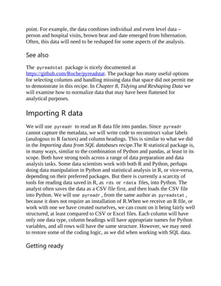
![This recipe assumes you have installed the pyreadr package. If it is not
installed, you can install it with pip . From the terminal, or powershell (in
Windows), enter pip install pyreadr .We will again work with the
National Longitudinal Survey in this recipe. You will need to download the
rds file used in this recipe from the GitHub repository in order to run the
code.
How to do it…
We will import data from R without losing important metadata:
1. Load pandas , numpy , pprint , and the pyreadr package:
>>> import pandas as pd
>>> import numpy as np
>>> import pyreadr
>>> import pprint
1. Get the R data.
Pass the path and filename to the read_r method to retrieve the R data and
load it into memory as a pandas DataFrame. read_r can return one or more
objects. When reading an rds file (as opposed to an rdata file), it will
return one object, having the key None . We indicate None to get the pandas
DataFrame:
>>> nls97r = pyreadr.read_r('data/nls97.rds')[None]
>>> nls97r.dtypes
R0000100 int32
R0536300 int32
...
U2962800 int32
U2962900 int32
U2963000 int32
Z9063900 int32
dtype: object
>>> nls97r.head(10)
R0000100 R0536300 ... U2963000 Z9063900
0 1 2 ... -5 52](https://image.slidesharecdn.com/28069340-250513003758-0935e9b1/85/Python-Data-Cleaning-Cookbook-Second-Edition-Michael-Walker-50-320.jpg)
![1 2 1 ... 6 0
2 3 2 ... 6 0
3 4 2 ... 6 4
4 5 1 ... 5 12
5 6 2 ... 6 6
6 7 1 ... -5 0
7 8 2 ... -5 39
8 9 1 ... 4 0
9 10 1 ... 6 0
[10 rows x 42 columns]
1. Set up dictionaries for value labels and column headings.
Load a dictionary that maps columns to the value labels and create a list of
preferred column names as follows:
>>> with open('data/nlscodes.txt', 'r') as reader:
... setvalues = eval(reader.read())
...
>>> pprint.pprint(setvalues)
{'R0536300': {0.0: 'No Information', 1.0: 'Male', 2.0: 'Female'}
,
'R1235800': {0.0: 'Oversample', 1.0: 'Cross-sectional'},
'S8646900': {1.0: '1. Definitely',
2.0: '2. Probably ',
3.0: '3. Probably not',
4.0: '4. Definitely not'}}
>>> newcols = ['personid','gender','birthmonth',
... 'birthyear','sampletype','category',
... 'satverbal','satmath','gpaoverall',
... 'gpaeng','gpamath','gpascience','govjobs',
... 'govprices','govhealth','goveld','govind',
... 'govunemp','govinc','govcollege',
... 'govhousing','govenvironment','bacredits',
... 'coltype1','coltype2','coltype3','coltype4',
... 'coltype5','coltype6','highestgrade',
... 'maritalstatus','childnumhome','childnumaway',
... 'degreecol1','degreecol2','degreecol3',
... 'degreecol4','wageincome','weeklyhrscomputer',
... 'weeklyhrstv','nightlyhrssleep',
... 'weeksworkedlastyear']
1. Set value labels and missing values, and change selected columns to
category data type.](https://image.slidesharecdn.com/28069340-250513003758-0935e9b1/85/Python-Data-Cleaning-Cookbook-Second-Edition-Michael-Walker-51-320.jpg)
![Use the setvalues dictionary to replace existing values with value labels.
Replace all values from -9 to -1 with NaN :
>>> nls97r.replace(setvalues, inplace=True)
>>> nls97r.head()
R0000100 R0536300 ... U2963000 Z9063900
0 1 Female ... -5 52
1 2 Male ... 6 0
2 3 Female ... 6 0
3 4 Female ... 6 4
4 5 Male ... 5 12
[5 rows x 42 columns]
>>> nls97r.replace(list(range(-9,0)), np.nan, inplace=True)
>>> for col in nls97r[[k for k in setvalues]].columns:
... nls97r[col] = nls97r[col].astype('category')
...
>>> nls97r.dtypes
R0000100 int64
R0536300 category
R0536401 int64
R0536402 int64
R1235800 category
...
U2857300 category
U2962800 category
U2962900 category
U2963000 float64
Z9063900 float64
Length: 42, dtype: object
1. Set meaningful column headings:
>>> nls97r.columns = newcols
>>> nls97r.dtypes
personid int64
gender category
birthmonth int64
birthyear int64
sampletype category
...
wageincome category
weeklyhrscomputer category
weeklyhrstv category](https://image.slidesharecdn.com/28069340-250513003758-0935e9b1/85/Python-Data-Cleaning-Cookbook-Second-Edition-Michael-Walker-52-320.jpg)
![nightlyhrssleep float64
weeksworkedlastyear float64
Length: 42, dtype: object
This shows how R data files can be imported into pandas and value labels
assigned.
How it works…
Reading R data into pandas with pyreadr is fairly straightforward. Passing a
filename to the read_r function is all that is required. Since read_r can
return multiple objects with one call, we need to specify which object. When
reading an rds file (as opposed to an rdata file), only one object is
returned. It has the key None .In step 3, we load a dictionary that maps our
variables to value labels, and a list for our preferred column headings. In step
4 we apply the value labels. We also change the data type to category for
the columns where we applied the values. We do this by generating a list of
the keys of our setvalues dictionary with [k for k in setvalues] and
then iterating over those columns.We change the column headings in step 5
to ones that are more intuitive. Note that the order matters here. We need to
set the value labels before changing the column names, since the setvalues
dictionary is based on the original column headings.The main advantage of
using pyreadr to read R files directly into pandas is that we do not have to
convert the R data into a CSV file first. Once we have written our Python
code to read the file, we can just rerun it whenever the R data changes. This is
particularly helpful when we do not have R on the machine where we are
working.
There’s more…
Pyreadr is able to return multiple data frames. This is useful when we save
several data objects in R as an rdata file. We can return all of them with one
call. Pprint is a handy tool for improving the display of Python dictionaries.
See also
Clear instructions and examples for pyreadr are available at](https://image.slidesharecdn.com/28069340-250513003758-0935e9b1/85/Python-Data-Cleaning-Cookbook-Second-Edition-Michael-Walker-53-320.jpg)
![https://github.com/ofajardo/pyreadr.Feather files, a relatively new format, can
be read by both R and Python. I discuss those files in the next recipe.We
could have used rpy2 instead of pyreadr to import R data. rpy2 requires
that R also be installed, but it is more powerful than pyreadr . It will read R
factors and automatically set them to pandas DataFrame values. See the
following code:
>>> import rpy2.robjects as robjects
>>> from rpy2.robjects import pandas2ri
>>> pandas2ri.activate()
>>> readRDS = robjects.r['readRDS']
>>> nls97withvalues = readRDS('data/nls97withvalues.rds')
>>> nls97withvalues
R0000100 R0536300 ... U2963000 Z9063900
1 1 Female ... -2147483648 52
2 2 Male ... 6 0
3 3 Female ... 6 0
4 4 Female ... 6 4
5 5 Male ... 5 12
... ... ... ... ... ...
8980 9018 Female ... 4 49
8981 9019 Male ... 6 0
8982 9020 Male ... -2147483648 15
8983 9021 Male ... 7 50
8984 9022 Female ... 7 20
[8984 rows x 42 columns]
This generates unusual -2147483648 values. This is what happened when
readRDS interpreted missing data in numeric columns. A global replace of
that number with NaN , after confirming that that is not a valid value, would
be a good next step.
Persisting tabular data
We persist data, copy it from memory to local or remote storage, for several
reasons: to be able to access the data without having to repeat the steps we
used to generate it; to share the data with others; or to make it available for
use with different software. In this recipe, we save data that we have loaded
into a pandas data frame as different file types (CSV, Excel, Pickle, and
Feather).Another important, but sometimes overlooked, reason to persist data](https://image.slidesharecdn.com/28069340-250513003758-0935e9b1/85/Python-Data-Cleaning-Cookbook-Second-Edition-Michael-Walker-54-320.jpg)