This document summarizes observations of molecular gas and star formation in the NGC 7000 molecular cloud and HII region. The key points are: 1. Five dense molecular clumps were identified in NGC 7000 based on NH3 emission, with sizes of 0.2-1 pc and masses of 9-452 solar masses. 2. The clumps have similar gas temperatures of 11-15K but different levels of star formation activity, from concentrations of T-Tauri stars to associations with H2O maser sources. 3. The star formation activities appear related to the geometry of the HII region, with the clump near the HII region boundary having the highest star formation efficiency of 36

1. PASJ: Publ. Astron. Soc. Japan , 1–??,
c 2011. Astronomical Society of Japan.
Propagation of Highly Efficient Star Formation in NGC 7000
Hideyuki Toujima,1 Takumi Nagayama,2 Toshihiro Omodaka,1, 3 Toshihiro Handa,4*
Yasuhiro Koyama,5 and Hideyuki Kobayashi2
1
Graduate School of Science and Engineering, Kagoshima University,
1-21-35 Korimoto, Kagoshima, Kagoshima 890-0065
2
Mizusawa VLBI Observatory, National Astronomical Observatory of Japan,
2-21-1 Osawa, Mitaka, Tokyo 181-8588
arXiv:1107.4177v1 [astro-ph.GA] 21 Jul 2011
3
Faculty of Science, Kagoshima University,
1-21-35 Korimoto, Kagoshima, Kagoshima 890-0065
4
Institute of Astronomy, The Universe of Tokyo,
2-21-1 Osawa, Mitaka, Tokyo 181-0015
5
Kashima Space Research Center, National Institute of Information and Communications Technology,
893-1 Hirai, Kashima, Ibaraki 314-8510
takumi.nagayama@nao.ac.jp
(Received 2009 October 6; accepted 2011 July 11)
Abstract
We surveyed the (1,1), (2,2), and (3,3) lines of NH3 and the H2 O maser toward the molecular cloud
′
L935 in the extended H II region NGC 7000 with an angular resolution of 1. 6 using the Kashima 34-m
telescope. We found five clumps in the NH3 emission with a size of 0.2–1 pc and mass of 9–452 M⊙ .
The molecular gas in these clumps has a similar gas kinetic temperature of 11–15 K and a line width of
1–2 km s−1 . However, they have different star formation activities such as the concentration of T-Tauri
type stars and the association of H2 O maser sources. We found that these star formation activities are
related to the geometry of the H II region. The clump associated with the T-Tauri type star cluster has a
high star formation efficiency of 36–62%. This clump is located near the boundary of the H II region and
molecular cloud. Therefore, we suggest that the star formation efficiency increases because of the triggered
star formation.
Key words: Star: formation - ISM: H II region - ISM: individual (SFR) - line (NH3 )
1. Introduction Figure 1 shows the optical image of NGC 7000 and L935.
Seven T-Tauri stars are clearly clustered at the boundary
The star formation efficiencies (SFEs) of molecular of the H II region (Herbig 1958). This suggests that the
clouds in the Milky Way Galaxy, are typically observed star formation is triggered by the interaction of the H II
to be 10%. The SFEs in nearby molecular clouds are ≃ region with the dense molecular gas. A number of studies
3–15% (Swift & Welch 2008; Evans et al. 2009). The ob- of star formation in a cloud associated with an H II re-
servations of giant molecular clouds in the inner Galaxy gion have been performed (Sugitani et al. 1989; Sugitani
indicate that the SFEs in these clouds are of the order of et al. 1991; Sugitani & Ogura 1994; Dobashi et al. 2001
a few percent (Myers et al. 1986). However, Lada (1992) Deharveng et al. 2003; Deharveng et al. 2005). For exam-
found that three of five massive cores, NGC 2024, NGC ple, in the nearby H II region, IC 5070, a molecular shell
2068, and NGC 2071 exhibit higher SFEs of ≃ 30–40%. with an expanding velocity of 5 km s−1 , is found in the
It remains unclear why these SFEs are high. Lada (1992) 12
CO (J=1-0) line (Bally & Scoville 1980). They suggest
suggested that the high gas densities and high gas mass that the T-Tauri type stars in IC 5070 are formed by the
may be required for the high SFE but there should be expanding shell.
additional conditions, because the other two cores exhibit Our aim is to investigate the relationship between dense
low SFEs of ≃ 7%. However, additional conditions for high molecular gas and star formation based on the SFE.
SFE are unknown, and more observational investigations NGC700 has the advantage of allowing us to estimate the
are required. ∗ SFE because T-Tauri type stars are associated with it and
NGC 7000 is an extended H II region in the Cygnus we can estimate the stellar mass accurately. Therefore,
X region. On its southeastern side is a molecular cloud we made the observations in the NH3 line to estimate the
L935. The 13 CO emission in this molecular cloud is the mass of dense molecular gas. We also surveyed an H2 O
brightest in the Cygnus X region (Dobashi et al. 1994). maser source that is associated with outflow from a young
∗ stellar object (YSO). We adopted the distance to NGC
Present address: Graduate School of Science and Engineering,
Kagoshima University, 1-21-35 Korimoto, Kagoshima, 7000 to be 600 pc (Laugalys & Straiˇys 2002).
z
Kagoshima 890-0065.

2. 2 H. Toujima et al. [Vol. ,
2. Observations The VLBI observations of the 616 → 523 transition of
the H2 O maser were made with the VERA of the National
2.1. NH3 Observations
Astronomical Observatory of Japan (NAOJ) on February
We observed NGC 7000 in the NH3 lines with the 15, 2008. The data were recorded using the VSOP termi-
Kashima 34-m telescope of the National institute of nal at a rate of 128 Mbit s−1 . The recorded signals were
Information and Communications Technology (NiCT) correlated using the Mitaka FX correlator. The spectral
from April 2007 to October 2008. We made simulta- resolution was set at 31.25 kHz, which corresponds to a
neous observations in three inversion transitions of the velocity resolution of 0.42 km s−1 . The system noise tem-
NH3 (J, K) = (1,1), (2,2), and (3,3) lines at 23.694495, perature is approximately 140 K. The phase calibrator was
23.722633, and 23.870129 GHz, respectively. At 23 GHz, BL Lac (ICRF J220243.2+421639). The phase-tracking
′
the telescope beam size was 1. 6 and the main beam ef- center of the array was set at α(J2000) = 20h 57m 56. 717,
s
◦ ′ ′′
ficiency (ηMB ) was 0.50. We used a K-band HEMT δ(J2000) = +43 53 39. 60. We calibrated the data in
amplifier whose system noise temperature was 150–250 the standard reduction procedure with the Astronomical
′
K. The relative pointing error was better than 0. 2; this Image Processing System (AIPS) of the National Radio
was checked by the observations of several H2 O maser Astronomy Observatory (NRAO). The resultant rms noise
sources at 22.235080 GHz. All spectra were obtained level and synthesized beam size are ≃ 1 Jy beam−1 and
with an 8192-channel FX-type spectrometer developed at ≃ 1.4 × 0.7 mas with a position angle of −46◦ .
Kagoshima University and NiCT. Its bandwidth and fre-
quency resolution are 256 MHz and 31.25 kHz, respec- 3. Results
tively. The corresponding velocity coverage and velocity
3.1. Distribution of NH3 Clumps
resolutions are 3200 km s−1 and 0.39 km s−1 at the NH3
frequencies, respectively. The total number of the ob- We observed 311 positions in the survey. NH3 (1,1)
served positions is 311 and the surveyed area is approxi- and (2,2) lines were detected with a signal-to-noise ratio
mately 38′ × 11′ or 6.6 pc × 1.9 pc. The NH3 profiles were greater than 3 at 138 and 32 positions, respectively. The
obtained at 1′ grid points of the equatorial coordinates. (3,3) line was not detected at any positions in the ob-
All data were obtained with the position switch between served area. We show the profiles towards emission peaks
the target and a reference position. The reference position in Figure 2.
is (α,δ)(J2000) = (20h58m 02. 1,+44◦04′ 24′′ ), where no NH3
s
Figure 3 shows the velocity integrated map of the main
emission was detected. We integrated at least 20 min at hyperfine component of the NH3 (1,1) line over vLSR = −3
each point. The rms noise level was typically 0.20 K in to 8 km s−1 . The NH3 (1,1) emission extends over 38′ ×
the unit of the main beam brightness temperature defined 11′ or 6.6 pc × 1.9 pc. The distribution is elongated in
∗ ∗
by TMB ≡ TA /ηMB , where TA is the antenna temperature the northeast-southwest direction.
calibrated by the chopper wheel method (Kutner & Ulich We define a clump as an isolated feature in the (1,1)
1981). integrated intensity distribution with intensities stronger
Data reduction was performed using the UltraSTAR than the 3σ noise level (> 0.6 K km s−1 ) both in the (1,1)
∼
package developed by the radio astronomy group at the and the (2,2) lines. Based on this definition, we identify
University of Tokyo (Nakajima et al. 2007). In this paper, two NH3 clumps; we call them clump-A at the northeast
the intensities are presented in the main beam tempera- and clump-B at the southwest. We found local peaks in
ture. these clumps. In clump-A, there are YSOs that may have
been formed near three local peaks (see subsection 4.1).
2.2. H2 O Maser Observations
In order to investigate the star formation of clump-A in
The single-dish observations of the 616 → 523 transi- detail, we define three subclumps as three local peaks in
tion of the H2 O maser at 22.235080 GHz were made at clump-A. We call them subclump-A1, subclump-A2, and
the positions of the NH3 emission peaks. The observa- subclump-A3 from the east to the west. The parameters
tions were made with the Kashima 34-m telescope and the of the clumps and subclumps are summarized in Table
VLBI Exploration of Radio Astrometry (VERA) Iriki 20- 1. As shown in Figure 3, the shape of these subclumps
m telescope. In the observations made with the Kashima appears to be an ellipse with the major axis along the
34-m telescope, the conversion factor from the antenna right ascension and the minor axis along the declination.
temperature to the flux density was 8 Jy K−1 for a point Therefore, we estimate the subclump sizes of the major
source. The rms noise level of the H2 O maser spectra was and minor axes using the FWHM of the Gaussian fitting
less than 1 Jy after integration of 10–30 min. The veloc- to the intensities along the right ascension and declination,
ity resolution of the spectrometer was 0.42 km s−1 at the respectively. Figure 4 shows the results of the Gaussian
H2 O maser frequency. In the observations made with the fitting. This size is used to estimate the mass of each
VERA Iriki 20-m telescope, the conversion factor from the subclump.
antenna temperature to the flux density was 20 Jy K−1 . Clump-A extends over 11′ × 10′ or 1.9 pc × 1.8 pc
The rms noise level of the H2 O maser spectra was less (Figure 3). The velocity channel maps from vLSR = 0 to
than 1 Jy after integration of 30 min. The velocity res- 8 km s−1 are shown in Figure 5. Clump-A appears at
olution of the spectrometer was 0.21 km s−1 at the H2 O vLSR = 5–7 km s−1 and clump-B appears at vLSR = 1–3
maser frequency. km s−1 .

3. No. ] NH3 and H2 O maser emissions in NGC 7000 3
Figure 6 shows the position-velocity diagram along the be approximately 13 K. The estimated temperatures are
dashed line shown in Figure 3. Clump-A and clump-B are listed in Table 2.
clearly separated in the position-velocity space. It sug- We derive the total column density of NH3 , N (NH3 ),
gests that these clumps are not parts of a single object. from the column density in the (1,1) line, assuming the
However, clump-A, clump-B, and other weak features be- local thermodynamic equilibrium (LTE) condition for the
tween the clumps are aligned on the position-velocity di- molecules in the clumps (Rohlfs & Wilson 1996). The
agram. This suggests that these clumps may be formed estimated total column densities of the clumps are listed
from a single system (see subsection 4.3). in Table 2 and they are in the range of N (NH3 )=(1.8–3.7)
A velocity gradient is found in subclump-A3. Figure 7 × 1015 cm−2 .
shows the position-velocity diagram of subclump-A3. The We derived the molecular gas mass for each of the
estimated velocity gradient is 1.66 ± 0.57 km s−1 pc−1 . clumps and subclumps using two methods. One is the
The linewidth of the peak spectrum is 2.11 ± 0.08 km LTE mass that is derived from the deconvolved size and
s−1 , and it is 1.4 times broader than the other spectra in the column density with the assumed abundance ratio.
clump-A. The other subclumps do not show the velocity Using a model of a uniform density share with 40% he-
gradient. lium in mass, the LTE mass is given by
Clump-B extends over 15′ × 19′ or 2.6 pc × 3.3 pc 2 −1
R N (NH3 ) X(NH3 )
(Figure 3). In the velocity channel maps, clump-B appears MLTE = 467 M⊙ ,
(1)
at vLSR = 1–4 km s−1 (Figure 5). A velocity gradient is [pc] 1015 [cm−2 ] 10−7
found in the emission peak of clump-B. Figure 7 shows where R is the radius of the sphere, and X(NH3 ) is the
the position-velocity diagram of the peak of clump-B. The abundance of NH3 relative to H2 . For clump-A and B, R
estimated velocity gradient is −1.26 ± 0.23 km s−1 pc−1 . is given from a geometrical mean of the major and minor
The 13 CO (J=1-0) emission was detected by Dobashi axes of an apparent ellipse after beam deconvolution. For
et al. (1994) with a velocity range of vLSR = 1.5–7.5 km subclumps A1–A3, R is given from a geometrical mean of
s−1 at the mid position of clump-A and clump-B. It com- FWHMs of the Gaussian fitting along the right ascension
prises two velocity components of clump-A and clump-B. and declination. The estimated sizes in diameter are in
The spatial distribution in the NH3 line is similar to that the range of 0.6–1 pc for the clumps and 0.2–0.3 pc for
in 13 CO line, although the 13 CO observations were made the subclumps.
′
with a lower angular resolution (2. 7) and sparsed sam- Ho & Townes (1983) reviewed that the abundance of
′
pling (5 ). Clump-B is located at the CO peak both on NH3 relative to H2 has been estimated to range from 10−7
the sky and in the velocity. Clump-A is located on the in the core of the dark cloud L183 (Ungerechts et al. 1980)
northeast side of the CO cloud; it faces the H II region. up to 10−5 in the hot core of the Orion KL (Genzel et al.
3.2. Physical Parameters of Clumps and Subclumps 1982) and the ion-molecule chemistry produces an abun-
dance of the order of 10−8 (Prasad & Huntress 1980). We
We estimated the physical parameters of the clumps use the abundance ratio of 10−7 , because the estimated
and the subclumps. NH3 is a very well-studied molecule kinetic temperature and the clump size in NGC 7000 are
with which to investigate the physical conditions of the close to those of L183. Using this abundance, the hy-
dense molecular gas. drogen column density derived from NH3 is derived to
The NH3 lines are split by the quadrupole hyperfine be N (H2 )=(1.8–3.7) × 1022 cm−2 . This corresponds to
interaction. Optical depths can be directly determined AV ≃ 10–20 mag by assuming the conversion factor from
from the intensity ratio of the main to the satellite lines. the relation N (H2 )/AV = 1.87 × 1021 atoms cm−2 mag−1
Because we detect the hyperfine structure in the (1,1) line, (Bohlin et al. 1978). Comer´n & Pasquali (2005) esti-
o
the optical depth, τ(1,1) , can be derived from the intensity mated the extinction of the molecular cloud to be AV ≃10–
ratio. Figure 8 shows the correlation of the integrated in- 30 mag using 2 MASS archive data. These two values of
tensities of the main and the satellite lines. We estimated AV are consistent within a factor. Moreover, the hydro-
two intensity ratios of the inner and outer satellite lines gen column density estimated from 13 CO (Dobashi et al.
to the main line. The optical depths estimated from these 1994) is consistent with our estimation within a factor of
two ratios are the same within the error. We list the op- 2–3, although the observation grid is different. The LTE
tical depths of the clumps and the subclumps in Table 2, masses of clump-A and clump-B are estimated to be 95
and these are found to be in the range of 0.8–1.6. and 452 M⊙ , respectively. The LTE masses of subclump-
We estimated the NH3 rotational temperature from the A1, subclump-A2, and subclump-A3 are estimated to be
intensity ratio of the (2,2) line to the (1,1) line using the 12, 20, and 9 M⊙ , respectively.
method shown by Ho & Townes (1983). Figure 9 shows The other mass estimation is the virial mass, Mvir . This
the correlations of the integrated intensities in the (1,1) is calculated as Mvir = kR∆v 2 M⊙ , where k is taken as 210
and (2,2) lines. The rotational temperatures of all clumps based on a uniform density sphere (MacLaren et al. 1988),
and subclumps are 11–15 K and the same within the er- R is the radius of the clump, and ∆v is the half-power line
ror. Using the collisional excitation model (Walmsley & width. The virial masses of clump-A and clump-B are
Ungerechts 1983; Danby et al. 1988), the rotational tem- estimated to be 125 and 350 M⊙ , respectively. The virial
perature is estimated to be very close to the gas kinetic masses of subclump-A1, subclump-A2, and subclump-A3
temperature, Tkin , for Trot < 15 K. Therefore, Tkin should are not estimated, because their sizes are small.

4. 4 H. Toujima et al. [Vol. ,
We found that the LTE mass and the virial mass are diagram (Cohen & Kuhi 1979). We estimate the mean and
consistent by a factor of 1.3. From the above mentioned total masses of T-Tauri type stars in clump-A to be 1.3
comparisons such as AV , 13 CO, and derived mass, we and 9.0 M⊙ , respectively. We consider that these T-Tauri
could estimate the actual masses of molecular gas within type stars indicate the lower limit of the star formation ac-
a factor of 2–3. All these derived parameters are summa- tivity. We found 32 and 11 infrared sources listed in the
rized in Table 2. 2MASS and MSX catalogues, respectively, in clump-A.
We consider that these infrared sources indicate the upper
3.3. H2 O Maser Source in Subclump-A2
limit of the star formation activity, although some of these
We conducted an H2 O maser survey of the NH3 clumps sources may be the fore/background sources. There is a
and subclumps. We discovered a new H2 O maser emission large difference in the distribution of these T-Tauri type
at the NH3 peak in subclump-A2. However, no H2 O maser stars and infrared sources in each subclump, suggesting
emission was detected in the others with the upper limit differences in star formation activity.
of 3 Jy (Figure 3). We found that five of seven T-Tauri type stars are con-
We conducted monitoring observations of the maser centrated in subclump-A1. The total mass of these T-
source from August 2007 to May 2008. The obtained Tauri stars is 6.9 M⊙ . The concentration of the T-Tauri
spectra are shown in Figure 10. All spectra show a sin- type stars suggests that the star formation of subclump-
gle velocity component with a narrow linewidth (FWHM) A1 is the most active. There are 15 2MASS sources and
of ≃ 1 km s−1 . This maser emission is time-variable be- 3 MSX sources in subclump-A1. The T-Tauri type stars
tween 107 Jy in December 2007 and 5 Jy in May 2008. and the majority of 2MASS sources are found on the east
We found that the maser emission disappeared with the side of subclump-A1, where the H II region is located.
upper limit of 2.1 Jy in October 2008. The LSR velocity We found a new H2 O maser source in subclump-A2.
of the maser jumped from 8.4 to 9.0 km s−1 during the Furuya et al. (2003) reported that ≃ 40% of class 0, ≃
period from November 2007 to December 2007, and from 4% of class I, and no class II low-mass protostars emit the
9.0 to 9.6 km s−1 from January 2008 to April 2008. This H2 O maser. We found the counterpart of the H2 O maser
means that there were two maser spots and the lifetime in the Spitzer infrared images at 24 and 70 µm (Figure
of each spot is less than a year. 11). The 70 µm emission of the counterpart is centered
Claussen et al. (1996) reported that an H2 O maser asso- at (α, δ)J2000 = (20h 57m57. 33, +43◦53′ 27. 9) and extends
s ′′
′′
ciated with a low-mass star is variable on a timescale rang- over a 20 × 20 (12000 × 12000 AU) area. The position of
ing from months to a year. The H2 O maser in subclump- the counterpart is consistent with that of the H2 O maser
A2 shows variations on the same timescale. Therefore, the obtained by our VLBI observations. The Spitzer source
H2 O maser should be associated with low-mass stars. should be a protostar associated with the H2 O maser. We
The detected H2 O maser of vLSR ≃ 9 km s−1 is red- show a spectrum of the Spitzer source at six wavelengths
shifted with respect to the ambient gas velocity of ≃ 5 in Figure 12. At the wavelengths of 1.25–8.28µm, the
km s−1 observed in the NH3 line. This suggests that the counterpart is not detected with 2MASS and MSX, and
maser may be associated with outflows from the protostar. we show the upper limits. A single-temperature black-
To identify the counterpart of the maser, we should ob- body radiation through the data points at 24 and 70 µm
tain an accurate position of the maser. Therefore, we is consistent with the upper limits. Its bolometric lumi-
conducted VLBI observations on February 15, 2008, to nosity is estimated to be 42 L⊙ . Both the spectrum shape
determine its position. A single feature with a size of and the bolometric luminosity are consistent with those of
1.6 mas × 0.7 mas or 0.96 × 0.42 AU was detected. a class 0 protostar (Bachiller 1996). Therefore, the coun-
The position of this maser feature was obtained to be terpart of the H2 O maser should be a class 0 protostar. To
(α,δ)J2000 = (20h 57m 57. 01,+43◦ 53′ 28. 5) by a fringe rate
s ′′
confirm this, the submillimeter observations are required.
analysis. The position uncertainty was approximately One T-Tauri type star and 5 2MASS sources are
′′
0. 1. However, we can find no visible star or optical fea- found in subclump-A2. A nebulosity at (α, δ)J2000 =
ture suggesting an outflow at the position of the maser (20h 57m 55s , +43◦ 53′ 40′′ ) is visible in the DSS2 images in
in the DSS2 images. We discuss the counterpart of the the B, R, and I-bands. This is considered to be a re-
maser in subsection 4.1. flection nebula, because it is continuously detected at the
optical wavelength.
4. Discussion T-Tauri type stars are not found in subclump-A3. Four
2MASS and four MSX sources are found. These MSX
4.1. Observed Star Formation Activity in Each Clump
sources would be the YSOs embedded in the dust enve-
and Subclump
lope because they are invisible in the DSS2 and 2MASS
To investigate the star formation in our identified NH3 images. G085.0482-01.1330 identified by MSX is located
clumps, we examined the distribution of young stars re- at the peak position of the (1,1) line in subclump-A3.
ported in the previous observations. In clump-A, Herbig We found a velocity gradient at this position (see subsec-
(1958) found seven emission-line stars, and Cohen & Kuhi tion 3.1). The velocity gradient would be due to the sim-
(1979) confirmed that these stars are T-Tauri type stars. ple core rotation or the outflow from G085.0482-01.1330.
T-Tauri type stars are suitable for the mass estimation This source is located at the center of the velocity gra-
because their mass can be well estimated using the H-R dient. The spectrum of this source, shown in Figure 12,

5. No. ] NH3 and H2 O maser emissions in NGC 7000 5
is similar to that of a class I protostar. The bolometric and T-Tauri type stars of 119M⊙ (Dahm & Simon 2005)
luminosity was estimated to be 190 L⊙ . and the molecular gas mass traced in the NH3 line of
T-Tauri type stars and H2 O maser sources are not found 1000M⊙ (Lang & Willson 1980). The SFE of NGC 1333
in clump-B. We found 24 2MASS and 6 MSX sources. One is estimated to be 16% from the stellar mass of the T-
of the MSX sources identified as G084.8235-01.1094, is Tauri type stars of 17M⊙ (Aspin 2003) and the molecular
located at the peak position in the (1,1) line. The velocity gas mass traced in the NH3 line of 106M⊙ (Ladd et al.
gradient is found in the (1,1) line at this position. The 1994). The SFE of L1228 is estimated to be 8% from the
spectrum of this source, shown in Figure 12, is similar to stellar mass of the T-Tauri type stars of 1M⊙ (Kun et al.
that of a class I protostar. Its bolometric luminosity was 2009) and the molecular gas mass traced in the NH3 line
estimated to be 230 L⊙ . of 12M⊙ (Anglada et al. 1994). The SFE of subclump-
We consider that the star formation of clump-A is more A1 is close to ≃ 42% estimated at NGC 2024 and NGC
active than that of clump-B. In clump-A, both the number 2068 from the CS observations (Lada 1992). The derived
and the total mass of stars in subclump-A1 are larger than SFEs of individual clumps are summarized in Table 3.
those of subclump-A2 and A3. The values of “Total” in Table 3 correspond to the upper
limits of the SFEs for the case in which the all 2MASS
4.2. Star Formation Efficiency
sources we found are associated with the clump or the
We have presented the stellar mass of each clump in subclump.
the previous subsection. In this subsection, we exam-
4.3. Geometry
ine the relation between the stellar and the molecular gas
masses. We estimate the star formation efficiency given Although clump-A and clump-B are adjacent on the
by SFE=Mstar /(Mstar + Mgas ). sky, there is a big difference in the star formation activ-
The SFE of subclump-A1 is estimated to be ≃ 36% from ities. Because these clumps are close to NGC 7000, the
the stellar mass of 6.9 M⊙ and gas mass of 12 M⊙ . We difference may be due to the H II region. Therefore, we
use the stellar mass of the identified T-Tauri type stars in discuss the geometry of the clumps and the H II region.
this estimation. However, other T-Tauri type stars may be The optical image (Figure 1) shows that the clumps are
associated with the NH3 clumps but located just behind located in the foreground of the H II region. Subclump-A1
them. In this case, these T-Tauri type stars could be de- is the nearest to and clump-B is the farthest from the H II
tected in the K-band of 2MASS. We obtained the extinc- region on the sky.
tion in the K-band to be AK ≃ 1 mag using AV ≃ 10 mag To investigate the three-dimensional structure of clump-
estimated from the NH3 column density and the extinc- A, we estimated the length along the line of sight, l, de-
tion law of AK /AV = 0.112 (Rieke & Lebofsky 1985). For rived as l = N (H2 )/ncr , where N (H2 ) and ncr are the hy-
the identified T-Tauri type stars, the K-band magnitude drogen column density and the critical density in the NH3
of 2MASS is 8.5–11.5 mag. Therefore, the K-band mag- line, respectively. When we use ncr ≃ 104 cm−3 (Myers
nitude of a T-Tauri type star located behind the clumps is & Benson 1983), the lengths of subclump-A1, A2, and A3
estimated to be 9.5–12.5 mag. This value is brighter than are estimated to be l ≃ 0.8, 0.6, and 0.6 pc, respectively.
the 2MASS K-band detection limit of 14.3 mag (SNR = These values are 2–3 times longer than the sizes on the
10). We found ten 2MASS sources that are not identified sky. The three subclumps may be the end-on view of the
as T-Tauri type stars in subclump-A1. In the case that elephant trunks observed in M16.
all of them are T-Tauri type stars with a mass of 1.3 M⊙ , As seen in subsection 3.2, clump-A and clump-B are
the SFE of subclump-A1 increases to ≃ 69%. spatially separated. This suggests that these two clumps
In subclump-A2, a T-Tauri type star with a mass of are gravitationally unbound. The total LTE mass of the
0.8 M⊙ is found. Therefore, its SFE is estimated to be two clumps is 547 M⊙ . If the two clumps are gravitation-
≃ 4% from the gas mass of 20 M⊙ . The SFE averaged ally bound, the enclosed mass is estimated to be 11000
over the whole clump-A is estimated to be ≃ 8% from M⊙ from their separation of 2.9 pc and relative velocity of
the stellar mass of 7.7 M⊙ and gas mass of 95 M⊙ . The 4 km s−1 . The LTE mass is ∼ 1/20 of the enclosed mass.
SFEs of both subclump-A3 and clump-B might be 0% The mass of the cloud around the two clumps traced in
because no T-Tauri type star is found there. In the case the 13 CO line is estimated to be 3400M⊙ from the column
that the 2MASS sources are included in the stellar mass density of 1.15 × 1022 cm−2 (Dobashi et al. 1994). Both
estimation, the SFEs of subclump-A2, A3, and the whole the total mass of the two clumps and the 13 CO cloud is
of clump-A are estimated to be 23–36%. This value is close smaller than the enclosed mass. Therefore, clump-A and
to the SFE of subclump-A1. However, clump-B shows clump-B are gravitationally unbound. However, clump-
lower SFE of 6% even in this case. A, clump-B, and other weak features between the clumps
In either case, including only T-Tauri type stars or also are aligned on the position-velocity diagram (Figure 6).
the 2 MASS sources, the SFE of subclump-A1 is estimated This suggests that they are also aligned in the three-
to be 36–62%; this is higher than the SFEs of the other dimensional structure.
molecular clouds. In order to make a fair comparison, We compare the LSR velocities of the H II region and the
we revisited the SFEs of the following three molecular molecular gas. Figure 13(a) shows the LSR velocity map
clouds using the same procedure. The SFE of NGC 2264 of the H α emission (Fountain et al. 1983) superimposed on
is estimated to be 11% from the stellar mass of the OB the 13 CO integrated intensity map (Dobashi et al. 1994)

6. 6 H. Toujima et al. [Vol. ,
and the NH3 (1,1) integrated intensity map. The LSR ve- is suggested that the triggered star formation or the inter-
locity of the H α emission line is approximately 0 km s−1 at stellar shock comes sequentially from the H II region. A
the position overlapped with the NH3 clumps, and 4–5 km molecular shell with an expansion velocity of ≃ 5 km s−1 is
s−1 on both the eastern and the western sides of the NH3 found in the 12 CO line (Bally & Scoville 1980). In the case
clumps. The LSR velocities of clump-A and clump-B are that the effect of the H II region expands at this velocity,
5.5 and 1.5 km s−1 , respectively. Clump-A is redshifted the crossing timescale from subclump-A1 to clump-B is
with respect to the H II region. We show the FWHM map estimated to be ≃ 6 × 105 yr using their separation of 2.9
of the H α emission (Fountain et al. 1983) in Figure 13(b). pc. This timescale is shorter than the lifetime of the O5
The FWHM of the H α emission around the NH3 clumps V type star (2 × 106 yr; Walborn 2007), which is consid-
is 10–20 km s−1 . This value is narrower than the FWHM ered to be the ionizing star of the H II region (Comer´n &
o
at the other position. These characteristics can be inter- Pasquali 2005). This suggests that the H II region can af-
preted as indicating that the redshifted component of the fect clump-B in the future, in the case that the separation
H α emission is blocked by clump-A, and only ionized gas in the line of sight is the same order of magnitude as that
located in the foreground of clump-A would be observed. on the sky. The total molecular gas mass of clump-A and
Therefore, clump-A would be surrounded by the ionized clump-B is 391 M⊙ . This mass is close to that of NGC
gas. 2024 or NGC 2068 (Lada 1992), and it is small enough
In clump-B, the H α emission is not detected. This in- to avoid cloud destruction by new born stars (Matzner &
dicates that there is no ionized gas at the foreground of McKee 2000). This suggests that the SFE of the combined
clump-B. However, we found the presence of ionized gas clump-A and B can be as high as approximately 40%.
in the background of clump-B, because a radio continuum The observed SFE is sensitive to the estimation of both
emission at 4.8 GHz is detected there (Wendker 1984). gas and stellar masses. As mentioned in subsection 3.2,
Therefore, clump-B would be located in the foreground of we estimated the actual gas mass within a factor of 2–3.
the H II region. We show the schematic geometry of the However, it is generally difficult to estimate the molecular
NH3 clumps and the H II region in Figure 14. gas mass. The estimated molecular gas mass is sometimes
different by more than a factor of 10 in different observed
4.4. Why is the SFE of Subclump-A1 high?
lines. In the W3 giant molecular cloud, the molecular
In subsection 4.2, we show that the SFE ≃ 36–62% gas mass estimated in the 12 CO (J=1-0), C18 O (J=2-1),
of subclump-A1 is higher than that of other molecular and NH3 lines is 16000, 1400, and 3300 M⊙ , respectively
clouds. Here, we examine why this is so. (Tieftrunk et al. 1998), although they were estimated in
There is no difference in the physical condition of the the same area. For the estimation of SFE, the 12 CO line
molecular gas in clump-A and clump-B. The kinetic tem- data are often used to estimate the molecular gas mass
perature and the velocity width of clump-A are similar (e.g. Myers et al. 1986; Leisawitz et al. 1989). Because
to those of clump-B. The main difference between them the 12 CO line traces the less dense gas, the molecular gas
appears to be the geometry to the H II region. The ge- mass might be overestimated. However, the data of the
ometry shown in the previous subsection suggests that molecular line to trace the dense gas is not ideal to esti-
subclump-A1 is closer to the H II region than any of the mate the molecular gas mass, because the relative abun-
other subclumps or clump-B. The five T-Tauri stars in dance is difficult to determine precisely. For example, the
subclump-A1 would be formed by the interaction of the abundance of NH3 varies by up to a factor of 10 from
H II region with the molecular gas. A high SFE is ob- cloud to cloud.
served in other triggered star forming regions. The NGC It is also difficult to estimate the stellar mass accurately.
2024 and 2068 molecular clouds, each of which interact There are few studies based on total stellar mass estimated
with an H II region (Chandler & Carlstrom 1996), show as the sum of the masses of individual stars. Although
SFE ≃ 42% (Lada 1992). This means that the SFE of the infrared luminosity is often used to estimate the stel-
subclump-A1 increases because of the effect of the H II lar mass, it would be less accurate than the mass esti-
region. mated based on the number count of the T-Tauri type
Theoretical calculations suggest that the SFE is in the stars shown in this paper.
range of 30–50% of the regions that form clusters of low- As mentioned above, the observed SFE reported in
mass stars (Matzner & McKee 2000). The estimated SFE some studies should be revised by an order of magnitude.
of subclump-A1 is very close to this value. Matzner & The SFEs of the nearby molecular clouds such as Perseus
McKee (2000) suggest that the SFE of the clumps that and Ophiuchus, L1551 in Taurus, and giant molecular
are more massive than approximately 3000 M⊙ , in which clouds in the inner Galaxy are 3–6%, 9–15%, and 2%, re-
O stars will form, is lower than 30–50% because of the spectively (Myers et al. 1986; Swift & Welch 2008; Evans
destructive effects of massive stars. The SFE may be in- et al. 2009). These values may be underestimated, be-
creased in a cloud with the formation of a low-mass star cause these studies use the molecular gas mass estimated
cluster. from the AV and CO maps. We should take care how to
We consider whether other subclumps and clump-B are estimate the SFE to refer it from the previous studies.
kept the low SFE. Star formation appears to advance se-
quentially in the order of A1, A2, A3, and B. This order
is the same as that of the distance from the H II region. It

7. No. ] NH3 and H2 O maser emissions in NGC 7000 7
4.5. Future H2 O Maser Surveys Miyazawa (NAOJ) for his technical support of observa-
tions.
Previous surveys of H2 O masers have been carried out
based on the IRAS Point Source Catalogue (PSC). This
References
catalogue is useful for searching for YSOs embedded in the
molecular clouds. However, the counterpart of the H2 O Anglada, G., Rodriguez, L. F., Girart, J. M., Estalella, R., &
maser that we found in subclump-A2 is not catalogued. Torrelles, J. M. 1994, ApJL, 420, L91
It shows that the H2 O survey based on the IRAS PSC is Aspin, C. 2003, AJ, 125, 1480
insufficient. There are two possibilities why some YSOs Bachiller, R. 1996, ARA&A, 34, 111
are uncatalogued in the IRAS PSC: sensitivity too poor Bally, J., & Scoville, N. Z. 1980, ApJ, 239, 121
to detect them or resolution too poor to resolve a cluster Bohlin, R. C., Savage, B. D., & Drake, J. F. 1978, ApJ, 224,
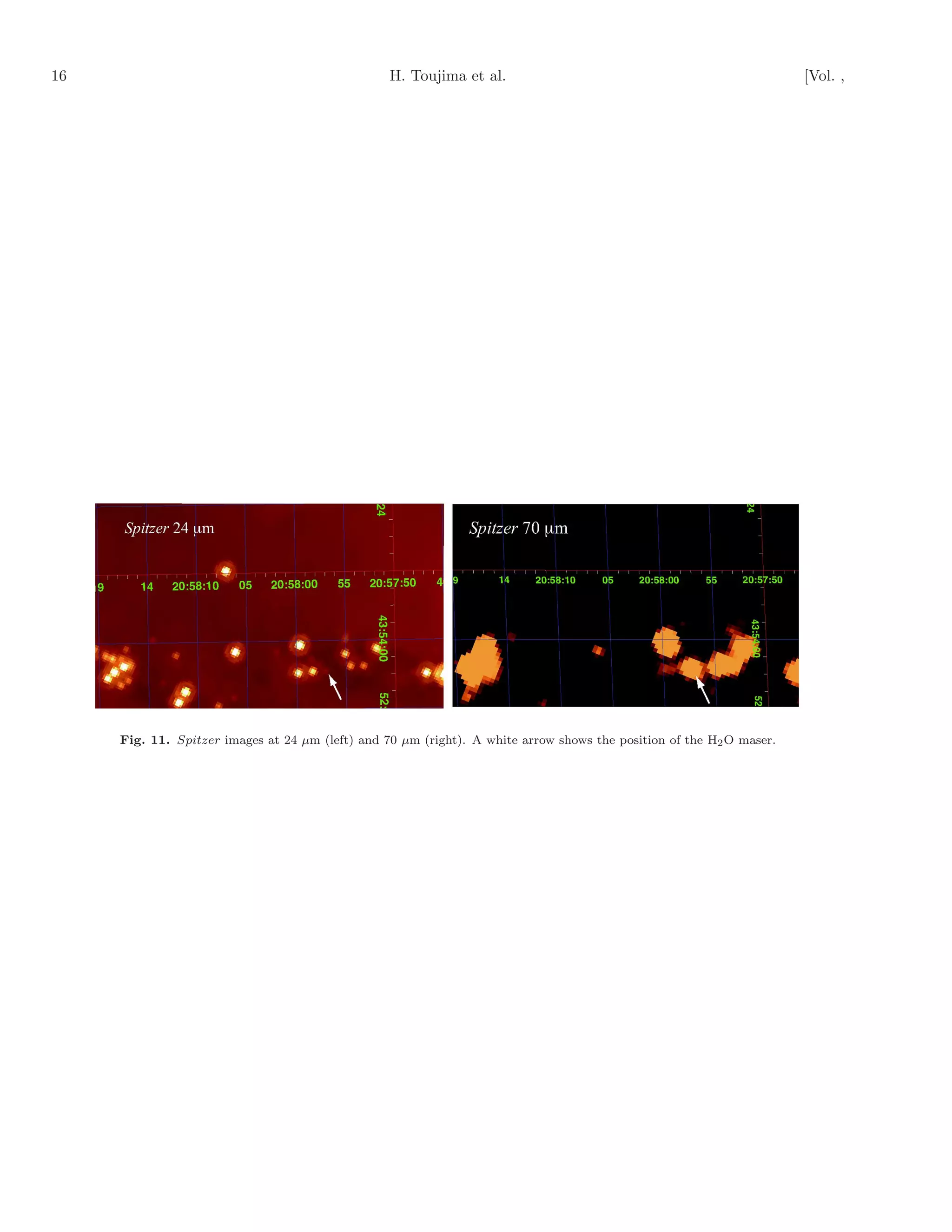
of some sources. Figure 15 shows an IRAS image at 100 132
µm overlayed on our NH3 map. A complex source is found Cambr´sy, L., Beichman, C. A., Jarrett, T. H., & Cutri, R. M.
e
near clump-A in the IRAS image, although it is composed 2002, AJ, 123, 2559
of several infrared sources in the Spitzer image (see Figure Chandler, C. J., & Carlstrom, J. E. 1996, ApJ, 466, 338
Claussen, M. J., Wilking, B. A., Benson, P. J., Wootten, A.,
11).
Myers, P. C., & Terebey, S. 1996, ApJS, 106, 111
This suggests that there are many H2 O maser sources Codella, C., Welser, R., Henkel, C., Benson, P. J., & Myers,
which are not catalogued in the IRAS PSC. A new H2 O P. C. 1997, A&A, 324, 203
maser survey should be carried out based on a point source Cohen, M., & Kuhi, L. V. 1979, ApJS, 41, 743
catalogue with a higher resolution and sensitivity, such asq Comer´n, F., & Pasquali, A. 2005, A&A, 430, 541
o
Spitzer and/or AKARI should be carried out. Our new Dahm, S. E., & Simon, T. 2005, AJ, 129, 829
H2 O maser is associated with a far-infrared source, and Danby, G., Flower, D. R., Valiron, P., Schilke, P., & Walmsley,
its luminosity is brighter than that of the mid-infrared. C. M. 1988, MNRAS, 235, 229
This characteristic may be a good criterion with which to Deharveng, L., Lefloch, B., Zavagno, A., Caplan, J.,
find new H2 O maser sources. Whitworth, A. P., Nadeau, D., & Mart´ S. 2003, A&A,
ın,
408, L25
Deharveng, L., Zavagno, A., & Caplan, J. 2005, A&A, 433,
5. Conclusions 565
Dobashi, K., Bernard, J.-P., Yonekura, Y., & Fukui, Y. 1994,
We observed NGC 7000 in the NH3 line and H2 O maser ApJS, 95, 419
using the Kashima 34-m telescope. Our observations are Dobashi, K., Yonekura, Y., Matsumoto, T., Momose, M., Sato,
summarized as follows: F., Bernard, J.-P., & Ogawa, H. 2001, PASJ, 53, 85
Duerr, R., Imhoff, C. L., & Lada, C. J. 1982, ApJ, 261, 135
1. We found two major clumps with a mass of 95–452 Evans, N. J., et al. 2009, ApJS, 181, 321
M⊙ , and three subclumps with a mass of 9–20 M⊙ . Fountain, W. F., Gary, G. A., & Odell, C. R. 1983, ApJ, 269,
The molecular gas in these show similar gas kinetic 164
temperatures of 11–15 K and line width of 1–2 km Furuya, R. S., Kitamura, Y., Wootten, A., Claussen, M. J., &
s−1 . However, they show different star formation Kawabe, R. 2003, ApJS, 144, 71
activities such as the concentration of T-Tauri type Genzel, R., Ho, P. T. P., Bieging, J., & Downes, D. 1982,
stars and the association of an H2 O maser. ApJL, 259, L103
2. One of the clumps that is associated with a cluster of Herbig, G. H. 1958, ApJ, 128, 259
T-Tauri type stars shows the SFE ≃ 36–62%. This Ho, P. T. P., & Townes, C. H. 1983, ARA&A, 21, 239
SFE is higher than that of the other clumps. Gandolfi, D., et al. 2008, ApJ, 687, 1303
Kun, M., Balog, Z., Kenyon, S. J., Mamajek, E. E., &
3. A comparison of the distribution of molecular gas Gutermuth, R. A. 2009, ApJS, 185, 451
and ionized gas traced by the Hα emission suggests Kutner, M. L., & Ulich, B. L. 1981, ApJ, 250, 341
that the clump with high SFE is located near the H II Lada, E. A. 1992, ApJL, 393, L25
region. Therefore, the high SFE would be related to Lada, E. A., Evans, N. J., II, & Falgarone, E. 1997, ApJ, 488,
the interaction of molecular gas and the H II region. 286
4. We found a new H2 O maser source in the NH3 Ladd, E. F., Myers, P. C., & Goodman, A. A. 1994, ApJ, 433,
clump. Although the counterpart of this maser is 117
not found in the IRAS point source catalogue, we Laugalys, V., & Straiˇys, V. 2002, Baltic Astronomy, 11, 205
z
found it in the Spitzer 24- and 70-µm images. This Lang, K. R., & Willson, R. F. 1980, ApJ, 238, 867
suggests that a new H2 O maser survey should be Leisawitz, D., Bash, F. N., & Thaddeus, P. 1989, ApJS, 70,
731
carried out based on the point source catalogue of
MacLaren, I., Richardson, K. M., & Wolfendale, A. W. 1988,
Spitzer and/or AKARI. ApJ, 333, 821
Matzner, C. D., & McKee, C. F. 2000, ApJ, 545, 364
We thank an anonymous referee for very useful com- Myers, P. C., & Benson, P. J. 1983, ApJ, 266, 309
ments and suggestions. T.O. was supported by a Grant- Myers, P. C., Dame, T. M., Thaddeus, P., Cohen, R. S.,
Silverberg, R. F., Dwek, E., & Hauser, M. G. 1986, ApJ,
in-Aid for Scientific Research from the Japan Society for
301, 398
the Promotion Science (17340055). We acknowledge K. Nakajima, T., et al. 2007, PASJ, 59, 1005

8. 8 H. Toujima et al. [Vol. ,
Prasad, S. S., & Huntress, W. T., Jr. 1980, ApJS, 43, 1
Ridge, N. A., Wilson, T. L., Megeath, S. T., Allen, L. E., &
Myers, P. C. 2003, AJ, 126, 286
Rieke, G. H., & Lebofsky, M. J. 1985, ApJ, 288, 618
Rohlfs, K., & Wilson, T. L. 1996, Tools of Radio Astronomy,
XVI, 423 pp. 127 figs., 20 tabs.. Springer-Verlag Berlin
Heidelberg New York. Also Astronomy and Astrophysics
Library,
Straiˇys, V., & Laugalys, V. 2008, Baltic Astronomy, 17, 143
z
Sugitani, K., Fukui, Y., Mizuni, A., & Ohashi, N. 1989, ApJL,
342, L87
Sugitani, K., Fukui, Y., & Ogura, K. 1991, ApJS, 77, 59
Sugitani, K., & Ogura, K. 1994, ApJS, 92, 163
Swift, J. J., & Welch, W. J. 2008, ApJS, 174, 202
Tieftrunk, A. R., Megeath, S. T., Wilson, T. L., & Rayner,
J. T. 1998, A&A, 336, 991
Ungerechts, H., Walmsley, C. M., & Winnewisser, G. 1980,
A&A, 88, 259
Ungerechts, H., Winnewisser, G., & Walmsley, C. M. 1982,
A&A, 111, 339
Walborn, N. R. 2007, arXiv:astro-ph/0701573
Walmsley, C. M., & Ungerechts, H. 1983, A&A, 122, 164
Wendker, H. J. 1984, A&AS, 58, 291

9. No. ] NH3 and H2 O maser emissions in NGC 7000 9
Table 1. Line parameters obtained at the peak position of the clumps and the subclumps
Clump R.A. Decl. Line TMB ∗ vLSR † ∆v † TMB dv ‡ rms noise
(J2000) (J2000) (J, K) (K) (km s−1 ) (km s−1 ) (K km s−1 ) (K)
A1 20h 58m18. 8
s
+43◦53′ 24′′ (1,1) 1.92 5.6 1.5 2.96±0.13 0.10
(2,2) 0.43 5.0 1.2 0.55±0.15 0.11
(3,3) ≤0.30§ ··· ··· ··· 0.10
A2 20h 58m02. 1
s
+43◦53′ 24′′ (1,1) 2.59 5.5 1.4 3.85±0.09 0.07
(2,2) 0.56 5.4 1.6 0.93±0.11 0.08
(3,3) ≤0.21§ ··· ··· ··· 0.07
A3 20h 57m45. 5
s
+43◦53′ 24′′ (1,1) 1.44 5.3 2.1 3.21±0.13 0.08
(2,2) 0.38 5.0 2.7 1.11±0.12 0.08
(3,3) ≤0.24§ ··· ··· ··· 0.08
B 20h 56m49. 9
s
+43◦43′ 24′′ (1,1) 2.79 1.5 1.9 6.25±0.21 0.14
(2,2) 0.70 1.5 1.8 1.58±0.20 0.14
(3,3) ≤0.42§ ··· ··· ··· 0.14
∗ The error of the Gaussian fitting is close to the rms noise level.
† The error of the Gaussian fitting is much smaller than the velocity resolution (0.39 km s−1 ).
‡ The error corresponds to one standard deviation.
§ The upper limit is given as 3 times of the rms noise.
Table 2. Physical properties of the clumps and the subclumps
Clump Size τ(1,1) Trot N (NH3 ) MLTE Mvir
(pc) (K) (cm−2 ) (M⊙ ) (M⊙ )
A1 0.21 1.4±0.4 12±2 2.4×1015 12 ···
A2 0.31 1.2±0.3 13±1 1.8×1015 20 ···
A3 0.21 0.8±0.4 15±2 1.8×1015 9 ···
A 0.67 1.2±0.2 13±1 1.8×1015 95 125
B 1.02 1.6±0.2 11±1 3.7×1015 452 350
Table 3. Star formation efficiency of individual clumps
Clump Number of sources Stellar mass (M⊙ ) SFE (%)
T-Tauri Total T-Tauri Total T-Tauri Total
A1 5 < 15 6.9 < 19.9 36 < 62
A2 1 <5 0.8 < 6.0 4 < 23
A3 0 <4 0 < 5.2 0 < 36
A 7 < 32 7.7 < 41.5 8 < 30
B 0 < 24 0 < 31.2 0 <6

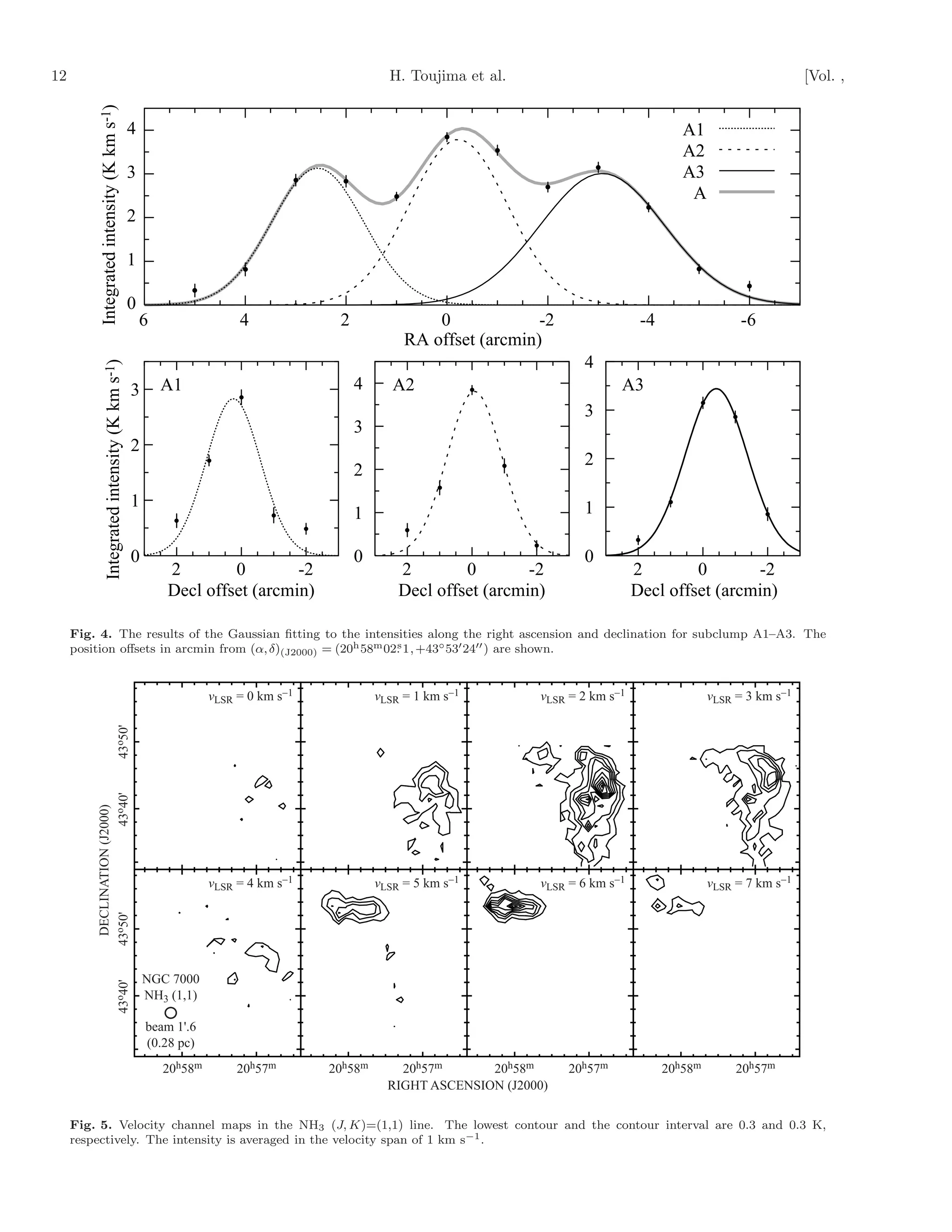
10. 10 H. Toujima et al. [Vol. ,
Fig. 1. Optical image of the W80 region (CalTech/Palomar) that comprises two H II regions of NGC 7000 (North Amrica nebula)
and IC 5070 (Pelican nebula) and dark lanes of L935. Yellow crosses show the positions of T-Tauri type stars (Herbig 1958). A blue
cross shows the position of an O5 V type star (Comer´n & Pasquali 2005).
o
Main beam temperature [K]
3
A1 A2 A3 B
2 (+3,0) (0,0) (-3,0) (-13,-10)
(J,K)=(1,1)
1
0
(J,K)=(2,2)
-20 0 20 -20 0 20 -20 0 20 -20 0 20
LSR velocity [km s-1]
Fig. 2. Spectra in the NH3 (J, K)=(1,1) and (2,2) lines observed at the peak position of the subclumps and the clump-B. The
position offsets in arcmin from (α, δ)(J2000) = (20h 58m 02. 1, +43◦ 53′ 24′′ ) are shown in the top-right corner.
s

11. No. ] NH3 and H2 O maser emissions in NGC 7000 11
NGC 7000
A NH3 (1,1)
A1
43o50'
A2 A3
DECLINATION (J2000)
B
43o40'
l b
beam 1'.6
(0.28 pc)
20h58m 20h57m
RIGHT ASCENSION (J2000)
Fig. 3. Integrated intensity map of the main hyperfine component of the NH3 (1,1) line. The lowest contour and the contour
interval are 0.3 and 0.6 K km s−1 , respectively. The circle in the bottom-left corner shows the beam size. The gray ellipses show
the extents of the clumps and the subclumps. The triangles and squares show the T-Tauri stars and MSX sources, respectively. The
cross shows the position of the H2 O maser. The dashed line shows the axis of the position velocity map shown in Figure 6.

12. 12 H. Toujima et al. [Vol. ,
Integrated intensity (K km s-1)
4 A1
A2
3 A3
A
2
1
0
6 4 2 0 -2 -4 -6
RA offset (arcmin)
4
Integrated intensity (K km s-1)
3 A1 4 A2 A3
3
3
2
2
2
1 1
1
0 0 0
2 0 -2 2 0 -2 2 0 -2
Decl offset (arcmin) Decl offset (arcmin) Decl offset (arcmin)
Fig. 4. The results of the Gaussian fitting to the intensities along the right ascension and declination for subclump A1–A3. The
position offsets in arcmin from (α, δ)(J2000) = (20h 58m 02. 1, +43◦ 53′ 24′′ ) are shown.
s
vLSR = 0 km s−1 vLSR = 1 km s−1 vLSR = 2 km s−1 vLSR = 3 km s−1
43o40' 43o50'
DECLINATION (J2000)
vLSR = 4 km s−1 vLSR = 5 km s−1 vLSR = 6 km s−1 vLSR = 7 km s−1
43o50'
NGC 7000
43o40'
NH3 (1,1)
beam 1'.6
(0.28 pc)
20h58m 20h57m 20h58m 20h57m 20h58m 20h57m 20h58m 20h57m
RIGHT ASCENSION (J2000)
Fig. 5. Velocity channel maps in the NH3 (J, K)=(1,1) line. The lowest contour and the contour interval are 0.3 and 0.3 K,
respectively. The intensity is averaged in the velocity span of 1 km s−1 .

13. No. ] NH3 and H2 O maser emissions in NGC 7000 13
8
7
6
A
LSR velocity [km s−1]
5
4
3
2
1 B
0
−1
+3 0 −3 −6 −9 −12 −15 −18
Position offset [arcmin]
Fig. 6. Position-velocity map of the whole cloud in the NH3 (J, K)=(1,1) line. The lowest contour and the contour interval are 0.2
and 0.2 K at the TMB unit, respectively. The position offset is relative to the position at (α, δ)(J2000) = (20h 58m 02. 1, +43◦ 53′ 24′′ )
s
along the dashed line shown in Figure 3.
velocity gradient velocity gradient
0.32 +/− 0.03 km s−1 arcmin−1 0.48 +/− 0.08 km s−1 arcmin−1
1.8 +/− 0.2 km s−1 pc−1 2.8 +/− 0.5 km s−1 pc−1
8
A3 peak 4 B peak
LSR Velocity [km s -1]
LSR Velocity [km s -1]
7
3
6
2
5 1
4 0
3 -1
+4 +2 0 -2 -4 +3 +2 +1 0 -1 -2 -3
Position offset [arcmin] Position offset [arcmin]
Fig. 7. Position-velocity maps of the NH3 (J, K)=(1,1) line toward subclump-A3 (left) and clump-B (right). The lowest contour
and the contour interval are 0.3 and 0.3 K, respectively. The position offset is relative to the peak positions at (α, δ)(J2000) =
(20h 57m 45. 5, +43◦ 53′ 24′′ ) along the position angle of 45◦ for the A3 peak and (20h 56m 49. 9, +43◦ 43′ 24′′ ) along the position angle
s s
of 90◦ for the B peak.

14. 14 H. Toujima et al. [Vol. ,
W main [K km s-1]
6 A1 : inner A2 : inner A3 : inner clump-A : inner clump-B : inner
5
4
3
2
1
0
0 1 2 3 0 1 2 3 0 1 20 3 1 2 3 0 1 2 3
W satellite [K km s-1]
W main [K km s-1]
6 A1 : outer A2 :outer A3 :outer clump-A : outer clump-B : outer
5
4
3
2
1
0
0 1 2 3 0 1 2 3 0 1 2 0 3 1 2 3 0 1 2 3
W satellite [K km s -1]
Fig. 8. Correlations of the integrated intensity in the (1,1) main and satellite lines. The correlations of the main to the inner and
outer satellite lines are shown in the top and bottom panel, respectively. The data detected over the 3 σ level in both the main and
the satellite lines are plotted. The error bar shows the rms noise (1σ). The estimated optical depth is shown in the bottom of each
panel.
WNH3(2,2) [K km s-1]
sub-clump A1 sub-clump A2 sub-clump A3 clump A clump B
2 R(2,2)/(1,1) = 0.18 +- 0.05 R(2,2)/(1,1) = 0.22 +- 0.03 R(2,2)/(1,1) = 0.29 +- 0.05 R(2,2)/(1,1) = 0.24 +- 0.02 R(2,2)/(1,1) = 0.18 +- 0.02
Trot = 12 +- 2 K Trot = 13 +- 1 K Trot = 15 +- 2 K Trot = 13 +- 1 K Trot = 11 +- 1 K
1
0
0 1 2 3 4 5 6 0 1 2 3 4 5 6 0 1 2 3 4 5 6 0 1 2 3 4 5 6 0 1 2 3 4 5 6
WNH3(1,1) [K km s-1]
Fig. 9. Correlations of the integrated intensity in the (1,1) and (2,2) lines. The data detected over the 3 σ level in both the (1,1)
and the (2,2) lines are plotted. The error bar shows the rms noise (1σ). The estimated Trot is shown in each panel.

15. No. ] NH3 and H2 O maser emissions in NGC 7000 15
30 2007 Aug 21
20
10
0
90
2007 Sep 25
60
30
0
60 2007 Oct 31
40
20
0
80
2007 Nov 23
60
40
20
0 8.4 km s−1
120
Flux density [Jy]
2007 Dec 27
80
40
0
90
2008 Jan 28
60
30
0 9.0 km s−1
20 2008 Apr 22
10
0
10 2008 May 05
5
0 9.6 km s−1
10 2008 Oct 02
5
0
7 8 9 10 11
LSR veocity [km s−1]
Fig. 10. H2 O maser spectra obtained by our single-dish monitoring observations. Two velocity jumps are found between November
and December of 2007, and between January and April of 2008. The maser emission disappeared in October 2008.

16. 16 H. Toujima et al. [Vol. ,
Fig. 11. Spitzer images at 24 µm (left) and 70 µm (right). A white arrow shows the position of the H2 O maser.

17. No. ] NH3 and H2 O maser emissions in NGC 7000 17
2
counterpart of class I
10 the H2O maser
in A2
class 0
1 class II
10 -2
-4 T = 44 K
10 L = 42 LÍ
2 G085.0482-01.1330
10 in A3
Flux density [Jy]
1
-2
10
-4 T = 130 K
10 L = 190 LÍ
2 G084.8235-01.1094
10 in B
1
-2
10
-4
T = 130 K
10 L = 230 LÍ
10 -7 10 -6 10 -5 10 -4 10 -3
Wavelength [m]
Fig. 12. Spectral energy distribution of the three infrared sources. The solid line shows the best fit blackbody with parameters
shown at the right-bottom corner in each panel. The gray dashed lines in the top panel show typical spectra of class 0, I, and II
(Bachiller 1996).

18. 18 H. Toujima et al. [Vol. ,
45o00'
DECLINATION (J2000)
44o30'
44o00'
43o30'
(a)
21h00m 20h58m 20h56m 20h54m 20h52m 20h50m 20h48m
RIGHT ASCENSION (J2000)
−6 −4 −2 0 2 4 6 8 10 12 14
LSR velocity [km s−1]
45o00'
DECLINATION (J2000)
44o30'
44o00'
43o30'
(b)
21h00m 20h58m 20h56m 20h54m 20h52m 20h50m 20h48m
RIGHT ASCENSION (J2000)
12 15 18 21 24 27 30 33 36 39 42
FWHM [km s−1]
Fig. 13. (a) The LSR velocity map of the H α emission (color; Fountain et al. 1983) on which the 13 CO integrated intensity map
(black contour; Dobashi et al. 1994) and the NH3 (1,1) integrated intensity map (red contour) are superimposed. The black cross
is the emission line star (Herbig 1958). (b) The FWHM map of the H α emission (color; Fountain et al. 1983) superimposed on the
same maps as that shown in (a).

19. No. ] NH3 and H2 O maser emissions in NGC 7000 19
Fig. 14. Schematic geometry of the NH3 clumps and the H II region.
Fig. 15. IRAS 100 µm image (gray scale) on which the integrated intensity map of NH3 (1,1) line (contour) is superimposed.