This document presents carpet plots generated using MATLAB for a laminate composed of 8 layers with different orientations. The plots show: 1. The in-plane modulus Ex versus thickness fraction for +/- 45 degree layers. 2. The in-plane Poisson's ratio versus thickness fraction for +/- 45 degree layers. 3. The shear modulus Gxy versus thickness fraction for +/- 45 degree layers. 4. The bending modulus Exb versus thickness fraction for +/- 45 degree layers. 5. The Poisson's ratio in bending vxy_b versus thickness fraction for +/- 45 degree layers. The plots match those in the reference textbook, verifying the MATLAB code used to generate the carpet plots.

1. Fourth Year Composite materials
Report: Project final ((Carpet plots))
Report No: final Date: 21/5/2013
Submitted to: Dr. Mohammad Tawfik
Name
 Mohammad Tawfik Eraky
‫عراقي‬ ‫أحمد‬ ‫توفيق‬ ‫محمد‬
2013/2014

2. 2
Contents
Carpet plots.....................................................................................................................................................................4
Laminate..........................................................................................................................................................................4
1. Carpet plot for laminate in plane modulus Ex under inplane load Nx...............................................................4
2. Carpet plot for laminate in plane poisson ratio in x-y plan.................................................................................6
3. Carpet plot for laminate shear modlus Gxy under in plane load in x-y plan ....................................................8
4. Carpet plot for laminate bending modulus Exb under in plane load in x-y plan ..............................................9
5. Carpet plot for inplane poisson ratio v_xy bending modulus Exb under in plane load in x-y plan................11
APPENDEX .....................................................................................................................................................................13
MATLAB program code ............................................................................................................................................13
Table of figures
Figure 1 Ex versus thickness fraction gamma .................................................................................................................4
Figure 2 poisson ratio versus thickness fraction of lamina +45/-45...............................................................................6
Figure 3 shear modlus vs gamma....................................................................................................................................8
Figure 4 bending modulus versus thickness ratio...........................................................................................................9
Figure 5 poisson ratio in bending loading Exb .............................................................................................................11

3. 3
Introduction
The analysis of deformation of laminated composites can be done accurately, once the orientations ,laminate total thickness
have been chosen ,however the analysis methodology presented so far doesn’t indicate how to design the laminate; that is ,it
doesn’t provide a simple procedure to estimate the required thickness ,layer orientations, ideally the designer would like to
follow a procedure ,which starting with the load and the boundary conditions leads to the complete preliminary design of the
laminate .A laminate design consists of material, number of layers ,layer thickness and orientations ,laminate stacking sequence.
The material specification includes resin and fiber types, fiber volume fraction, and fiber architecture in various layers
Most engineers have considerable training and experience in the design of simple structure components, laminate moduli can be
used to take the advantage of this knowledge for the design of the composite structures.
To simplify the design process ,plots of apparent moduli for various laminate configuration can be produced before hand

4. 4
Carpet plots
Carpet plots are constructed for a specific material type and fiber volume fraction, E-glass and isophthalic
polyester matrix with VF =0.5 have been used to construct the carpet plots in figures, using in
plane loading relations
Laminate
We used laminate composed of 8 laminas symmetric, with the following
Lamina Orientation
 0/90/45/-45/-45/45/90/0.
By constructing a MATLAB code, we generate the following carpet plots, we compare the plots with that in
ch.6 in Barbero Introduction to composite materials , as verification
The MATLAB code attached in the appendix
1. Carpet plot for laminate in plane modulus Ex under inplane load Nx.
Figure 1 Ex versus thickness fraction gamma

5. 5
Comparing by barbero
We see that the plots are nearly identical

6. 6
2. Carpet plot for laminate in plane poisson ratio in x-y plan
Poisson ratio ranges from 0.1 to 0.6 as the thickness ratio for laminas changes
Figure 2 poisson ratio versus thickness fraction of lamina +45/-45

7. 7
Comparing by barbero

8. 8
3. Carpet plot for laminate shear modlus Gxy under in plane load in x-y plan
The shear modulus is directly affected by thickness ratio
Figure 3 shear modlus vs gamma

9. 9
4. Carpet plot for laminate bending modulus Exb under in plane load in x-y plan
If we have a lOOk at barber experimental results it’s not nearly the same but still good margin
Figure 4 bending modulus versus thickness ratio

10. 10
Barbero Results

11. 11
5. Carpet plot for inplane poisson ratio v_xy bending modulus Exb under in plane load in x-y plan
Figure 5 poisson ratio in bending loading Exb

12. 12
Barbero plots
We note that the MATLAB plots and BARBERO originate from 0.1,0.3 and ends at 0.6 so the
experimental results verified our Plots

13. 13
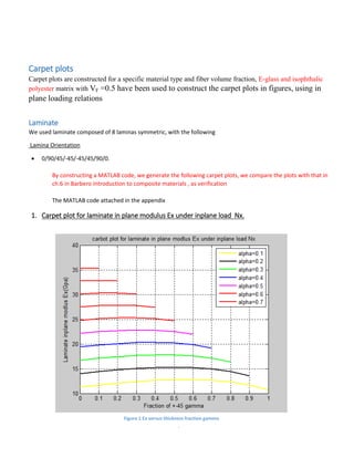
APPENDEX
MATLAB program code
clc;clear all;close all ;
%% material properities used [ E-glass and isophatalic-polyster matrix with vf=0.5 for
inplane loading]
t=16; %total thickness of the laminate
e_1=37.9 ; % longitinal modlus Gpa
e_2=11.3 ; %transverse modlus Gpa
g_12=3.3 ; % inplane shear modlus Gpa
new_12=0.3 ;% poisson ratio
v_f=0.5 ; % fiber volume ratio
new_21=new_12*e_2/e_1;
delta=1-new_12*new_21;
%% orientations %in rad
ceta_1=0;
ceta_2=90*pi/180;
ceta_3=45*pi/180;
ceta_4=-45*pi/180;
ceta_5=ceta_4;
ceta_6=ceta_3;
ceta_7=ceta_2;
ceta_8=ceta_1;
%% Q matrix
q=[e_1/delta new_12*e_2/delta 0;
new_12*e_2/delta e_2/delta 0;
0 0 2*g_12];
%% Transformation matrix
t1=[cos(ceta_1)^2 sin(ceta_1)^2 2*sin(ceta_1)*cos(ceta_1);
sin(ceta_1)^2 cos(ceta_1)^2 -2*sin(ceta_1)*cos(ceta_1);
-sin(ceta_1)*cos(ceta_1) sin(ceta_1)*cos(ceta_1) cos(ceta_1)^2-sin(ceta_1)^2];
t2=[cos(ceta_2)^2 sin(ceta_2)^2 2*sin(ceta_2)*cos(ceta_2);
sin(ceta_2)^2 cos(ceta_2)^2 -2*sin(ceta_2)*cos(ceta_2);
-sin(ceta_2)*cos(ceta_2) sin(ceta_2)*cos(ceta_2) cos(ceta_2)^2-sin(ceta_2)^2];
t3=[cos(ceta_3)^2 sin(ceta_3)^2 2*sin(ceta_3)*cos(ceta_3);
sin(ceta_3)^2 cos(ceta_3)^2 -2*sin(ceta_3)*cos(ceta_3);
-sin(ceta_3)*cos(ceta_3) sin(ceta_3)*cos(ceta_3) cos(ceta_3)^2-sin(ceta_3)^2];
t4=[cos(ceta_4)^2 sin(ceta_4)^2 2*sin(ceta_4)*cos(ceta_4);
sin(ceta_4)^2 cos(ceta_4)^2 -2*sin(ceta_4)*cos(ceta_4);
-sin(ceta_4)*cos(ceta_4) sin(ceta_4)*cos(ceta_4) cos(ceta_4)^2-sin(ceta_4)^2];
t5=t4; t6=t3 ; t7=t2; t8=t1;
%% Q matrices inverse

14. 14
t1_inv=inv(t1) ; t2_inv=inv(t2); t3_inv=inv(t3);t4_inv=inv(t4);t5_inv=t4_inv;
t6_inv=t3_inv;t7_inv=t2_inv; t8_inv=t1_inv;
%% Q-Bar matrices
q1_bar=(t1_inv)*q*t1; q2_bar=(t2_inv)*q*t2; q3_bar=(t3_inv)*q*t3;
q4_bar=(t4_inv)*q*t4;q5_bar=(t5_inv)*q*t5;
q6_bar=(t6_inv)*q*t6;q7_bar=(t7_inv)*q*t7;q8_bar=(t8_inv)*q*t8;
%% thickness calculations
alpha=0:0.1:1;
for i=1:length(alpha);
gamma=0:0.1:(1-alpha(i));
for j=1:length(gamma);
for n=1:length(alpha);
beta(n)=1-gamma(j)-alpha(i);
tl0=alpha(i)*t/2; tl90=beta(n)*t/2; tl45=gamma(j)*t/4;
%% Z-axis
z0=-t/2; z1=z0+tl0 ;z2=z1+tl90
;z3=z2+tl45;z4=z3+tl45;z5=z4+tl45;z6=z5+tl45;z7=z6+tl90;z8=z7+tl0;
%% A-matrix
A=q1_bar*tl0 + q2_bar*tl90+q3_bar*tl45 + q4_bar*tl45 +q5_bar*tl45 +q6_bar*tl45
+q7_bar*tl90 +q8_bar*tl0;
%%B-matrix
B=0.5*(q1_bar*(z1^2-z0^2)+q2_bar*(z2^2-z1^2) + q3_bar*(z3^2-z2^2) + q4_bar*(z4^2-z3^2)
+q5_bar*(z5^2-z4^2) + q6_bar*(z6^2-z5^2) + q7_bar*(z7^2-z6^2)+ q8_bar*(z8^2-z7^2));
%% D-matrix
D=(1/3)*(q1_bar*(z1^3-z0^3)+q2_bar*(z2^3-z1^3) + q3_bar*(z3^3-z2^3) + q4_bar*(z4^3-
z3^3) +q5_bar*(z5^3-z4^3) + q6_bar*(z6^3-z5^3) + q7_bar*(z7^3-z6^3)+ q8_bar*(z8^3-
z7^3));
%% EX
ex(j,n,i)=(A(1,1)*A(2,2)-A(1,2)*A(1,2))/(t*A(2,2));
%% new_xy
new_xy(j,n,i)=A(1,2)/A(2,2);
%% Lamina Shear modlus G_XY
g_xy(j,n,i)=A(3,3)/t;
%% EX-B
ex_b(j,n,i)=(12/t^3)*(D(1,1)*D(2,2)-D(1,2)^2)/D(2,2);
%%
vxy_b(j,n,i)=D(1,2)/D(2,2);
end
end
end
gamma=0:0.1:1;

15. 15
for i=1:length(alpha)
C = {'y','k','g','b','m','r','r','r','r','r','r'};
plot(gamma(1:(-i+1+length(gamma))),ex(1:(-
i+1+length(gamma)),1,i),'color',C{i},'linewidth',1.5),
legend({'alpha=0.1';'alpha=0.2
';'alpha=0.3';'alpha=0.4';'alpha=0.5';'alpha=0.6';'alpha=0.7'});grid on
ylabel('Laminate inplane modlus Ex(Gpa)');xlabel('Fraction of +-45 gamma');
title('carpet plot for laminate in plane modlus Ex under inplane load Nx');grid
on,hold on
end
figure
for i=1:length(alpha)
C = {'y','k','g','b','m','r','r','r','r','r','r'};
plot(gamma(1:(-i+1+length(gamma))),new_xy(1:(-
i+1+length(gamma)),1,i),'color',C{i},'linewidth',1.5),
legend({'alpha=0.1';'alpha=0.2
';'alpha=0.3';'alpha=0.4';'alpha=0.5';'alpha=0.6';'alpha=0.7'});grid on
ylabel('Laminate poisson ratio v_xy');xlabel('Fraction of +-45 gamma');
title('carpet plot for laminate in plane poisson ratio new_xy');grid on,hold on
end
figure
for i=1:length(alpha)
plot(gamma(1:(-i+1+length(gamma))),g_xy(1:(-
i+1+length(gamma)),1,i),'m','linewidth',1.5)
ylabel('Laminate shear modlus modlus Gx(Gpa)');xlabel('Fraction of +-45 gamma');
title('carpet plot for laminate shear modlus Gxy under inplane load Nxy');grid on
;hold on
end
figure
for i=1:length(alpha)
C = {'y','k','g','b','m','r','r','r','r','r','r'};
plot(gamma(1:(-i+1+length(gamma))),ex_b(1:(-
i+1+length(gamma)),1,i),'color',C{i},'linewidth',1.5),
legend({'alpha=0';'alpha=0.1';'alpha=0.2';'alpha=0.3';'5alpha=0.4';'alpha=0.5';'alpha=
0.6'});grid on
ylabel('Laminate bending modlus Exb(Gpa)');xlabel('Fraction of +-45 gamma');
title('carpet plot for laminate bending modlus Exb under ');grid on ;hold on
end
figure
for i=1:length(alpha)
C = {'y','k','g','b','m','r','r','r','r','r','r'};
plot(gamma(1:(-i+1+length(gamma))),vxy_b(1:(-
i+1+length(gamma)),1,i),'color',C{i},'linewidth',1.5),
legend({'alpha=0';'alpha=0.1';'alpha=0.2';'alpha=0.3';'5alpha=0.4';'alpha=0.5';'alpha=
0.6'});grid on
ylabel('Vxy_b');xlabel('raction of +-45 gamma');
title('carpet plot for inplane poisson ratio vxy_b in bending loadin modlus Exb
unde)');grid on ;hold on
end