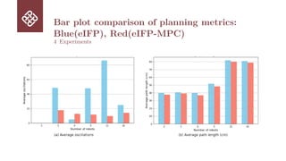
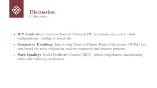
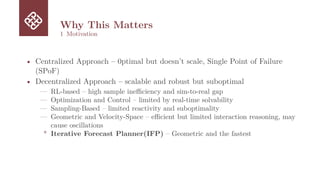
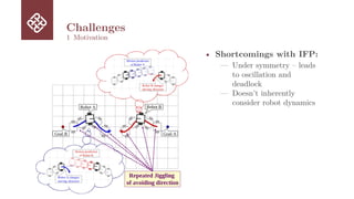
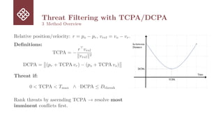
The 8th International Conference on Intelligent Robotics and Control Engineering, Kunming China, August 18-21, 2025 Abstract The Iterative Forecast Planner (IFP) is a geometric planning approach that offers lightweight computations, scalable, and reactive solutions for multi-robot path planning in decentralized, communication-free settings. However, it struggles in symmetric configurations, where mirrored interactions often lead to collisions and deadlocks. We introduce eIFP-MPC, an optimized and extended version of IFP that improves robustness and path consistency in dense, dynamic environments. 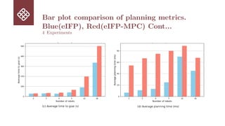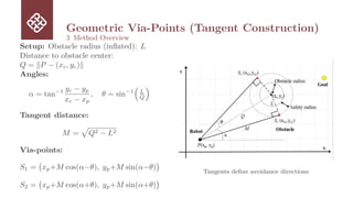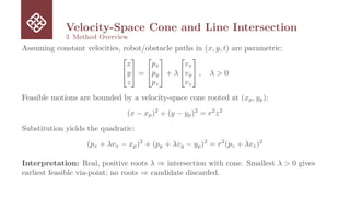The method refines threat prioritization using a time-to-collision heuristic, stabilizes path generation through cost-based via-point selection, and ensures dynamic feasibility by incorporating model predictive control (MPC) into the planning process. These enhancements are tightly integrated into the IFP to preserve its efficiency while improving its adaptability and stability. Extensive simulations across symmetric and high-density scenarios show that eIFP-MPC significantly reduces oscillations, ensures collision-free motion, and improves trajectory efficiency. The results demonstrate that geometric planners can be strengthened through optimization, enabling robust performance at scale in complex multi-agent environments. Paper: https://arxiv.org/abs/2508.08264

1. Forecast-Driven MPC for Decentralized
Multi-Robot Collision Avoidance
Hadush Hailu, Bruk Gebregziabher and Prudhvi Raj
IRCE 2025, Kunming
19 August 2025

2. Table of Contents
1 Motivation
▶ Motivation
▶ Contributions
▶ Method Overview
▶ Experiments
▶ Discussion

3. Why This Matters
1 Motivation
• Centralized Approach – 0ptimal but doesn’t scale, Single Point of Failure
(SPoF)
• Decentralized Approach – scalable and robust but suboptimal
— RL-based – high sample inefficiency and sim-to-real gap
— Optimization and Control – limited by real-time solvability
— Sampling-Based – limited reactivity and suboptimality
— Geometric and Velocity-Space – efficient but limited interaction reasoning, may
cause oscillations
* Iterative Forecast Planner(IFP) – Geometric and the fastest

4. Challenges
1 Motivation
• Shortcomings with IFP:
— Under symmetry – leads
to oscillation and
deadlock
— Doesn’t inherently
consider robot dynamics

5. Table of Contents
2 Contributions
▶ Motivation
▶ Contributions
▶ Method Overview
▶ Experiments
▶ Discussion

6. Forecast-Driven, Decentralized MPC
2 Contributions
Contributions
• TCPA (Time-to-Collision based) obstacle ranking
• Cost-function for via-point(global path) evaluation (not only the shortest)
• Integration with MPC

7. Table of Contents
3 Method Overview
▶ Motivation
▶ Contributions
▶ Method Overview
▶ Experiments
▶ Discussion

8. System Overview - Avoidance Direction(2D)
3 Method Overview

9. System Overview - Configuration Space(3D)
3 Method Overview

10. Robot Model
(Discrete unicycle dynamics)
3 Method Overview
State xk = [x, y, θ]⊤
, control uk = [v, ω]⊤
, ∆t sampling:
xk+1 =


xk + vk cos θk ∆t
yk + vk sin θk ∆t
θk + ωk ∆t

 , v ∈ [vmin, vmax], ω ∈ [ωmin, ωmax]

11. System Overview - Avoidance Direction(2D)
3 Method Overview

12. Threat Filtering with TCPA/DCPA
3 Method Overview
Relative position/velocity: r = po − pr, vrel = vo − vr.
Definitions:
TCPA = −
r⊤
vrel
∥vrel∥2
DCPA = (pr + TCPA vr) − (po + TCPA vo)
Threat if:
0 < TCPA < Tmax ∧ DCPA ≤ Dthresh
Rank threats by ascending TCPA → resolve most
imminent conflicts first.

13. Geometric Via-Points (Tangent Construction)
3 Method Overview
Setup: Obstacle radius (inflated): L
Distance to obstacle center:
Q = ∥P − (xc, yc)∥
Angles:
α = tan−1 yc − yp
xc − xp
, θ = sin−1
L
Q
Tangent distance:
M =
p
Q2 − L2
Via-points:
S1 = xp+M cos(α−θ), yp+M sin(α−θ)
S2 = xp+M cos(α+θ), yp+M sin(α+θ)
Tangents define avoidance directions

14. Velocity-Space Cone and Line Intersection
3 Method Overview
Assuming constant velocities, robot/obstacle paths in (x, y, t) are parametric:


x
y
z

 =


px
py
pz

 + λ


vx
vy
vz

 , λ 0
Feasible motions are bounded by a velocity-space cone rooted at (xp, yp):
(x − xp)2
+ (y − yp)2
= r2
z2
Substitution yields the quadratic:
(px + λvx − xp)2
+ (py + λvy − yp)2
= r2
(pz + λvz)2
Interpretation: Real, positive roots λ ⇒ intersection with cone. Smallest λ 0 gives
earliest feasible via-point; no roots ⇒ candidate discarded.

15. Cost-Based Via-Point Selection
3 Method Overview
For candidates vi with goal g and ghost-paths
{sj, gghost
j }:
J(vi) = wg ℓi + wd
X
j
wj
dij
+ wa
X
j
wj ϕij
where
ℓi =
∥pr − vi∥ + ∥vi − g∥
∥pr − g∥ + ϵ
and
ϕij = 1 −
(vi − pr)⊤
(gghost
j − sj)
∥vi − pr∥ ∥gghost
j − sj∥
.
Select v∗
= arg minvi J(vi) and discard candidates
too close to ghost paths.
Illustration cost based path evaluation

16. Trajectory Smoothing MPC Tracking
3 Method Overview
After selecting a via-point, the robot smooths waypoints and tracks them with MPC.
Spline Smoothing:
p(t) =
Sx(t)
Sy(t)
, t ∈ [0, 1]
Continuous cubic splines {Sx, Sy} provide positions derivatives.
Unicycle Dynamics:
xk+1 =


xk + vk cos θk ∆t
yk + vk sin θk ∆t
θk + ωk ∆t


MPC Optimization:
min
{uk}
N−1
X
k=0
∥xk − xref
k ∥2
Q + ∥uk∥2
R
subject to input bounds vmin ≤ vk ≤ vmax, ωmin ≤ ωk ≤ ωmax.
Predicted obstacles can be added as inequality constraints.

17. Table of Contents
4 Experiments
▶ Motivation
▶ Contributions
▶ Method Overview
▶ Experiments
▶ Discussion

18. Experimental Setup
4 Experiments
Scenarios
• Two-robot mirror
• 3-robot T and 120◦
• 4-robot cross
• 5-robot central converge
• 12-robot multi-directional
• 16-robot cross-flows

19. Experiments
4 Experiments

20. Experiments Cont...
4 Experiments

21. Quantitative comparison of planning methods
across setups
4 Experiments

22. Bar plot comparison of planning metrics:
Blue(eIFP), Red(eIFP-MPC)
4 Experiments

23. Bar plot comparison of planning metrics.
Blue(eIFP), Red(eIFP-MPC) Cont...
4 Experiments

24. Table of Contents
5 Discussion
▶ Motivation
▶ Contributions
▶ Method Overview
▶ Experiments
▶ Discussion

25. Discussion
5 Discussion
• IFP Limitation: Iterative Forcast Planner(IFP) fails under symmetric robot
configurations, leading to deadlocks.
• Symmetry Breaking: Introducing Time-to-Closest-Point-of-Approach (TCPA) and
cost-based via-point evaluation resolves symmetry and ensures progress.
• Path Quality: Model Predictive Control (MPC) refines trajectories, smoothening
paths and reducing oscillations.

26. Thank You
Questions welcome | had.hailu@gmail.com