SlideShare a Scribd company logo
1 of 165
Download to read offline
MODELING THE DYNAMIC RESPONSE OF THE
HUlMAN SPINE TO MECHANICAL SHOCK AND VIBRATION
      USING AN ARTIFICIAL NEURAL NETWORK


                    Jordan James Nicol
           B.A.Sc., Simon Fraser University, 1994


 THESIS SUBMITTED IN PARTIAL FULFILLMENT OF THE
        REQUIREMENTS FOR TIFIE CEGXEE OF
           MASTER OF APPLIED SCIENCE

            in the School of Engineering Science


             Copyright Jordan James Nicol1996
                 Simon Fraser Unversity
                        August 1996


              A l rights reserved. This work may not be
               l
            reproduced Irt whole or i part, by photocopy
                                     n
          or other means, without permission of the author.
Natronal Library                    Bibliotheque nationale
1+1 of Canada                           du Canada
        Acquisitions and                Direction des acquisitions et
        Bibliographic Services Branch   des services bibliographiques


                                                                        Your hle   Vorre reference


                                                                        Our file Nolre r.4lerence


 The author has granted an                              L'auteur a accorde une licence
 irrevocable non-exclusive licence                      irr&ocable et non exclusive
 allowing the National Library of                       permettant B la Bibliothbque
 Canada to reproduce, loan,                             nationale   du    Canada      de
 distribute or sell copies of                          reproduire, prgter, distribuer ou
 his/her thesis by any means and                       vendre des copies de sa these
 in any form or format, making                         de quelque maniere et sous
 this thesis available to interested                   quelque forme que ce soit pour
 persons.                                              mettre des exemplaires de cette
                                                       these a la disposition des
                                                       personnes interessees.


The author retains ownership of                        L'auteur conserve la propriete du
the copyright in his/her thesis.                       droit d'auteur qui protege sa
Neither the thesis nor substantial                     thhse. Ni la these ni des extraits
extracts from it may be printed or                     substantiels de celle-ci ne
otherwise reproduced without                           doivent &re       imprimes ou
his/her permission.                                    autrement reproduits sans son                 -
                                                       autorisation.
PARTIAL COPYRIGHT LICENSE


        I hereby grant to Simon Fraser University the right to lend my thesis,
project or extended essay (the title of which is shown below) to users of the
Simon Fraser University Library, and to make partial or single copies only for
such users or in response to a request from the library of any other university, or
other educational institution, on its own behalf or for one of its usrs. I further
agree that permission for multiple copying of this work for scholarly purposes
may be granted by E I ~ the Dean of Graduate Studies. It is understood that
                        or
copying or publication of this work for financial gain shall not be allowed without
my written permission.


Title of Thesis/PfojectlExtended Essay


"Modeling The Dynamic Response 0 6 The Human Spine To
Mechanical Shock And Vibration Using An Artificial Neurd
Network"


Author:
                       (signature)


                       July 25. 1996
                       (date)
Name:              Jordan James Nicol

Degree:            Master of Applied Science

Title of Thesis:   Modeling the dynamic response of the human spine to
                   mechanical shock and vibration using an artificial neural network


Examining Committee:


        CHAIR:            Dr. Shahram Payandeh


                          Dr. Andrew Rawicz
                          Senior Supervisor
                          School of Engineering Science


                             ames B. Morrison
                           mior Supervisor
                                  ~ i n e s i 6


                        7School of E     eering Science


                                          -

                         Dr. JohnJones
                         Internal Examiner
                         School of Engineering Science


                         Date Approved:
                                          F
The ability to model the spinal response to shock and vibration is an important step in

assessing the health hazard effects of repeated impacts to vehicle passengers. Current

methods used for this purpose, such as the Dynamic Response Index and the British

Standard 6841 filter, were found to perform poorly when the input consists of large-

magnitude shocks typical of those experienced by occupants of tanks, trucks, and other

off-road vehicles. In this thesis I present a novel approach to the problem of modeling

the spinal response of the seated passenger to vertical accelerations applied a t the seat.

The modeling approach taken utilizes an artificial neural network (ANN) to predict the

z-axis (vertical)acceleration at the fourth lumbar vertebra based on measured z-axis seat

acceleration. An ANN is a universal approximator, capable of modeling any continuous

function if trained with a sufficiently representative set of measured input-output data.

The seatspine system was modeled as a ~etwork
                                            with five inputs and one output. The

Levenberg-Marquardt algorithm was used to train the network by edjusting the

network parameters so as to minimize the square of the prediction error. The inputs to

the network are delayed samples of the measured inputs and predicted outputs of the

nonlinear simulation. It is shown that the trained network significantly outperforms

three different linear models examined for predicting the z-axis acceleration at the L-4

vertebra.
Dedicated to my parents, Ken and Marguerite,

 for their love, support, and encouragement.
The author wishes to thank Dr. James Morrison for his supervision and guidance
throughout this project. Recognition is also extended to Dr. Andrew Rawicz for his
consultation and assistance. Finally, special thanks to BC Research Inc, and the BC
Advanced Systems Institute for their financial support of this project.
CHAM'ER 2 HUMAN         RESPONSE I&&CNANIC~LSHOCK
                                             TO                                             AND VIBRATION ........................ 3
2.1 Mechanical Shock and Vibration in Vehicles ..................................................................... '2
2.2 Health Effects ........................................................................................................................  5
    2.2.1 Vertebral Efecfs............................................................................................................... 6
2.3 Existing Models....................................................................................................................... 9
2.4 Standards of Exposure ..................................................................................................                10

CHAPTER ARTIFICIAL
          3                        NEURAL          NETWORKS              .........................................................................   14
3.1 The Multi-Layer Perceptron................................................................................................                       17
3.2 Training ..................................................................................................................................      21
3.3 Steepest Descent Algorithms ............................................................................................                         22
3.4 Gauss-Newton Methods ......................................................................................................                      23
3.5 Generalization.......................................................................................................................            24

CHAPTERRECURRENT
          4               NEURAL            NETWORKS SYSTEM        FOR                      IDENTIECATION                    .................... 27
4.1 System Identification: Preliminary Concepts ................................................................... 27
    41.1 Inptif-Outpzlt Models ................................................................................................... 30
    4.1.2 Model Order...............................................................................................................              31
                   .                     . .
    4.1.3 The Eflects of Noise ..............        ...............  .                                               ........................... 32
                          Signals ................................................................................................. 34
    4.1.4 Clzoice of Inpt~f
4 2 Modeling Dynamical Systems with Recurrent Neural Networks................................ 35

CHAPTER METHODOLOGY
           5                           ..................................................................................................... 40
5.1 Statement of Problem........................................................................................................             40
5.2 Selection of Model Class .................................................................................................... 44
    5.2.1 Jusfficizfm for a nsrdimzr mode! ...................................................................... 4 4
                     i
    5.2.2 Jrrstification of the neural nefwork model ..................................................................... 47
5.3 Experiment...........................................................................................................................    48
    5.3.1 Data Processing for Model DeiieIopmmf..................................................................... 51
    5.3.2 Defemination of Training Subject and Trainingnesting Data ................................. 53
5.4 Selection of Model Structure .............................................................................................. 51
    5.4.1 Determinn tion oJMode1 Orders ................................................................................... 54
  - 5.4.2 Detevl~rim uf Hidden Lntjers .................................................................................. 56
                    tion
5.3 Parameter Estimation.......................................................................................................... 58
    5.5.1 m e Compromise Method ............................................................................................ 58
    5.5.2 The Leuenberg-Mnrqzinrdt Method .......................................................................... 59
-
3.6 Model Validation ................................................................................................................ h3

CHAPTER6 RESULTS       .................................................................................................................. 65
6.1 Determination of Subject Data ........................................................................................                65
6.2 Determination of Model Orders ........................................................................................ 66
6.3 Determination of the Number of Hidden Pes .................................................................                           68
6.4 Final Model Structure ......................................................................................................... h9
6.5 Mode! Validation .................................................................................................................    70
6.6 Model Comparisons............................................................................................................         76
    6.6.1 RNN Model .................................................................................................................. 76
    6.6.2 The Dynamic Response Index Model ........................................................................... 78
    6.6.3 The British Standard 6841 Filter .................................................................................. 80
    6.6.4 Auto-Regressive Model with Exogototls Inputs .......................................................... 82
6.7 Cross-Subject Validation..................................................................................................... 83
    6.7.1 Cross-Subject Validation of the Model's Xespoizse to Vibration ................................. 87

CHAPTER DISCUSSION
          7                       .........................................................................................................     9.1
7.1 Model Response to Positive Input Shocks ....................................................................... 94
7.2 Model Response to Negative Input Shocks ................................................................. 95
7.3 Cross-3ubject Validation Results....................................................................................... 95
7.4 Model Performance on Vibration ...................................................................................... 96
7.5 Model Limitations ...............................................................................................................           97
7.6 Stability ......................  .  ..................................................................................................... 700
7.7 Complexity/Iii~plementation                     Issues............................................................................... 103


APPENDIX MATLAB
          A           NEURAL           NETWORK             SCRIPT        FILES      ...................................................      l'l!?
A.l Training Routines .............................................................................................................          1'15
A.2 Validation Routines..........................................................................................................            '120
A.3 Neural Network Toolbox Functions ..............................................................................                          121


       D
APPENDIX THEARX MODEL LEAST
                    AND        ESTIMATION
                          SQUARES        ................................ 148

bPENDUC E &EU&ENTATION OF THE BS 6841 FILTERAND THE DRI MODEL.............. 151


                                                                        vii
Figure 2.1 The posterior and lateral views of the human spine.
Figure 2 2 Spinal Unit.
        .
Figure 2 3 Biodynarnic model used in Dynamic Response Index.
        .
Figure 24 Magnitude frequency response of the DRI model and the B
        .                                                        S
          6841 filter.
Figure 3 1 Biological Neuron.
        .
Figure 3.2 Multilayer Perceptron
Figure 3.3 Basic Processing Element.
Figure 3.4 M layer Perceptron
Figure 4 1 System identification approach.
        .
Figure 4 2 Time-delayed neural network.
        .
Figure 4.3 Externally-recurrent neural network.
Figure 4.4 Internally-recurrentneural network.
Figure 4 5 Fully-recurrent neural network.
        .
Figure 5.1 (a) Block diagram of the seat-spine system. (b) Degrees of
           freedom in terms of acceleration of the human body.
Figure 5 2 Simplified seat-spine system.
        .
Figure 5 3 System Identification Flowchart
        .
Figure 5 4 Peak transmission ratios for positive seat shocks.
        .
Figure 5 5 Peak transmission ratios for negative seat shocks.
        .
Figure 5 6 L4 response to 3g, 4Hz seat shock.
        .
Figure 5.7 L4 response to -3g, 4 3 3 seat shock.
Figure 5.8 lMARS table and subjeci.
Figure 5.9 Input shock waveform diagram.
Figure 6.1 The mean normalized power spectral density of the lumbar-4
           response.
Figure 6.2 Plot of the lag space for input-ouput data (m = 2)..
Figure 6.3 RMS error vs hidden PEs
Figure 6.4 RMS Error vs. trairing iterations.
Figure 6.5 hafized neurd network structure.
Figure 6.6 Response to Ig/5Hz, -Zg/5Hzf 3g/SHz input shocks.
Figure 67 Response to 4g/iliiz, -ig/3iiz, -2g/6Hz, i g / i l ! : i ~ ~ p u t
        .                                                      z
            shocks
Figure 6.8 Response to -3g/5Hz, 3g/ 15Hz1and 4g/8Hz input shocks
Figure 6.9 Response to -Ig/Wz, -4g/SHz, Ig/6Hz, and -3g/15Hz input
           shocks.
Figure 6.10 Response to 2g/5Hz, 4g/4Hzf -lg/6Hz input shocks.
Figure 6.11 Response to.-3g/6Hz, lg/llHz, and -2g/SHz input mocks.
Figure 6.12 Response to -2g/8Hz, 3g/20Hz1 and 3g/4Hz input shocks.
Figure 6.13 Response to - l g / W , -4g/5Hzl and lg/2Hz input shocks
Figure 6.14 Response to -2g/llHz, 2g/20Hz1 and 3g/15Hz input shocks
Figure 6.15 Response to.-3g/4Hz, and lg/2Hz input shocks.
Figure 6.25 Response to -2g/6=,     and 3g/4Hz input shocks.
Figure 6.17 Response to 4g/4Hz, -lg/8Hz and -4g/12Hz. input shocks.
Figure 6.18. Response to lg/l?Hz, -2g/8Hz, and 2g/4Hz input shocks.
Figure 6.19 Response to 4g/llHz, -Ig/ l5&, and -4g/8Hz input shocks.
Figure 6.20 Response to -2g/5Hz input shock.
Figure 6.21 Response to a 4g/4Hz input shock.
Figure 6.22 Response to a 3 g / W input shock.
Figure 6.23 Response to a -4g/5Hz input shock
Figure 6.24 Response to a 4g/llHz input shock
Figure 6.25 Response to a -2g/5Hz input shock.
Figure 6.26 Reponse to a 4g/&      input shock.
Figure 6.2'7 Response to a 3g/4& input shock.
Figure 6.28 Response to a -4g/5Hz input shock.
Figure 6.29 Response to a 4g/llHz input shock.
Figure 6.30 Response to a -2g/5Hz input shock.
Figure 6.31 Response to a 4g/4Hz input shock.
Fi,oure 6.32 Response to a 3g/4Hz input shock.
Figtire 6.33 Resporiie to a 4g/5& input shock.
Figure 6.34 Response to a 4g/llHz input shock.
Figure 6.35 Response to a -2g/5Hz input shock.
Figure 6.36 Response to a 4g/4Hz input shock.
Figure 6.37 Response to a 3gf4l-I~
                                  input shock.


 Fibure 6 3 Response to a 4g/llWz input shock.
         .9
 Figure 6 4 Neural network and measured response to a -2g/5Hz shock.
         .0
 Figure 6 4 Neural network and measured response to a 4g/&
         .1                                                              shock.
Figure 6 4 Neural network and measured response to a 3g/4 Hz shock.
        .2
Figure 6 4 Neural network and measured response to a -4g/5Hz shock.
        .3
Figure 6-44Neural network and measured response to a -3g/4Hz shock
Figure 6 4 Neural network and measwed response to a 4g/ll& shock.
        .5
Figure 6 4 Neural network ancl measured response to background
        .6
           vibration with an r m value of 0.5g.
Figure 6.47 BS 6841 filter and measured response to background
            vibrzticn with zn rms value of 0.5g.
Figure 6 4 DRI model and measured response to backgromd vibration
        .8
           with an rms value of 0.5g.
Figure 6 4 20'th order ARX model and measured response to
        .9
           background vibration with an m s value of 0.5g.
Figure 6 5 Power spectral density estimate of neural network and
        .0
           measured response to background vibration with an rlns
           value c 0.5g.
                  f
Figure 6.51 Power spectra! density estimate of DRI model and measured
            response to background vibration with an rms value of 0.5g.
Figure 6 5 Power spectral density estimate of BS 6841 and measured
        .2
           response to background vibration with an rms value of 0.5g.
Figure 6.53 Power spectral density estimate of 201thorder ARX model
            ancl measured (solid) response to background vibration with
            an rms value of 0.5g.
Figure 71 The neural network model response to impulses of log, 20g,
        .                                                                         101
           30g, and 40g
Figure 7.2 The neural network model response to impulses of -log, -20g1-          102
            30g, and -40g.
Figure 7.3 The neural rietwork model respome to impulses of 0.5g and -            102
            0.5g.
Figure F-12. Example of a free damped oscillation of the L4 acclererometer (z-    137
              axis) in response to perturbation of the skin.
Rgure F-13. Spectral density of a free damped oscillation of the skin-
             accelerometer system at L4 ( axis).
                                          z
Figure F-14. The high pass acceleration component of a skin perturbation.          13s
Figure F-15. The low pass acceleration component of a skin perturbation i          138
Figure F-16. The amplitsde components of low frequency and high frequency          139
               bone-skin transfer functions derived from a free damped
               oscillation. The cross-over frequency (fib was used to establish
               the cut-off frequency for low pass and high pass filtering of the
               measured acceleration signal.
Figure F-17 Recorded L4 accelerometer response to a -3 g, z axis shock at the      139
             seat and the predicted acceleration at the spinous process ilftcr
             correction by the skin transfer function.
Figure E.1 Error vs Model ozder for ARX model indentified using leas1              150
           squares estimation.


Table 5.1 Training data profile.
Table 5.2 Testing data profile.
Table 6.1 Similarity between subject and mean psd for various input shock
          responses, expressed as the normalized rrns error.
Table 6.2 Lipschitz number, q(nj for various ir'put lags (1) and output lags
           (m).
Table 6.3 Prediction errors for the few model types
TabIe 6.4 Prediction errors for the four model types for Subject 7.
Table 6.5 Time-domain prediction errors for the four model types for Subject
          7 in response to vibration.
Table 6.6 Frequency-domain prediction errors for the four model types for
          Subject 7 in response to vibration.
Table 7.1 Computational complexity of the vario~s
                                                models
Modeling physiological systems is an important tool in understanding how the human
 body operates and is affected by its environment. The complexity and nonlinear nature
 of living systems often makes the development of an accurate model difficult when
traditional linear modeling techniques are employed. In these circumstances, a
nonlinear modeling approach can yield a more accurate model, leading to a better
understanding of the real system.


A traditional modeling strategy is to develop the model strudure from first principles
and then to estimate the values of model coefficients from measured input and output
data. This analytical approach suffers if the system or process is either not well
understood or overly complex. I addition, the simplifymg assumptions upon which
                               n
the model is based may be incorrect under certain conditions. In many cases, linearity
is assumed over a certain operating range. The simplified system can then be
represented using a variety of welldeveloped linear modeling techniques. However, if
the nonlinearity is strong or a general model is required, a nonlinear modeling approach
is preferable.


One example of interaction between the human body and the environment is the case of
a seated passenger in a moving vehicle. I the vehicle travels over rough terrain the
                                        f
passenger's body will be subjected to a variety of motion-related stresses. For simplicity,
we can categorize these motion-related stresses as two distinct: phenomena: vibration
and mechanical shocks. For most of us, vehicle vibration and shocks are low magnitude
and infrequent, except for the occasional pothole. However, for passengers in rough-
terrain vehicles (tanks, mining and logging trucks, for example), these stresses are
-ere               meugh to ktd to disc:o,mf and adverse health effects (Backman,
            heg';~e~?t                     ort
1983; Beet-is and Foshaw, 1985; Konda ef al. 1985). Epidemiological studies suggest that
exposure to shock and vibration can lead to fatigue, gastro-intestinal/cardiovascular
problems, and back disorders, such as vertebral disk degeneration (Guignard, 1972;
Sturges, f W4; Wanson and HoIm, 1991).
These problems may be dealt with though changes in the design of the vehicle to
provide a smoother ride, or by Iimiting the exposure of the occupant. In the latter case,
an international standard exists for exposure to constant vibration (IS0 2631, 1985).
However, no appropriate standard exists for the type of high amplitude shocks
experienced in off-road vehicles.


The lack of applicable standards is largely due to limitations of the models upon which
the standards are based. For example, two second order linear models, the Dynamic
Response Index model utilized in the Air Standardization Coordinating Committee
(1982) and the British Standard 6841 filter (1987), do not perform well for large
amplitude shocks (Cameron et al., 1996; Payne, 1991). Therefore, there exists a need for
a model which can adequately characterize the spinal response to such shocks.


In this thesis, I develop such a model for the spinal response based on experimental data
obtained from a series of experiments designed to simulate the shocks experienced by
occupants in military tactical ground vehicles. Since the spine is a complex musculo-
skeletal structure, whose biomechanical properties are not fully known, a system
identification approach is taken to the modeling problem. In system identification, the
model is developed based only on measured input and output data. Moreover, since
numerous pieces of evidence suggest &at the spinal response is nonlinear, a nonlinear
system identification strategy is taken utilizing an artificial neural network. An ANN is
a universal approximator that can model any continuous function provided it is trained
with a representative set of input-output data (Cybenko, 1989; Funahashi,l989).


The thesis is organized as follows. Chapter 2 provides likratm-e review of the human
response to shock and vibration, existing models, and exposure standards. Chapter 3
and 4 describe artificial neural networks and sptem identification, respectively. In
Chapter 5, the objective and methodology 3f the model development is explained. The
modeling results are provided and discussed in Chapters 6 and 7, respectively. Where
possible, technical details such as mathematical derivations are provided for
completeness in the appendices.
CHAPTER HUMAN
      2      RESPONSE TO MECHANICAL

SHOCKAND VIBRATION

When traveling in a vehicle, the human body is subjected to vibration and intermittent
mechanical shocks. The magnitude and frequency characteristics of these signals
depend on both the vehicle design and the traveling surface. The passenger experiences
motion (displacement, velocity, and acceleration) in six degrees of freedom: fore-aft,
vertical, lateral, pitch, roll and yaw. Accelerations in the vertical direction typically
have the greatest magnitude since shocks and vibration of the vehicle are transmitted
upwards through the seat.


The purpose of this chapter is threefold. Firstly, the levels of shock and vibration
reported for various types of vehicles is described. Secondly, the reported health effects
of short and long term exposure to shock and vibration are discussed, thereby indicating
the need for reducing exposure. Finally, some models and international standards for
the response to shock and vibration are described.


2.1 Mechanical Shock and Vibration in Vehicles


Vibration may be defined as oscillations which result in zero mean displacement, or
rotation. A mechanical shock, on the other hand, may be defined as an input to the
body (force, displacement, velocity, or acceleration) that results in a forced disturbance
o the relative position of body parts (Village et al., 1995) These two types of motions
 f
represent opposite ends of a spectrum of vehicle motions. That is, as the time between
successive shocks decreases, the mction signal increasingly resembles vibration. In the
relevant literature and international standards, both shock and vibration are usually
measured and discussed in terms of acceleration.
Two quantitative measures of vehicle acceleration signatures are the root mean square
(RhG)value and the crest factor. The RMS value is a measure of the energy contained
in the signal and is defined as


                                1
                        a
                        ,   = [- Ja2(t)dt]If2
                                T0
where a(t) is acceleration and T is the duration of the signal.


The crest factor is a measure of the peakedness of the signal or, in other words, the
degree of amplitude variation:


                        crest factor =   I%ax - I
                                            2%"*.Y


where a,      and a,   are the maximum and minimum values, respectively, observed over
duration T.


Numerous investigators have sought to determine the vibration level for on-road
vehicles (cars, trucks, buses), off-road vehicles (tractors, skidders, military tanks,
construction equipment) air transport (helicopters, fixed-wing ) and water transpart
(ships). A comprehensive review of these studies is provided in Village et nl. (1995).


The reported ranges of vibration levels for cars are 0.2-1.0 m/s2in the vertical direction,
and 0.02-0.45m/s2 in the horizontal directions. A spectral analysis of these signals
indicated that their energy was concentrated in the 6-12 Hz range (vertical)and 1-3Hz
range (horizontal). For trucks, the reported accelerations were somewhat higher: 0.4-
1.5m/s2 (vertical) and 6.15-0.65m/sZ (horizontal). The corresponding dominant
frequencies were 6-12 Hz and 1-4 Hz, respectively. Crest factors were reported by
Griffin (1984) to be 3.9 and 4.8 for cars and trucks, respectively.


In contrast, reported values o acceleration and crest factors for off-road vehicles were
                              f
significantly higher. The highest values were reported for dozers, graders,
underground mining trucks, tractors, and military tanks. Dupuis (1980)reported
 vertical acceleration values of 1.6-2.5m/s2.and 4-10m/s2for tanks (1974). Griffin (1984)
 reports tractors having vibration levels of 0.67-2.12 m/s2 (vertical)and 0.59-1.86m/s2
 (horizontal). Crest factors in the vertical direction ranged from 5 to 22 for tractors
 (Monsees et al, 1989), 5 to8.79 for skidders (Golsse and Hope, 1987), and up to 21 for
 tanks (Griffin, 1986). (To put these numbers into perspective, a crest factor of 21 on a
vibration signal with an rms value of 2.5m/s2would indicate the presence of shocks of
over 50m/s2in magnitude). The dominant frequencies for off-road vehicle vibration
ranged from 1-6 Hz (vertical) and 1-4 Hz (horizontal)for tanks, and 1.6-10Hz (vertical)
and 1.6-3Hz (horizontal) for mining trucks (Village et al., 1995).


2 . 2 Health Effects


Numerous studies have indicated that shock and vibration can result in both short
(acute) and long term (chronic) health effects for the vehicle occupant. The majority of
literature focuses on the effects of whole body vibration rather than repeated impacts.
However, a significant amount of data has been gathered from both epidemiological
and cadaver studies of pilot ejection, horizontal seated impacts due to vehicle collision,
life boat free falls, and blast in ships. Whole body vibration has two types of
physiological consequences:
       i) Those due to the movement of organs or tissues;
       ii) A general stress response.


Animal studies have indicated that prolonged exposure to high levels of vibration can
result in hemorrhaggic and degenerative changes in organs and various other systems
in the body. Such injuries indude: injury of the viscera, lungs, myocardium (Guignard,
1972); gastro-intestinal bleeding (Sturges, 1974); and hemorrhage of the kidney and
brain (Guignard, 1972).
In addition, whole body vibration result in a generalized stress response due tn an o  w
stimulation of the sympathetic nenrous system. This response manifests itself as
increases in heart rate, cardiac output, peripheral vasoconstriction, respiratory rate and
oxygen uptake. Such stress-induced stimulation of the cardiovascular system may
result in fatigue but there are no indications of more serious health effects (Village ef nl.,
1995).


2.2.1 Vertebral Effects

The spine is a complex structure consisting of a number of rigid elements (vertebrae)
connected by flexible, visco-elastic elements (disks). The lateral and posterior views of
the spine are shown in Figure 2.1. One such disk and the superior and inferior vertebrae
constitute a spinal unit, as pictured in Figure 2.2.


                                     BACK AN11 SlUE VIEW
                                        OF THE SPINE


           Figure 2.1 The posterior (left)and lateral(right)views o the human spine.
                                                                   f
facet joint


                 branch to facet joinf


                                         Figure 2.2 Spinal Unit


Exposure to whole body vibration and shock can result in back pain and back disorders.
Back pain is a term fox a general class of back ailments which are diagnosed on a
subjective basis, whereas (clinical) back disorders are diagnosed through more objective
measures (radiological methods, for examplej. There is a high reported incidence of
back pain among heavy equipment operators, tractor drivers, truck, bus and car, heavy
equipment operators (eg. excavators), and pilots. Paulson (1949) reported that of 23
tractor drivers, 43.5% complained of back pain. Moreover, the study indicated that
there was correlation between the reported severity of pain and the roughness of the
ground. Among large population of container tractor drivers (540) and truck drivers
(633), approximately 40% experienced back pain (Konda et al., 1985; Backrnan, 1983).
Beevis and Forshaw (2985) reported an 89% incidence of back pain among trainees for
MI13 Armoured Personnel Carriers. Gruber (1976) reported that truck drivers have
higher rate o premature deformation of the spinal column, back pain and sprains than
             f
air traffic controllers        bus drivers.
For incidence of back disorders, Kristen (1981) reported an 81% rate among truck
drivers. Similar rates for truck drivers were reported by Schmidt(1969):79.5% versus
61.1% for the control group. Rehrn and Wieth (1984) reported rates of 65% for retired
truck drivers, 77% for truck/car drivers, and 80.3% for heavy equipment operators,
compared with 62% in the control group.


Damage to the spine in response to high amplitude impacts typically consists of end
plate fractures, whereas long-term exposure to vibration and/or repeated impacts is
usually associated with degenerative damage. This pattern of failure is analogous to
engineering materials which can fracture due to a single loading beyond their elastic
limit and suffer material fatigue due to repetitive loading. It, therefore, follows that
understanding the bio-mechar;lcal properties of the spine will lead to an understanding
of its failure mechanisms.


A number of researchers have investigated the mechanical properties of the spinal unit
in vitro (Crocher and Higgins,l967; Henzel, Mohr, and van Gierke, 1968; Markolf, 1970;
and in vivo (Nachemson and Morris, 1964; Christ and Dupuis, 1966; Pope et al. ,1991).
Two mechanisms for chronic degeneration of tissues due to long-term exposure of
vibration have been proposed: mechanical fatigue and impairment of nutrition.


Several studies (Henzel et GI. 1968, Rolander and Blair, 1975; Brinckmann, 1988) have
indicated that when the spinal unit is compressed, the disk, being virtually
incompressible, bulges only slightly along its radial axes. Thus, any forced
displacement of the two vertebrae is due not to compression of the disk but rather an
inward deformation of the vertebral end plates. Such findings lead Brinkman (1988) to
suggest that disk herniation is a result of repetitive loading of the disk, resulting in a
fatigue failure of the disk rather than a single mechanical overload. This argument is
supported by clinical symptoms o disk herniation whch include detached pieces of
                                f
annular material and sometimes fragments of cartilagenous end plate.


Hansom and Mdm (1991) s p e d a t e that tissue damage is partially a result of impaired
nutition to the disk and end plate structures. The authors state that vibration may lead
to a disruption of blood flow in vessels surrounding the annulus fibrosis and under the
 endplate, thereby reducing the diffusion of nutrients to tissues.


 Sandover's (1983) hypothesis links the nutrition and mechanical failure mechanisms.
 He suggests that compressive loading leads to fatigue-induced micro fractures of the
end plate or the subchondral trabecular bone. The repair process leaves deposits of
callous which lead to reduced nutrient diffusionto the end plate and the disk, thereby
resulting in eventual tissue degeneration.


2.3 Existing Models

A number of models have been developed which simulate the response of the human
body to vibration and shocks. These models can generally be classified as being either
biodynarnic models or physiological models. Biodynamic models attempt to reproduce
the dynarnical characteristics of the body, but do not represent real anatomy or neuro-
muscular effects. Instead, these models usually contain interconnected springs, masses,
and damping elements. Biodynamic models range from lumped parameter models
having a single degree of freedom and linear characteristics (Payne, 1991) to discrete
parameter models having multiple degrees of freedom1 (Belytschkoand Privitzer, 1978;
Amirouche, 1987)and models having nonlinear characteristics (Payne and Band, 1971;
Hopkins, 1972). The model parameters were adjusted using measured input and output
data to provide the best possible prediction. This undermines the validity of the model
(unless it is verified using an independent data set) as it is no longer independent of the
experimental data with which it was compared (Arnirouche, 1987). It has been shown


  A few words about terminology for clarification: The usage of "lumped parameter", "discrete-
parameter", and "degrees of freedom" in the literature differs somewhat from conventional engineering
usage. In this context. "lumped means the body is treated as several large masses, representing the head:
thorax, abdomen. etc., whereas in "discrete" models, the body is represented by individual elements, such
as masses for each vertebra. In ;he sybtems theory. both of these models would be considered to be of the
lumped parameter type. In reality, most real systems are of the distributed parameter type but to simplify
analysis, we lump the system parameters into discrete elements.

Funhennore, "the degree of freedom" refers to the system rather than the number of variable model
parameters. For ~xarnple, single degree of freedom model of a spinal unit would predict motion (usually
                            a
acceleration) in one of the six independent directions of movement available in three dimensions.
that the biodynamic response can be predicted reliably within certain ranges of motion
using a linear lumped parameter model (Fairley and Griffin ,1989). However, Muksian
and Nash (1974) demonstrated that a nonlinear model was required to accurately
simulate biodynamic response o17era wide range of frequencies and amplitudes.


A separate modelling approach incofporates anatomical structures and their properties
as determined experimentally (for example the stiffness and damping of intervertebral
discs and ligaments, muscle recruitment patterns and force-velocity characteristics).
Passive models of this type representing the geometry and material properties of the
vertebral column have been shown to be informative in predicting internal stresses and
compression failures (Orne and Lui, 1971; Prasad and King, 1974). Active models
incorporating muscle characteristics have been developed for predicting vertebral
compression forces in activities such as lifting and carrying (Marras and Sommcrich,
1991; McGill, 1992). These models require a knowledge of body segment kinematics as
input data, and for this reason are sometimes referred to as inverse dynamic models.
However, these models have not been validated for whole body vibrations and shock
environments and, unlike lumped or discrete parameter models, cannot predict body
segment accelerations or vertebral compressive forces from a knowledge of vehicle
motion (eg. seat acceleration data) alone.


2.4 Standards of Exposure


A variety of guidelines exist for the evaluation of human exposure to whole body
vibration and shock: International Standards Organization (ISO) 2631 (1985), British
Standard 6841 (1987), Air Standardization Coordinating Committee (ASCC) (1982). Of
these methods, the most widely used is the IS0 2631, which provides a method for
calculating the exposure limit for health effects of vibration. The method of calculation
is based on the vector sum of the frequency weighted accelerations at the seat in all
three biodynamic axes. The use of root mean square (RMS) acceleration values in the
sLmdarDtends to smooth the effect of single, high amplitude events such as impacts or
mechanical shocks. For this reason the standard excludes acceleration signals
 containing crest factors greater than 6. Although crest factors up to 12 are proposed in a
 draft revision of the standxd, it is widely recogrued that the rms method is inadequate
 for evaluation of the health effects of non-stationary signals.


 A more sensitive method of evaluating non-stationary signals containing vibration and
shocks is described by Griffin (1986) and is included in Appendix A of the British
Standard 6841. This method calculates a vibration dose value (VDV) based on the
fourth power of the weighted acceleration signal at the seat,


where a,, represents the B 6841 filter output due to acceleration at the seat.
        (t)               S


Although the B 6841 does not define limits for health effects, it is estimated that a VDV
              S
of 15 causes severe discomfort, and it is also assumed that increased exposure will be
accompanied by increased risk of injury. A revision of t h s standard utilizes a
biodynamic model developed by Fairley and Griffin (1989) to weight the accelaration
prior to application of the VDV equation. This model, based on the data of 60 subjects
exposed to low amplitude vibrations (1.0 ms-2), has a natural frequency at 5 Hz and a
critical damping ratio of 0.48.


The DRI developed by Payne (1965) and utilized in the ASCC advisory publication is
designed specifically for the analysis of the spinal injury risk of large amplitude
accelerations (10 to 200 m/s2) in the vertical direction ( +z axis). Unlike the frequency
weighting approach of the I S 0 2631 and B 6841, the DM is based on a biodynamic
                                          S
model having a single degree of freedom. It is assumed that the output of the model,
represented by the peak force in the spring component, is proportional to the stress
developed in the human body. The model, shown in Figure 2.3, consists of a second
order linear system which can be defined by its natural frequency (f,= 8.4 HZ) and
critical damping ratio (2 = 0.224). In a draft revision of the DRI, Payne (1991)

recommended fn that should be increased to 11.9 Hz with a       c of 0.35.

                                                  m = mass
              A           112                     k = spring stiffness
              6
                                                   c = damping constant
   h                                               h = unloaded spring length
                            -C
                                                   6 = spring compression    1h    (v . )
                                                                                    . y,    1
   P                            I
       Yc                            Acceleration input

   4477-                              ground reference
                   Figure 2.3 Biodynamic model used in Dynamic Iiesponse Index.


The DRI model acts as a low pass filter, attenuating the higher frequency acceleration
components at the seat, and magnifying acceleration waveforms close to the resonant
frequency of the model. By focusing on the peak output of the system it avoids the lUvlS
"weraging" process contained in the IS0 2631 and more accurately reflects the effect of
impacts. Although originally dcsigned to evaluate single impacts, the DRI has been
extended to evaluate the injury risk from repeated shocks (Allen, 1976) using a peak
stress summation method based on the fatigue failure characteristics of biological
materials (Sandover, 1985). In this model the critical DRI for j occurrences of a given
acceleration magnitude is expressed as


where       D q is the DRI value of the acceleration waveform input at the seat,
        DRI, is the DRI value required to cause injury from a single impact, and
        ADRI = DRI - I is an offset factor for gravitational loading (Payne, 1991).
The ability of the DRI and VDV models to evaluate health effects depends on the degree
 of accuracy with which their filter outputs simulate th.e human response to vibration
 and repeated shocks. The response characteristics of the two models upon which these
 standards are based demonstrate distinct differences as shown in Figure 2.4. In
 addition, both models describe linear systems, whereas the hurtan response is generally
accepted to be nonlinear in nature.


The different natural frequencies of the Fairley-Griffin and DRI models representing
low amplitude and high amplitude acceleration, respectively, would appear to confirm
the nonlinear characteristic of the human body. Furthermore, in vitro compression
testing nf !l)mbarl-lumbar2 spinal units have indicated a non-linear foieo-displacement
curve( Crocher and Higgins,l967). Thus, it is unlikely that a simple linear model is
capable of representing a wide range of vibratio-n and shock amplitudes.


                     3       . ..-,


                   2.5   -                                        /I
                                                              I    


                         -                                I
                    2
                                                                       
                                                      /
              -
                                                                       I

              'z
              Q)
                                                      ,
              .& 1.5 -                            /                           I


              5
              .                          -   /                                 
                    I - - - - - -


                   0.5   -
                         /
                                                                                   -   ----,
                    01       .
                                 1oO                                   10'
                                             frequency, Hz

Figure 2.4 Magnitude frequency response of the DRI model (dashed line) and the BS 6841 filter
(solid line).
Artificial neural networks are a class of computational structures which, in some
respects, emulate biological neural networks. Some shared characteristics include high
connectivity, massive parallelism, and adaptation to stimulus. Artificial neural
networks have applications in engineering (modeling, control systems, signal
processing, speech recognition), as well as cognitive science and neurophysiology (as
models of high and medium level brain function, respectively). They have been used by
financial analysts to forecast commodity prices, meteorologists to predict weather, and
biologists to interpret nucleotide sequences.


A simplified model of a typical biological neuron is shown in Figure 3.1. The neuron
consists of three anatomical regions: dendrites, soma, and axon. The dendrites are the
receiving terminals for the majority of incoming neural signals. The soma, or cell body,
controls the metabolism/reproduction of the neuron, and the axon transmits outgoing
signals to other neurons or effector cells such as muscle.


                 dendrites            nuclew


                                                        axon


                                                   L
                               Figme 32 Biological Neuron.
                                      .


Neural signals propagate between neurons at connections called synapses. When a
neural signal reaches an end terminal of an axon, chemical messengers called
neurotransmitters are released from the axon and bind to the membrane of a post-
 synaptic neuron. Each bound neurotransmitter results i a small change in the
                                                      n
 receiving neuron's membrane potential. If, and only if, the net sum of all synaptic
 inputs causes the neuron's membrane potential to exceed a threshold value, an action
potential is produced, and the neural signal propagates to other neurons.


A number of factors govern the probability of action potential generation, including the
magnitude of excitatory and inhibitory post-synaptic potentials and the effectiveness (or
strength) of the synapse. It is believed that long-term modification of synaptic strength
     -


is the basic mechanism through which a biological neural network learns.


An artificial neural network (ANN) consists of elementary processing units analogous
'if; bicilogicaf.neurons in   function but far less complex. A network of interconnected
processing elements (PEs) may be implemented as a computer program or as an
electronic circuit. Connections between PEs are unidirectional communication channels
with a scalar gain factor called the connection weight. Inputs to each PE are amplified
or attenuated by the weight of each connection and then summed. The sum of these
weighted inputs is then passed through an activation function, resulting in an output
which is distributed to other PEs. Whereas biological neurons fire an action potential
only if the the activation threshold is reached, artificial neurons produce an output for
all ranges of input signals. The input-output characteristics of the PE depend on the
particular activation function chosen.


Artificial neural networks adapt through modificabons of the connection weights
according to a pre-defined adaptation algorithm, or training rule. The training rule and
arrangement of PEs (network architecture) is what distinguishes different types of
artificial neural networks.


ANN architecture may be classified as either static or dynamic. A static network

pefforms a nodnear transformation of the form ):= G(x) wherex E 93" and y E 93" .
Static networks are, therefore, memoryless systems since the current output is a function
=f mdy the cm-nzntinput- ?%ex
                            n&works are usually referred to as feedforward
networks (FFNN)because information flows uni-directionally, from input to output PEs
without any cycles.


Dynamic networks contain feedback connections and, thus, their output is a function of
both the current input and the current network state. Because the output must be
calculated recursively, these networks are usually referred to as recurrent neural
networks (RNN). In signal processing terminology, recurrent neural networks are
equivalent to nonlinear infinite impulse response (IIR) filters.


The operation of an ANN can normally be divided into a training phase and a recall
phase. During training, input stimulus are presented to the network and synaptic
weights are modified according to the training rule. In the recall phase, the adaptation
mechanism is normally deactivated and the rietwork simply responds to further stimulii
as it has been trained to do. In some cases, as when employed as adaptive equalizers,
these two phases can occur at the same time.


Training rules may be categorized as being supervised or unsupervised. L supervised
                                                                        n
leaming, the network is presented with example input/output data and trained to
implement a mapping that matches example data as close as possible. A "supervisor"
detects incorrect network responses and adjusts the weights accordingly. The
supervisor typically takes the form of a performance criterion, such as the sum of
squared errors between the desired response and the network output. Some examples
of supervised learning algorithms include Backpropagation (Werbos, 1974; iiummelhart
and McLelland, 1986), Cascade Correlation (Hecht-Nielsen, 1987), Learning Vector
Quantization (Kohonen e GI., 1988), Red-Time Recurrent Learning (Zipser and
                       f
Williams, 1989), and Extended Kalman Filtering (Singhal and Wu, 1989)


From the point of view of pattern recognition, supervised leaming utilizes pattern class
membership information (Kosko, 1992). If the network performs a nonlinear mapping
o the form y = G(x)wherex E 9In and y E *;Xm, then the training process partitions the
 f
input space 32" into k pattern classes of dimension M. After training, the network
mput h&r"a*e degree t which the input pattern be1ongs to a particular pattern
            the     o
class. Since the membership classes are known a priori, the supervisor can detect
incorrect pattern classifications during training and correct them through weight
adjustments.


In unsupervised learning, the pattern membership classes are not known beforehand.
Rather the network is presented with unlabelled patterns and evolves its own
membership classes, or pattern clusters. Patterns are clustered on the basis of similarity
defined by some metric, such as the Nearest Neighbor Rule (Simpson, 1993). Due to this
behavior, such neural networks are described as self-organizing. Some examples
include Kohonen Self-organizing Map (Kohonen, 1984),Adaptive Resonance Theory
(Carpenter and Grossberg, 1987), Discrete Hopfield Networks (Hopfield, 1982),and
Temporal Associative Memory (K     ..,KO,   1988)


3.1 The Multi-Layer Perceptron


Probably the most commonly used ANN is the multilayer perceptron (MLP), also
referred to as a multilayer feedforward network . These networks are modification ~f
the single layer, linear Perceptron that was first developed by Rosenblatt in 1958. The
structure of a MLP consists of a number of PEs, arranged in layers as depicted in Figure
3.2. Information flows from the input layer to the output layer without any feedback.
input
                                                                           layer


                                        Figure 3.2 Multilayer Perceptron


PEs in the input layer are typically data buffers which distribute the input to the rest of
the network. PEs in the hidden layer typically consist of a summer and an activation
function. Each input to the summer is multiplied by the connection weight. The
activation function introduces a non linearity which makes these networks powerful
modeling tools. Without it, the network can at most perform a linear mapping. Output
PEs may ha.ve nonlinear or linear activation functions, depending on the application.


Consider a MLP consisting of M layers. The i'th PE in the l'th layer (Figure 3.3)
produces an output that is a nonlinear function of weighted inputs from PEs in the
previous layer. The inputs are first summed and then passed through an activation
function F(m). The input to the activation function is given by
                             "-1

                                   wbxj ( t )+ b:
                                    I   /-I
                 v,!( t )=


where n,-, is the number of PEs in the (I-1)'th(or previous) layer, w; is the weight

connecting the j'th PE in layer I-1 to the i'th PE in layer I, xi-' ( t ) is the output of the j'th

PE in the (I-1)'th layer, and b: is the threshold parameter, or bias, associated with the I'th
layer.
Figure 3.3 Basic Processing Element.


The PE output is then given by

                                      xi!( t ) = F [ V ; ( t ) ].                        (3.2)
Using the above equations the entire network (Figure 3.4) can be described by
                          "1-1

              x ( t )= F [ X W
               :
                          j=1
                                  1     1-1
                                      ~ X ,( t ) + b:]        for I = 1,...,M           (3.3)


            layer I = 0                            layer I = 1                  layer 1 = 2


                                      Figure 3.4 M layer Perceptron
The number of inputs and outputs then becomes, respectively, 11, and            PI,,,   . To
differentiatethe network input from the input to any PE, we can redefine the input to
the j'th PE of the input layer (1=0) as


                         14,   ( t )= x ( t )
                                       ;                                                (3.4)


Similarly, to differentiate the network output from the output of any PE, we can
redefine the ouput of the i'th PE of the output layer (l=M) as


                         ji( t )= xy ( I )


where F i ( t )is the network approximation of the target variable y, ( t ) .
The most common choice of activation function are either the sigmoid or the hyperbolic
tangent but, in theory, any differentiable function can be used. The sigmoidal activation
function is described by


whereas v is the sum of weighted inputs to the PE. Similarly, the hyperbolic tangent
function is defined by


An advantage of these two functions is that their respective first derivatives can be
expressed as a simple function of itself. For example, the first derivative of the
sigmoidal function is given by
3.2 Training

 During training, the network is presented with example inputs and outputs. The
 weights and bias values are then adjusted to minimize some cost function, typically the
sum of squared errors between the network output and the actual output. To elaborate
on this concept first let us define a three layer network (M=2) with a single PE in the
output layer. The total number of network parameters (weights and biases) is then
 N,          + + 1. Now define a network parameter vector, 0, that contains both the
      = n, (no 2)

weight and bias values, such that


                                            T
                       0 =[e, ...     e,]       .


Furthermore, let


The cost function used in training the network is then


The objective of training is to find the value of 0 for which ~ ( O ) iminimized. The
                                                                       s
optimal vector is found iteratively using the generalized update equation


where s is the search direction on the error surface at iteration step k, and a is a small
positive constant called the leaning rate which determines the adaptation step size.
3.3 Steepest Descent Algorithms

The simplest search direcnon is called steepest descent, in which the parameter change
is along the negative gradient of the error surface J. That is, we choose


where


Define the gradient of the network output with respect to O as


Then it can be shown that Equation 3.13 can be expressed as


The update equadon then becomes


The most popular form of steepest descent for neural networks is the backpropagation
algorithm first proposed by Werbos (1974) and modified by Rummelhart and
McLelland (1986). Backprogation takes its name from how the weight changes are
ordered. Updates are made from the output layer to the input layer, using calculation of
the error dependent on the earlier steps, so that the error tends to propagate backwards
through the network. The main disadvantage of backpropagation and steepest descent
in general is that the algorithm may converge to a local minimum of the error function.
 In addition, convergence tends to be slow due to the typical shape of the error surface.
 Sigmoidal activation functions tend to result in error surfaces w-hich alternate between
very flat regions, in which learning is painstakingly slow, and steep regions which can
causes the algorithm to become unsiable (Hush and Horne, 1993).


3.4 Gauss Newton Methods

A more efficient search direction is used in Gauss-Newton-based methods such as
Levenberg-Marquardt (Marquardt, 1963), Extended Kalman Filter, and Recursive
Prediction Error (Chen, Billings, and Grant, 1989). These algorithms use second order
derivative information of the error surface which results in an increased rate of
convergence. Unfortunately they also require significantly more computation, and
unlike backpropagation do not take advantage of the parallel structure of the network.


Gauss-Newton methods modify the steepest descent search direction through
multiplication of the negative gradient by a special matrix which contains information
about the error surface shape. This matrix is the inverse of the approximate Hessian of
the cost function. The appro::imation of the Hessian is


                     1 "
               H(O)=-CY(t,O)YT(t,0)+hl              for h > 0
                    N ,=I


(The addition of the second term ensures that H(O) is nonsingular.) The modifued
search direction then becomes


3 5 Generalization.
 .
Generalization is the ability of the trained network to perform well on unseen dat,~
                                                                                   sets.
Cross validation is the most common test for generalization. Prior to training, a subset
of the available data called the testing set, is set aside for validation purposes. This set is
assumed to be contained within the input space bounded by the training datcl. In other
words, it should represent data that is similar, though not identical, to that used for
training, where the definition of similar is application specific. The trained network's
performance on the testing set indicates the degree to which the n~odcl
                                                                      represents the
underlying system as opposed to merely being a good fit to the training data.


Network generalization is affected by the number of data samples in the training set
(and how well they represent the problem), the complexity of the underlying systcm,
and the complexity of the neural network model (Hush and Horne, 1993). In general, as
the amount of training data increases, so too will the ability of the network to
generalize.


The complexity of the neural network is measured by the number of hidden layer I'Es
and the number of hidden layers. These parameters determine the complexity of the
nonlinear function that can be approximated. If too few PEs are present, the
representational capacity of the network will be limited. On the other hand, if there are
too many, the network will be prone to overfitting the training data. Optimal
performance will be obtained when the complexity of the neural network matches that
of the system or function to be modeled.


The number of hidden layer PEs can be optimized using cross validation. A plot of the
performance function over the testing set will often show a minimum value when the
structure of the neural network corresponds to the trre system structure (Billings,
Jamaluddin and Chen, 1991). A similar strategy is to compare the performance of the
network on the training set and the test set. The optimal number is obtained when the
prediction error is approximately the same on both sets. Some strategies, such as the
Cascade Correlation method, add PEs during training as needed.
The number of hidden layers is similarly related to network's representational ability.
 Increasing the number of hidden layers results in an increase in the dimensionality of
 the problem space, making it easier for the network to approximate the nonlinear
 function. It has been shown that a single hidden layer is sufficient to approximate any
continuous nonlinear function (Funahashi, 1989; Cybenko, 1989). Therefore, this same
increase can be achieved by adding PEs to a single hidden layer but the number
required may be astronomical. An analogous situation occurs in digital circuit design in
which any binary function may be implemented as a sum of products (or product of
sums) but may require a large number of logic gates. The total number of logic gates
may be drastically reduced by instead using several layers of logic.


Various other strateges exist to increase network generalization: early stopping,
pruning and complexity regularization. Early stopping (Cohn, 1993)involves limiting
the number of training iterations. During the learning process, the performance of the
network on the training set will continue to improve. However, at some point the
performance on the testing set will decrease. Overtraining causes the network to learn
the particular noise realization of the training set, as opposed to learning the input-
output behavior of the underyling system.


Network pruning is based on the view of training as a process of encoding system
information in the network weights. It assumes that a trained network contains
redundant information which may be removed, thereby decreasing the network
complexity. Pruning strategies usually start with a large network and systematically
delete weights and PEs. One approach is to simply delete connections with very small
weight values. It has been shown that a more effective strategy called Optimal Brain
Damage (Cun, Denker, and Solla, 1989) is to delete the weights with the smallest
salimnf, i.e. whose removal disturb the solution the least.


Complexity regularization (Larsen and Hanson, 1994)increase generalization by
penalizing netwmk solutions that are overly complex. The penalty is imposed by
adding a complexity term, such as the sum of squared weights to the cost function. This
penalty term causes the weights to converge to smaller absolute values than they
otherwise would. A common method of regularization is through weight decay in
which the cost function takes the form


In this equation, N represents the number of training patterns, 0; is the i'th welght
contained in the vector 0, and h is the weight decay parametsr which controls the
                                                   - .


influence of the second term relative to the squared error term. Weight decay results in
a smaller average weight size which tends to discourage overfitting.
CHAPTERRECURRENT
       4        NEURAL
                     NETWORKS
                           FOR

 SYSTEM
      IDENTIFICATION


Two fundamental approaches exist for developing a mathematical model of a system.
In the analytical approach, physical laws such as the conservation of energy or mass are
used to develop differential or difference equations. Analytical modeling may be used
only when adequate knowledge about the system is available and when the system is
not overly complex. When these conditions do not hold, an alternative strategy is
identify the system from input and output observations.


System identification is one of the main concerns in the discipline of mathematical
systems theory. Over the past five decades, considerable mathematical tools have been
developed for analyzing and designing systems. Most of these tools are based on linear
algebra, complex variable theory, and the theory of ordinary, linear differential
equations (Narendra and Parthasarathy, 1990). As a result, there exist well-developed
techniques for the analysis of linear systems. A similar set of tools does not exist for
nonlinear systems and, consequently, modeling such systems is considerably more
difficult.


The purpose of this chapter is to introduce some fundamental concepts of system
identification, and to discuss recurrent neural networks in the context of nonlinear
systems identification.


4.1 System Identification: Preliminary Concepts


What is a system? Sinha and Kuszta (1983) define a system as "a collection of objects
arranged in ordered form, which, in some sense, are purpose or goal directed." More
specifically, a system transforms a set of inputs, or causes, into a set of outputs, or
effects. The form of the inputs, outputs, and the type of transformation distinguishes
one system from another.


Systems may be categorized as being either static or dynamical. A static system is
memoryless in that its output is a function of the current input only. In contrast, a
dynamical system generates an output that is a function of the input as well as the
current state of the system. Since the current state is determined by past states and
previous inputs, a dynamical system has memory. In addition, systems may be
characterized on the basis of stability, causa:ity, linearity, luxnpedness, and time-
invariance. For additional discussion of these topics, the reader is referred to any
introductory textbook on systems theory such as Chen (1989)or Oppenheim and
Schaffer (1989).


The model of a system may be mathematically defined by an operator, P, which maps
the input space U into the output space Y. P may be realized in a variety of
mathematical forms, such as differential equations, difference equations, or as a transfer
function. For static systems, U and Y are subsets of %" and %", respectively. For
dynamical systems, U and Y are subsets of bounded integrable functions defined on the
intervals [0, T] or [Of-) (Narendra and Parathasarathy, 1990). The goal of system

identification, then, is to determine an operator    which approximates P according to
some criterion.


Figure 4.1 depicts a single-input, single-output (SISO) system to be modeled, where u(t)
is the input signal, w(t) is additive system noise, r(t) is the unobservable system output,
n(t) is measurement noise, and y(t) is the observable system output. Given a set of
measured input data, u(t), and output data, y(t), the objective is to determine P such
that
for some E > 0 and some defined norm, denoted by ji*/), such as the root mean squared
 ~ I Z error. j
         ~ ~

                                   w(t>


                          Figure 41 System identification approach.
                                  .


In other words, the system is identified by assuming a parametric model of some
suitable structure and then adjusting the parameters such that the discrepancy between
the model output and the system output is minimized. The model accuracy will depend
on a number of factors such as the choice of model structure, the parameter estimation
method, the type of input signd, the complexiw of the system, and the nature of the
disturbances, w(t) and n!t)-


System identification approaches may be "on-line"or "off-line". When the model is
constructed off-line, input and output data are recorded and stored in computer
memory. The model is then constructed in batch mode, meaning all at once. The
advantages of off-line methods are a greater choice of estimation algorithm and a
greater freedom in selection of input signals. For these two reasons, the estimation
accuracy of these methods are typically superior to on-line approaches.


With on-he system idefitificatioii, mode! parameteis are updated remsively at each
sampling instant. Such methods are suitable for modeling a system whose
characteristics change with time, or when it is not practical to wait for a l the data to be
                                                                           l
solfected. An example application is an adaptive equalizer which corrects distortion in
          channels. r4d-antages of the on-line approach are that a l the data need
comunica~on                                                        l
not Se stored and special input is not required. However, since computation of
parameter adjustments must be a fraction of the sampling period, the choice of
estimation algorithms is limited.


411 Input-Output Models
 ..


When identifying a system based on input-output data, a common approach is to
express the system as function of delayed inputs and outputs. This formulation of the
modeling problem may take one of two forms: the series-parallel model or the parallei
model. In the series-parallel model, the predicted output, j ( ~ is expressed as a function
                                                                  )
of previous in puts,^, and previous measured outputs,y, as expressed by


where m and I are the orders of the input-output model, respectively; and P is the
model operator ( a linear or nonlinear function). This model is appropriate for
applications in which a one step-prediction is required. In other words, the model is
intended for use on-line (when the system's output is available in real-time).


In some applications the model is required to be used off-line, i.e., when the system's
output is not easily obtained in real-time. I this case, the parallel model must be used
                                             n
in which the actual lagged outputs in Equation 4.2 are replaced by lagged values o the
                                                                                  f
model's predicted output. Thus, the parallel model is expressed as


The disadvantage of the parallel model is that convergence of the model parameters to
the desired values is not guaranteed. Even for the linear case, stable adaptive laws for
the parallel modd have yet to be found (Narendra and Parathasarathy, 1990). On the
other hand, if the system i 5o~ded-inpat/bomded-output
                           s                         stable, the series-parallel
model is guaranteed to converge (Narendra and Parathasarathy, 1990). Moreover, if the
output error drops to a small value such that ? ( t ) approximates y ( t ) , then the
series/parallel model may be replaced by the parallel model. That is, once the
parzmeters have been established, the seriesi'parallel model may be operated off-line by
feeding back its own predictions in lieu of the system outputs.


4.1.2 Model Order

The performance of an input-output model not only depends on the method of function
approximation, but also on the determination of the correct model orders (He and
Asada, 1993). In general, the order of a model is the number of state variables required
to adequately characterize the dynamics of the system. For continuous-time models,
this quantity is equivalent to the degree of the system's characteristic equation or the
order of the describing differential equation. For discrete-time models, the model order
refers to the number of lagged inputs and outputs in the series-parallel or parallel
models.


Failure to include adequate dynamics in the input-output model will likely lead to a
poor model fit to the data (Billings et aI., 1991). Therefore, it follows that a trial-and-
error approach may be taken to determine the required number of lagged inputs and
outputs. Specifically, the prediction error will show a minimum for those lag values
which are optimal. However, this approach results in excessive computation especially
when other model parameters must be optimized. In other words, if the model orders
can be determined lz priori, then optimization of other parameters is more efficient in
terms of time and computations.


N u m e r ~ u such methods have been developed to identify the correct model orders for
              s
linear systems (Woodside, 1971; Wellstead,. 1976; 1978; Young et al., 1980). However,
few results have been reported for nonlinear systems. One recent method (He and
Asada, 1993) exploits the continuity property of nonlinear functions which represent
input-output models of the system. This techruque requires only measured input-
output data and has been shown to be effective for determining the correct lags for
chaotic dynamic systems and non linear plant models.


4.1.3 The Effects of Noise

Measurement data is inevitably contaminated with noise, from estermi a i d internal
sources as well as from the measuring instruments themselves. When iderdifying a
system based on input and output observations, noise can result in a biased estimation
of the true model parameters. Bias is a statistical term which describes how close the
average estimate is to the actual value of the parameter. For example, the parameter
estimate, 6, is said to be unbiased if and only if


where E{*) is the expectation operator. In other words, the average value of a set of
estimates will, in fact, be the true value.


A biased model will likely predict well for the set of data on which the model was
trained, but relatively poorly on an unseen data set. That is, the model is biased
towards the training set data. This discrepancy indicates that the model provides a
curve fit to the data but does not represent the underlying system. Thus, bias is closely
related to the concept of generalization.


A common strategy to remove bias is to model the noise process. For example, if the
system is perturbed by additive, coloured noise, a linear filter can be identified to
remove this effect. When the system is linear, a noise source applied anywhere in the
system may be transposed to the output (using the principle of superpositionj and dealt:
with in this manner. For nonlinear systems, superposition does not hold and other
methods must be applied.
One strategy is to choose a nonlinear model structure based on assumptions of the noise
 source location. Depending on where the disturbance is applied three variations of
 input/output models may be applied.


 In the output error model (Equation 4.5), it is assumed that the disturbance is applied at
the output, but does not feed back into the system and, therefore, does not effect future
outputs. This assumption is generally true when the major source of noise is on the
output measuring device.


        r(t) = P[u(t - I), ...,u(t - l ) ,r(t - 1),...,r(t - m)]
           =
        Y(Q r(tj -t


where u(t), r(t), n(t) ,and y(t) are defined as in Figure 4.1 above. This assumption leads
to the predictor


which is equivalent to the parallel model of Equation 4.3.


In the NARX (Nonlinear Auto-Regressive with Exogenous inputs) or equation error
model, the disturbance is also applied to the output of the system but in such a way that
it feeds back and affects future outputs. This system is described by the following
equations:


        r(t) = P[LL(~ ...,u(t - I ) , r(t - l), ...,r(t - m)] + n(t)
                   - I),
        y(t>= r(t)


This system results in the predictor


        m=     h ( t - I), ..-, - l ) ,y(t - I), .*.
                              u(t                      ,y(t - m)]


which is equivalent to the series-parallel m d e l of Equation 4.2.
Finally, with the NARMAX (Nonlinear Auto-Regressive Moving Average with
Exogenous inputs) model, it is assumed that the noise is applied to the input of the
system, such that the output is a function of the current and previous noise samples as
described by


r(t) = P[u(t - I),. ..,u(i - 11,r(t - I), ...,r(t - in), w(t -   w(t - p ) ] -tn ( t )
                                                                                         (4.9)
YO)= r(t>


where w(t) is the system disturbance. In this case, the predictor is described by


where e(t) = y(t) - Z,(t).


The notion of feeding back the residuals (the e(t)'s ) is based on a principle of estimation
theory that states the optimal estimates occur when the residuals are uncorrelated with
all combinations of past inputs and outputs. That is, as the prediction improves, e(t)
increasingly resembles white noise.


414 Choice of Input Signals
 ..


Correct identification of a system also requires the use of an appropriate input signal.
The input should be such that it excites all modes of the system (Sinha and Kuszta,
1983). For linear systems it is sufficient that the input has a flat power spectrum over the
frequency range of interest, so that the system is excited by a wide spectrum of
frequencies. Ideally, the best choice is an impulse function, but such signals are
impossible to generate in practice. A suitable alternative is a white noise signal such as
the pseudo random binary sequence (PRBS).
For nonlinear systems, the PRBS is not necessarily adequate to excite all the modes
 because, although its spectruin is flat, it has a constant amplitude in the time domain. In
 linear systems a constant amplitude can be used since the response at any other
amplitude will only differ in amplitude (i.e. by a scaling factor) but not in frequency.
This scalability of response does not h d d for nonlinear systems, which may exhibit
completely different responses for two signals of similar shape but unequal amplitudes.
Intuitively, then the PRBS may be modified for nonlinear systems by allowing it to vary
in amplitude.


4.2 Modeling Dynamical Systems with Recurrent Neural Networks


Linear system identification techniques are well-known and numerous: frequency
response method, step response method, deconvolution, correlation method, least
squares estimation, Kalman filtering, maximum likelihood, and instrumental variables.
These methods benefit from the well-developed theory of linear systems and the
simplificationswhich come with the assumption of linearity. For example, it is well-
known that a linear system is stable if the roots of the characteristic equation are inside
the unit circle. However, for nonlinear syste~ts, equivalent condition exists and
                                                no
stability must be cheeked on a system-by-system basis (Narendra and Parathasarathy,
1990). Furthermore, if the order of a linear system is known then the m d e l stmcture is
uniquely defined and system identification reduces to the problem of parameter
estimation. In contrast, nonlinear systems have an infinite variety of possible
representations for a given set of input output observations (He and Asada, 1993).
Thus, the choice of model structures must be chosen from a specified set of model
classes which are assumed to have the ability to realize the system's input-output
behavior (Levin and NarendraI1996). In other words, the type of model must be
justified for the intended application.


%me early methods for modeling nonlinear systems include the works of Voltena
ff 9 9 ,the H m -
    51                    m d d (Chang and Lurrs, 1971) and nonlinear least squares
estimation (Hsia, 1968). More recently, numerous nonlinear function approximation
and modeling approaches have been developed: radial basis functions (Powell, 1987;
Moody and Darken, 1989), Nonlinear Auto-Regressive Moving Average with
exogenous inputs {NARMAX)models (Leontardisand Billings, 1985), fuzzy logic
(Takagi and Sugeno, 1985), local technique (Farmer and Sidorowich, 1988). Artificial
neural networks, in particular, have received considerable attention for modeling
nonlinear dynamical systems ( Narendra and Parathasarathy, 1990; Chen ef nl., 1990;
MacMurray and Kimmelblau, 1993; Minderman and McAvoy, 1993; Fernandez ef al.,
1993; Kechriotis et al., 1994; Puskorius and Feldkamp, 1994).


Numerous classes of artificial neural networks can be used to model a dynarnical
system, including radial basis function networks, recurrent neural networks, and multi-
layer perceptrons. To date most applications have focused on the latter due to the
availability and simplicity of effective training algorithms such as backpropagation. A
common approach is the time-delayed neural network which can be implemented using
a multi-layer perceptron in which the input layer consists of a tapped delay line of
inputs (Figure 4.2). However, since the model memory is determined solely by the
number of input PEs, this approach is limited to systems of relatively low order.


                          Figure 4.2 Time-delayed neural network.
A variation of the time-delayed neural networks is to also include delayed system
outputs in the input layer, resulting in the NARX model of Equation 4.7. While there is
an appearance of recurrence in the NARX case, the network is actually static because the
lagged outputs consist of actual system measurements. We now turn our attention to
the case of truly recurrent neural networks.


Recurrent neural networks, introduced in the works of Hopfield (1982), have long been
recognized for their powerful mapping and representational capabilities. Because a
RNN has feedback, its memory capacity exceeds that of a time-delayed neural network
even when a fraction of the number of PEs are used. (Using signal processing
terminology, a time-delayed neural network is a nonlinear finite impulse response filter
whereas a RNN is a nofinear infinite impulse response filter) Despite this advantage,
only in recent years have their use become more popular due to the advent of effective
2nd order training algorithms (.e.g. Real-time recurrent learning ,Extended Kalman
Filtering, Recursive Prediction Error.)


A number of different archtectures have been developed including Hopfield networks
(1982), recurrent multi-layer perceptrons ( Fernandez et al., 1990) ,and Elman networks.
These variations fall into one of three categories: externally-recurrent, internally
recurrent, and fully-recurrent. In an externally-recurrent network (Figure 4.3),
information from the output layer feeds back to PEs in the input layer. A network may
also be internally-recurrent (Figure 4.4), in which information from one layer may feed
back to itself or other layers. The most general case is the fully-recurrent network
(Figure 4.5) in which all PEs are interconnected.
Figure 4.3 Externally-recurrent neural network.


Figure 4.4 Internally-recurrent neural network.
wll


                           Figure 4.5 Fully-recurrent neural network.


The internally- and fully-recurrent versions have the advantage that the exact number of
lagged inputs and outputs does not have to be determined a priori (MacMurray and
Himmelblau, 1993). Rather, these networks have their own internal memory which
stores information about the past. On the other hand, these networks require more
computationally-expensivetraining algorithms due to their inherently recursive
                                                                  compared with
structures. (Real-time recurrent learning has a complexity of 0(w2)
O ( w ) for standard backpropagation, where w is the number of adjustable .veights).
Moreover, an externally-recurrent network can be trained using actual system outputs
in the input layer as opposed to the network's own predictions. In other words, the
network is trained as a series-parallel model, which facilitates parameter convergence,
and then operated as a parallel model, whereby the network's predicted outputs are fed
back to the input layer.
5.2 Statement of Problem


Simply stated, the objective of this thesis is to model the mechanical response of the
spine to seat-imposed vibration and shocks. A system identification approach has been
taken to meet this objective, so that the model will be developed using experimentally
measured input and output data. Furthermore, since evidence exists to suggest that the
mechanical response is nonlinear in nature, a nonlinear systems identification approach
will be taken which will utilize an artificial neural network.

The problem is described by the system in Figure 5.1 (a). The input to the system, s(t), is
acceleration at the vehicle seat, and the output, v(t) is acceleration at the vertebrae. The
seat motion consists of linear and angular acceleration in six degrees of freedom as
depicted in Figure 5.1 (b). (the x,y, z axes and rotation about these axes). Seat
acceleration transmits upwards through the spine resulting in acceleration of each
vertebra, also in six degrees of freedom. Moreover, the response of the spine will differ
at each vertebra.


 ~(t)               human body                +   ~(t)


Figure 5.1 (a) Block diagram of the seat-spine system; (b) Degrees of freedom in terms of
acceleration of the human body.
The system in Figure 5.1 (a) can be described mathematically by an operator, P, which
 maps the seat acceleration to the vertebrae acceleration such that


where


and


Note that v(t) is matrix of dimension N x 6 matrix where


and N is the number of vertebrae in the spine. Thus, P maps the six acceleration
components at the seat to the six acceleration components at each of the N vertebra.


To simplify the modeling task, a number of constraints are imposed. Firstly, the
problem is limited to seat and spine acceleration along the z-axis. One disadvantage of
this approach is that it ignores the cross-axis transmission; an impact at the seat in the x
or y axis will result in acceleration in the z-axis at the vertebral level. However, this
constraint may be justified on several grounds. Shocks in the z-axis typically have the
largest amplitude since mechanical impacts travel upwards through the vehicle and seat
into the body, and therefore presumably have the greatest effect on tissues. As some
studies suggest compression of the spine, due largely to z-axis shocks, results in fatigue
failure of vertebral end plates.

Secondly, the model will only predict acceleration at a single vertebra. This constraint
greatly reduces the complexity of the model and the number of computations required
in the identification process. It should be fairly straightforward to extend the model to
other spinal levels. The !=mbar level was chosen because the main health effect of
exposure to vibration and mechanical shock reported in the literature is l o w ~ r - b ~ ~ c k
pain. Moreover, while only the response at a single lumbar vertebra has been modcled,
it has been shown (Cameron et nl., 1996) that the shape and magnitude of the rtlspnnst
at adjacent vertebrae is similar.

The third constraint is optimizing the model based on data collected for only one
subject. Ideally, the model would be universal such that it predicts the response for tht*
entire population of vehicle occupants. Realistically, we can only hope to characterize
the average response. System identification techniques are intended for modeling one
particular system, whether it is a biological process or an industrial plant. In this case,
however, we wish also to characterize an entire class of systems &r.snore than one
subject) so that the resulting model is universal in its applicability. A universal mode
will not only depend on how well we identify this one system but also on the degree o f
variance between individuals and the degree to which the chosen subject represents the
average response

Given the above constraints, the identification problem is now formulated as follows:

We wish to predict the z-axis acceleration at the fourth lumbar vertebra (L4) for one
particular subject of a military population, for the types of z-axis seat i n w x i s and
vibration experienced by occupants in tactical ground vehicles. The developed model is
intended to predict the spinal response based on vehicle seat only, as it is impractical to
measure the vertebral acceleration of vehicle passengers in the field. The simplified
system to be identified is shown in Figure 5.2


                                      human body


Figure 52 Simplified seat-spine system, showing the seat z-axis acceleration, s,(tj, and the z-axis
        .
acceleration at the fourth lumbar vertebra, vZrL4(t).
if the model can predict the lumbar acceleration then methods exist to relate this to
effective stress on the vertebral tissues. Using material fatigue theory and
epidemiological data of back injuries i t is possible to estimate the probability of injury
due to exposure to mechanical shocks IBC Research Incorporated, 1996). The exposure
time for vehicle occupants may then be limited to maintain the risk of injury below an
acceptable level.

The strategy to be employed in the dtvelopmen t of the model is as follows:
                            i


                            i

                            j;    Experiment


                                 Choose Model


                        !

                        j        Validate Model


                        Figure 5.3 System Identification Flowchart.
The flowchart illustrates the iterative nature of system identification. In many cases it
n a y be necessary to back up a step and re-examine the assumptions made about the
system. Most development time is spent in steps 3 to 5. We try to adjust the structure
and estimate parameters to obtain a good model. If we are unsuccessful we may haw to
take more drastic measure such as re-designing the experiment (perhaps the test data
does not excite all the system modes adequately) or choosing another class of model.
These steps are discussed in the following sections.

Except where noted, the data processing and model development was performed using
the MatLab software package (Mathworks),running on an IBM 486 - 50 MHz Personcd
Computer. The neural network training and simulation routines were provided by a
publicly available neural network MatLab toolbox (Norgaard, 1995). In many cases,
these programs were modified to suit this application. All MatLab m-file scripts are
provided in Appendix A.


5.2 Selection of model class
5.2.1 Justification for a nonlinear model

The choice of a nonlinear model was based on several pieces of evidence which indicate
that the response of the spine to seat shocks is nonlinear. Cameron et nl. (1996) found
that a nonlinear relationship exists between the peak z-axis acceleration measured at L4
and the peak z-axis seat accleration in response to positive and negative seat shocks.
This relationship is illustrated ir.Figures 5.4 and 5.5. If the response was linear then one
would expect the plotted ratios to be constant over different ranges of seat shock
amplitudes, based on the homogeneity property of linear systems (Chen, 1989).
Figure 5.4 Peak transmission ratio versus frequency for positive amplitude seat shocks. (From
Cameron ef al., 1996).


Figure 5.5 Peak transmission ratio versus frequency for negative amplitude seat shocks. (From
Cameron ef al., 1996).


In addition, the shape of the response at the spine changes with the amplitude of the
seat shock. This is demonstrated in Figures 5.6 and 5.7 which show the L4 acceleration
in response to 4Hz shocks of amplitudes 3g and -3g, respectively. If the response was
linear then the two responses would have the same shape and differ only by a scale
fac'x of -1.
1.9          2         2.1          2.2         2.3
                                             time (s)

             Figure 5.6 L4 response (dashed line) to 3g, 4Hz seat shock (solid line).


                                               time ( s )

            Figure 5.7 L4 response (dashed line) to -3g, 4Hz seat shock (solid line).


The nonlinear response of the spine has also been reported by several researchers
(Crocher and Higgins, 1967; Griffin, 1986). Finally, the different natural frequencies of
the Fairley-Griffin and DRI models representing low amplitude and high amplitude
vibration, respectively, imply the nonlinear characteristic of the human body. Hence,
the use of a nonlinear model appears to be warranted.
5.2.2 justification of the neural network model

The choice of an artificiaI neural network to model the system is justified on the basis of
the Stone-Weierstrass theorem (Cotter, 1992)which states that any continuous function
can be approximated arbitrarily closely by a polynomial of sufficient degree.. Stone-
Since it has been demonstrated that a neural network with an arbitrary number of PEs
in a single hidden layer is capable of approximating any polynomial (Cybenko, 1989;
Funahashi, 1989), it follows that an ANN is a universal approximator. A corollary to
this axiom is that a recurrent network of correct order can model any continuous
system.

To model the system, an externally-recurrent neural network was chosen which
represent the parallel identification model

        ( t )= [ ( t- 1 ) ..( t - 1 ) ( - 1 ) .. (   t - m)]


This above mcdel is the nonlinear output error(N0E) formulation given in Section 4.2
and is recurrent of order m. The choice of this model class, as opposed to the
NARMAX, or NARX formulation, was based on the need for the model to be used off-
line. (Recall that both the N A R U X and NARX models require the actual system
output to generate their prediction.)

It is possible to first train the model using the NARX structure and then to use this
model off-line. Training involves the finding the set of network parameters for which
Equation 3.11 is minimized.

W e n Equation 4.2 (the NARX model) is substituted into the above equation for?(t), the
minimization process is identical to the maximum likelihood estimation approach
(Werbos, McAvoy, and Su, 1992). We will, therefore, refer to the network parameters
optimized in this manner as the maximum likelihood values.

There are two problems with the NARX (or maximum likelihood) approach. Firstly, the
resulting model is optimized for single-step ahead prediction and likely will not
perform well as a multistep predictor. During multi-step forecasting, prediction errors
Modeling Spinal Response to Shock and Vibration Using ANN

More Related Content

Similar to Modeling Spinal Response to Shock and Vibration Using ANN

Emona-based Interactive Amplitude Modulation/Demodulation iLab
Emona-based Interactive Amplitude Modulation/Demodulation iLabEmona-based Interactive Amplitude Modulation/Demodulation iLab
Emona-based Interactive Amplitude Modulation/Demodulation iLabHuynh MVT
 
Master thesis: Energy harvesting using cnt. Javier Latasa
Master thesis: Energy harvesting using cnt. Javier LatasaMaster thesis: Energy harvesting using cnt. Javier Latasa
Master thesis: Energy harvesting using cnt. Javier LatasaJavier Latasa Mtnz. de Irujo
 
A Physicomimetics Desynchronization Algorithm without Global Time Knowledge f...
A Physicomimetics Desynchronization Algorithm without Global Time Knowledge f...A Physicomimetics Desynchronization Algorithm without Global Time Knowledge f...
A Physicomimetics Desynchronization Algorithm without Global Time Knowledge f...Supasate Choochaisri
 
Frank Nickols (auth.), John Billingsley, Robin Bradbeer (eds.) - Mechatronics...
Frank Nickols (auth.), John Billingsley, Robin Bradbeer (eds.) - Mechatronics...Frank Nickols (auth.), John Billingsley, Robin Bradbeer (eds.) - Mechatronics...
Frank Nickols (auth.), John Billingsley, Robin Bradbeer (eds.) - Mechatronics...TrieuDoMinh
 
27. Physics Grade 9 StudentTextbook Final version.pdf
27. Physics  Grade 9 StudentTextbook Final version.pdf27. Physics  Grade 9 StudentTextbook Final version.pdf
27. Physics Grade 9 StudentTextbook Final version.pdfYosefEphrem1
 
Microwave materials characterization using waveguides and coaxial probe
Microwave materials characterization using waveguides and coaxial probeMicrowave materials characterization using waveguides and coaxial probe
Microwave materials characterization using waveguides and coaxial probehacguest
 
Jinhua_Xi_PhD_Thesis_Phototetachment_of_Negative_Atomic_Ions
Jinhua_Xi_PhD_Thesis_Phototetachment_of_Negative_Atomic_IonsJinhua_Xi_PhD_Thesis_Phototetachment_of_Negative_Atomic_Ions
Jinhua_Xi_PhD_Thesis_Phototetachment_of_Negative_Atomic_IonsJeff Jinhua Xi
 
Characterization methods - Nanoscience and nanotechnologies
Characterization methods - Nanoscience and nanotechnologiesCharacterization methods - Nanoscience and nanotechnologies
Characterization methods - Nanoscience and nanotechnologiesNANOYOU
 
2012thesisBennoMeier
2012thesisBennoMeier2012thesisBennoMeier
2012thesisBennoMeierBenno Meier
 
Angular_distributions_of_electrons_ejected_from_autoionizing_states_of_barium...
Angular_distributions_of_electrons_ejected_from_autoionizing_states_of_barium...Angular_distributions_of_electrons_ejected_from_autoionizing_states_of_barium...
Angular_distributions_of_electrons_ejected_from_autoionizing_states_of_barium...Gregory Waligorski
 
Edri And Regev 2010 Cryo-staining techniques in cryo-TEM studies of dispe...
Edri And Regev   2010   Cryo-staining techniques in cryo-TEM studies of dispe...Edri And Regev   2010   Cryo-staining techniques in cryo-TEM studies of dispe...
Edri And Regev 2010 Cryo-staining techniques in cryo-TEM studies of dispe...edrier
 
Quan gsas.harvard 0084_l_10421
Quan gsas.harvard 0084_l_10421Quan gsas.harvard 0084_l_10421
Quan gsas.harvard 0084_l_10421shehab kadhim
 
LA SPECTROSCOPIE INFRAROUGE
LA SPECTROSCOPIE  INFRAROUGELA SPECTROSCOPIE  INFRAROUGE
LA SPECTROSCOPIE INFRAROUGEKouryaniMohamed
 

Similar to Modeling Spinal Response to Shock and Vibration Using ANN (20)

Emona-based Interactive Amplitude Modulation/Demodulation iLab
Emona-based Interactive Amplitude Modulation/Demodulation iLabEmona-based Interactive Amplitude Modulation/Demodulation iLab
Emona-based Interactive Amplitude Modulation/Demodulation iLab
 
Master thesis: Energy harvesting using cnt. Javier Latasa
Master thesis: Energy harvesting using cnt. Javier LatasaMaster thesis: Energy harvesting using cnt. Javier Latasa
Master thesis: Energy harvesting using cnt. Javier Latasa
 
Tesi Master Atroshchenko
Tesi Master AtroshchenkoTesi Master Atroshchenko
Tesi Master Atroshchenko
 
A Physicomimetics Desynchronization Algorithm without Global Time Knowledge f...
A Physicomimetics Desynchronization Algorithm without Global Time Knowledge f...A Physicomimetics Desynchronization Algorithm without Global Time Knowledge f...
A Physicomimetics Desynchronization Algorithm without Global Time Knowledge f...
 
Proquest Burye Thesis
Proquest Burye ThesisProquest Burye Thesis
Proquest Burye Thesis
 
Masters_Raghu
Masters_RaghuMasters_Raghu
Masters_Raghu
 
Malik
MalikMalik
Malik
 
Frank Nickols (auth.), John Billingsley, Robin Bradbeer (eds.) - Mechatronics...
Frank Nickols (auth.), John Billingsley, Robin Bradbeer (eds.) - Mechatronics...Frank Nickols (auth.), John Billingsley, Robin Bradbeer (eds.) - Mechatronics...
Frank Nickols (auth.), John Billingsley, Robin Bradbeer (eds.) - Mechatronics...
 
Thesis m ghosh
Thesis m ghoshThesis m ghosh
Thesis m ghosh
 
edc_adaptivity
edc_adaptivityedc_adaptivity
edc_adaptivity
 
27. Physics Grade 9 StudentTextbook Final version.pdf
27. Physics  Grade 9 StudentTextbook Final version.pdf27. Physics  Grade 9 StudentTextbook Final version.pdf
27. Physics Grade 9 StudentTextbook Final version.pdf
 
Microwave materials characterization using waveguides and coaxial probe
Microwave materials characterization using waveguides and coaxial probeMicrowave materials characterization using waveguides and coaxial probe
Microwave materials characterization using waveguides and coaxial probe
 
Jinhua_Xi_PhD_Thesis_Phototetachment_of_Negative_Atomic_Ions
Jinhua_Xi_PhD_Thesis_Phototetachment_of_Negative_Atomic_IonsJinhua_Xi_PhD_Thesis_Phototetachment_of_Negative_Atomic_Ions
Jinhua_Xi_PhD_Thesis_Phototetachment_of_Negative_Atomic_Ions
 
Characterization methods - Nanoscience and nanotechnologies
Characterization methods - Nanoscience and nanotechnologiesCharacterization methods - Nanoscience and nanotechnologies
Characterization methods - Nanoscience and nanotechnologies
 
exjobb Telia
exjobb Teliaexjobb Telia
exjobb Telia
 
2012thesisBennoMeier
2012thesisBennoMeier2012thesisBennoMeier
2012thesisBennoMeier
 
Angular_distributions_of_electrons_ejected_from_autoionizing_states_of_barium...
Angular_distributions_of_electrons_ejected_from_autoionizing_states_of_barium...Angular_distributions_of_electrons_ejected_from_autoionizing_states_of_barium...
Angular_distributions_of_electrons_ejected_from_autoionizing_states_of_barium...
 
Edri And Regev 2010 Cryo-staining techniques in cryo-TEM studies of dispe...
Edri And Regev   2010   Cryo-staining techniques in cryo-TEM studies of dispe...Edri And Regev   2010   Cryo-staining techniques in cryo-TEM studies of dispe...
Edri And Regev 2010 Cryo-staining techniques in cryo-TEM studies of dispe...
 
Quan gsas.harvard 0084_l_10421
Quan gsas.harvard 0084_l_10421Quan gsas.harvard 0084_l_10421
Quan gsas.harvard 0084_l_10421
 
LA SPECTROSCOPIE INFRAROUGE
LA SPECTROSCOPIE  INFRAROUGELA SPECTROSCOPIE  INFRAROUGE
LA SPECTROSCOPIE INFRAROUGE
 

Recently uploaded

SCRIP Lua HTTP PROGRACMACION PLC WECON CA
SCRIP Lua HTTP PROGRACMACION PLC  WECON CASCRIP Lua HTTP PROGRACMACION PLC  WECON CA
SCRIP Lua HTTP PROGRACMACION PLC WECON CANestorGamez6
 
Call Girls in Okhla Delhi 💯Call Us 🔝8264348440🔝
Call Girls in Okhla Delhi 💯Call Us 🔝8264348440🔝Call Girls in Okhla Delhi 💯Call Us 🔝8264348440🔝
Call Girls in Okhla Delhi 💯Call Us 🔝8264348440🔝soniya singh
 
VVIP Pune Call Girls Hadapsar (7001035870) Pune Escorts Nearby with Complete ...
VVIP Pune Call Girls Hadapsar (7001035870) Pune Escorts Nearby with Complete ...VVIP Pune Call Girls Hadapsar (7001035870) Pune Escorts Nearby with Complete ...
VVIP Pune Call Girls Hadapsar (7001035870) Pune Escorts Nearby with Complete ...Call Girls in Nagpur High Profile
 
VIP Call Girls Bhiwandi Ananya 8250192130 Independent Escort Service Bhiwandi
VIP Call Girls Bhiwandi Ananya 8250192130 Independent Escort Service BhiwandiVIP Call Girls Bhiwandi Ananya 8250192130 Independent Escort Service Bhiwandi
VIP Call Girls Bhiwandi Ananya 8250192130 Independent Escort Service BhiwandiSuhani Kapoor
 
VIP Call Girls Service Bhagyanagar Hyderabad Call +91-8250192130
VIP Call Girls Service Bhagyanagar Hyderabad Call +91-8250192130VIP Call Girls Service Bhagyanagar Hyderabad Call +91-8250192130
VIP Call Girls Service Bhagyanagar Hyderabad Call +91-8250192130Suhani Kapoor
 
Best VIP Call Girls Noida Sector 47 Call Me: 8448380779
Best VIP Call Girls Noida Sector 47 Call Me: 8448380779Best VIP Call Girls Noida Sector 47 Call Me: 8448380779
Best VIP Call Girls Noida Sector 47 Call Me: 8448380779Delhi Call girls
 
How to Be Famous in your Field just visit our Site
How to Be Famous in your Field just visit our SiteHow to Be Famous in your Field just visit our Site
How to Be Famous in your Field just visit our Sitegalleryaagency
 
Recommendable # 971589162217 # philippine Young Call Girls in Dubai By Marina...
Recommendable # 971589162217 # philippine Young Call Girls in Dubai By Marina...Recommendable # 971589162217 # philippine Young Call Girls in Dubai By Marina...
Recommendable # 971589162217 # philippine Young Call Girls in Dubai By Marina...home
 
Fashion trends before and after covid.pptx
Fashion trends before and after covid.pptxFashion trends before and after covid.pptx
Fashion trends before and after covid.pptxVanshNarang19
 
Design Portfolio - 2024 - William Vickery
Design Portfolio - 2024 - William VickeryDesign Portfolio - 2024 - William Vickery
Design Portfolio - 2024 - William VickeryWilliamVickery6
 
Best VIP Call Girls Noida Sector 44 Call Me: 8448380779
Best VIP Call Girls Noida Sector 44 Call Me: 8448380779Best VIP Call Girls Noida Sector 44 Call Me: 8448380779
Best VIP Call Girls Noida Sector 44 Call Me: 8448380779Delhi Call girls
 
WAEC Carpentry and Joinery Past Questions
WAEC Carpentry and Joinery Past QuestionsWAEC Carpentry and Joinery Past Questions
WAEC Carpentry and Joinery Past QuestionsCharles Obaleagbon
 
Revit Understanding Reference Planes and Reference lines in Revit for Family ...
Revit Understanding Reference Planes and Reference lines in Revit for Family ...Revit Understanding Reference Planes and Reference lines in Revit for Family ...
Revit Understanding Reference Planes and Reference lines in Revit for Family ...Narsimha murthy
 
Cheap Rate ➥8448380779 ▻Call Girls In Iffco Chowk Gurgaon
Cheap Rate ➥8448380779 ▻Call Girls In Iffco Chowk GurgaonCheap Rate ➥8448380779 ▻Call Girls In Iffco Chowk Gurgaon
Cheap Rate ➥8448380779 ▻Call Girls In Iffco Chowk GurgaonDelhi Call girls
 
VIP Call Girls Service Kukatpally Hyderabad Call +91-8250192130
VIP Call Girls Service Kukatpally Hyderabad Call +91-8250192130VIP Call Girls Service Kukatpally Hyderabad Call +91-8250192130
VIP Call Girls Service Kukatpally Hyderabad Call +91-8250192130Suhani Kapoor
 
VIP Russian Call Girls in Gorakhpur Deepika 8250192130 Independent Escort Ser...
VIP Russian Call Girls in Gorakhpur Deepika 8250192130 Independent Escort Ser...VIP Russian Call Girls in Gorakhpur Deepika 8250192130 Independent Escort Ser...
VIP Russian Call Girls in Gorakhpur Deepika 8250192130 Independent Escort Ser...Suhani Kapoor
 
The_Canvas_of_Creative_Mastery_Newsletter_April_2024_Version.pdf
The_Canvas_of_Creative_Mastery_Newsletter_April_2024_Version.pdfThe_Canvas_of_Creative_Mastery_Newsletter_April_2024_Version.pdf
The_Canvas_of_Creative_Mastery_Newsletter_April_2024_Version.pdfAmirYakdi
 

Recently uploaded (20)

SCRIP Lua HTTP PROGRACMACION PLC WECON CA
SCRIP Lua HTTP PROGRACMACION PLC  WECON CASCRIP Lua HTTP PROGRACMACION PLC  WECON CA
SCRIP Lua HTTP PROGRACMACION PLC WECON CA
 
Call Girls in Okhla Delhi 💯Call Us 🔝8264348440🔝
Call Girls in Okhla Delhi 💯Call Us 🔝8264348440🔝Call Girls in Okhla Delhi 💯Call Us 🔝8264348440🔝
Call Girls in Okhla Delhi 💯Call Us 🔝8264348440🔝
 
VVIP Pune Call Girls Hadapsar (7001035870) Pune Escorts Nearby with Complete ...
VVIP Pune Call Girls Hadapsar (7001035870) Pune Escorts Nearby with Complete ...VVIP Pune Call Girls Hadapsar (7001035870) Pune Escorts Nearby with Complete ...
VVIP Pune Call Girls Hadapsar (7001035870) Pune Escorts Nearby with Complete ...
 
VIP Call Girls Bhiwandi Ananya 8250192130 Independent Escort Service Bhiwandi
VIP Call Girls Bhiwandi Ananya 8250192130 Independent Escort Service BhiwandiVIP Call Girls Bhiwandi Ananya 8250192130 Independent Escort Service Bhiwandi
VIP Call Girls Bhiwandi Ananya 8250192130 Independent Escort Service Bhiwandi
 
young call girls in Vivek Vihar🔝 9953056974 🔝 Delhi escort Service
young call girls in Vivek Vihar🔝 9953056974 🔝 Delhi escort Serviceyoung call girls in Vivek Vihar🔝 9953056974 🔝 Delhi escort Service
young call girls in Vivek Vihar🔝 9953056974 🔝 Delhi escort Service
 
VIP Call Girls Service Bhagyanagar Hyderabad Call +91-8250192130
VIP Call Girls Service Bhagyanagar Hyderabad Call +91-8250192130VIP Call Girls Service Bhagyanagar Hyderabad Call +91-8250192130
VIP Call Girls Service Bhagyanagar Hyderabad Call +91-8250192130
 
Best VIP Call Girls Noida Sector 47 Call Me: 8448380779
Best VIP Call Girls Noida Sector 47 Call Me: 8448380779Best VIP Call Girls Noida Sector 47 Call Me: 8448380779
Best VIP Call Girls Noida Sector 47 Call Me: 8448380779
 
How to Be Famous in your Field just visit our Site
How to Be Famous in your Field just visit our SiteHow to Be Famous in your Field just visit our Site
How to Be Famous in your Field just visit our Site
 
Recommendable # 971589162217 # philippine Young Call Girls in Dubai By Marina...
Recommendable # 971589162217 # philippine Young Call Girls in Dubai By Marina...Recommendable # 971589162217 # philippine Young Call Girls in Dubai By Marina...
Recommendable # 971589162217 # philippine Young Call Girls in Dubai By Marina...
 
Fashion trends before and after covid.pptx
Fashion trends before and after covid.pptxFashion trends before and after covid.pptx
Fashion trends before and after covid.pptx
 
Design Portfolio - 2024 - William Vickery
Design Portfolio - 2024 - William VickeryDesign Portfolio - 2024 - William Vickery
Design Portfolio - 2024 - William Vickery
 
Best VIP Call Girls Noida Sector 44 Call Me: 8448380779
Best VIP Call Girls Noida Sector 44 Call Me: 8448380779Best VIP Call Girls Noida Sector 44 Call Me: 8448380779
Best VIP Call Girls Noida Sector 44 Call Me: 8448380779
 
WAEC Carpentry and Joinery Past Questions
WAEC Carpentry and Joinery Past QuestionsWAEC Carpentry and Joinery Past Questions
WAEC Carpentry and Joinery Past Questions
 
Revit Understanding Reference Planes and Reference lines in Revit for Family ...
Revit Understanding Reference Planes and Reference lines in Revit for Family ...Revit Understanding Reference Planes and Reference lines in Revit for Family ...
Revit Understanding Reference Planes and Reference lines in Revit for Family ...
 
Cheap Rate ➥8448380779 ▻Call Girls In Iffco Chowk Gurgaon
Cheap Rate ➥8448380779 ▻Call Girls In Iffco Chowk GurgaonCheap Rate ➥8448380779 ▻Call Girls In Iffco Chowk Gurgaon
Cheap Rate ➥8448380779 ▻Call Girls In Iffco Chowk Gurgaon
 
VIP Call Girls Service Kukatpally Hyderabad Call +91-8250192130
VIP Call Girls Service Kukatpally Hyderabad Call +91-8250192130VIP Call Girls Service Kukatpally Hyderabad Call +91-8250192130
VIP Call Girls Service Kukatpally Hyderabad Call +91-8250192130
 
escort service sasti (*~Call Girls in Prasad Nagar Metro❤️9953056974
escort service sasti (*~Call Girls in Prasad Nagar Metro❤️9953056974escort service sasti (*~Call Girls in Prasad Nagar Metro❤️9953056974
escort service sasti (*~Call Girls in Prasad Nagar Metro❤️9953056974
 
VIP Russian Call Girls in Gorakhpur Deepika 8250192130 Independent Escort Ser...
VIP Russian Call Girls in Gorakhpur Deepika 8250192130 Independent Escort Ser...VIP Russian Call Girls in Gorakhpur Deepika 8250192130 Independent Escort Ser...
VIP Russian Call Girls in Gorakhpur Deepika 8250192130 Independent Escort Ser...
 
The_Canvas_of_Creative_Mastery_Newsletter_April_2024_Version.pdf
The_Canvas_of_Creative_Mastery_Newsletter_April_2024_Version.pdfThe_Canvas_of_Creative_Mastery_Newsletter_April_2024_Version.pdf
The_Canvas_of_Creative_Mastery_Newsletter_April_2024_Version.pdf
 
young call girls in Pandav nagar 🔝 9953056974 🔝 Delhi escort Service
young call girls in Pandav nagar 🔝 9953056974 🔝 Delhi escort Serviceyoung call girls in Pandav nagar 🔝 9953056974 🔝 Delhi escort Service
young call girls in Pandav nagar 🔝 9953056974 🔝 Delhi escort Service
 

Modeling Spinal Response to Shock and Vibration Using ANN

  • 1. MODELING THE DYNAMIC RESPONSE OF THE HUlMAN SPINE TO MECHANICAL SHOCK AND VIBRATION USING AN ARTIFICIAL NEURAL NETWORK Jordan James Nicol B.A.Sc., Simon Fraser University, 1994 THESIS SUBMITTED IN PARTIAL FULFILLMENT OF THE REQUIREMENTS FOR TIFIE CEGXEE OF MASTER OF APPLIED SCIENCE in the School of Engineering Science Copyright Jordan James Nicol1996 Simon Fraser Unversity August 1996 A l rights reserved. This work may not be l reproduced Irt whole or i part, by photocopy n or other means, without permission of the author.
  • 2. Natronal Library Bibliotheque nationale 1+1 of Canada du Canada Acquisitions and Direction des acquisitions et Bibliographic Services Branch des services bibliographiques Your hle Vorre reference Our file Nolre r.4lerence The author has granted an L'auteur a accorde une licence irrevocable non-exclusive licence irr&ocable et non exclusive allowing the National Library of permettant B la Bibliothbque Canada to reproduce, loan, nationale du Canada de distribute or sell copies of reproduire, prgter, distribuer ou his/her thesis by any means and vendre des copies de sa these in any form or format, making de quelque maniere et sous this thesis available to interested quelque forme que ce soit pour persons. mettre des exemplaires de cette these a la disposition des personnes interessees. The author retains ownership of L'auteur conserve la propriete du the copyright in his/her thesis. droit d'auteur qui protege sa Neither the thesis nor substantial thhse. Ni la these ni des extraits extracts from it may be printed or substantiels de celle-ci ne otherwise reproduced without doivent &re imprimes ou his/her permission. autrement reproduits sans son - autorisation.
  • 3. PARTIAL COPYRIGHT LICENSE I hereby grant to Simon Fraser University the right to lend my thesis, project or extended essay (the title of which is shown below) to users of the Simon Fraser University Library, and to make partial or single copies only for such users or in response to a request from the library of any other university, or other educational institution, on its own behalf or for one of its usrs. I further agree that permission for multiple copying of this work for scholarly purposes may be granted by E I ~ the Dean of Graduate Studies. It is understood that or copying or publication of this work for financial gain shall not be allowed without my written permission. Title of Thesis/PfojectlExtended Essay "Modeling The Dynamic Response 0 6 The Human Spine To Mechanical Shock And Vibration Using An Artificial Neurd Network" Author: (signature) July 25. 1996 (date)
  • 4. Name: Jordan James Nicol Degree: Master of Applied Science Title of Thesis: Modeling the dynamic response of the human spine to mechanical shock and vibration using an artificial neural network Examining Committee: CHAIR: Dr. Shahram Payandeh Dr. Andrew Rawicz Senior Supervisor School of Engineering Science ames B. Morrison mior Supervisor ~ i n e s i 6 7School of E eering Science - Dr. JohnJones Internal Examiner School of Engineering Science Date Approved: F
  • 5. The ability to model the spinal response to shock and vibration is an important step in assessing the health hazard effects of repeated impacts to vehicle passengers. Current methods used for this purpose, such as the Dynamic Response Index and the British Standard 6841 filter, were found to perform poorly when the input consists of large- magnitude shocks typical of those experienced by occupants of tanks, trucks, and other off-road vehicles. In this thesis I present a novel approach to the problem of modeling the spinal response of the seated passenger to vertical accelerations applied a t the seat. The modeling approach taken utilizes an artificial neural network (ANN) to predict the z-axis (vertical)acceleration at the fourth lumbar vertebra based on measured z-axis seat acceleration. An ANN is a universal approximator, capable of modeling any continuous function if trained with a sufficiently representative set of measured input-output data. The seatspine system was modeled as a ~etwork with five inputs and one output. The Levenberg-Marquardt algorithm was used to train the network by edjusting the network parameters so as to minimize the square of the prediction error. The inputs to the network are delayed samples of the measured inputs and predicted outputs of the nonlinear simulation. It is shown that the trained network significantly outperforms three different linear models examined for predicting the z-axis acceleration at the L-4 vertebra.
  • 6. Dedicated to my parents, Ken and Marguerite, for their love, support, and encouragement.
  • 7. The author wishes to thank Dr. James Morrison for his supervision and guidance throughout this project. Recognition is also extended to Dr. Andrew Rawicz for his consultation and assistance. Finally, special thanks to BC Research Inc, and the BC Advanced Systems Institute for their financial support of this project.
  • 8. CHAM'ER 2 HUMAN RESPONSE I&&CNANIC~LSHOCK TO AND VIBRATION ........................ 3 2.1 Mechanical Shock and Vibration in Vehicles ..................................................................... '2 2.2 Health Effects ........................................................................................................................ 5 2.2.1 Vertebral Efecfs............................................................................................................... 6 2.3 Existing Models....................................................................................................................... 9 2.4 Standards of Exposure .................................................................................................. 10 CHAPTER ARTIFICIAL 3 NEURAL NETWORKS ......................................................................... 14 3.1 The Multi-Layer Perceptron................................................................................................ 17 3.2 Training .................................................................................................................................. 21 3.3 Steepest Descent Algorithms ............................................................................................ 22 3.4 Gauss-Newton Methods ...................................................................................................... 23 3.5 Generalization....................................................................................................................... 24 CHAPTERRECURRENT 4 NEURAL NETWORKS SYSTEM FOR IDENTIECATION .................... 27 4.1 System Identification: Preliminary Concepts ................................................................... 27 41.1 Inptif-Outpzlt Models ................................................................................................... 30 4.1.2 Model Order............................................................................................................... 31 . . . 4.1.3 The Eflects of Noise .............. ............... . ........................... 32 Signals ................................................................................................. 34 4.1.4 Clzoice of Inpt~f 4 2 Modeling Dynamical Systems with Recurrent Neural Networks................................ 35 CHAPTER METHODOLOGY 5 ..................................................................................................... 40 5.1 Statement of Problem........................................................................................................ 40 5.2 Selection of Model Class .................................................................................................... 44 5.2.1 Jusfficizfm for a nsrdimzr mode! ...................................................................... 4 4 i 5.2.2 Jrrstification of the neural nefwork model ..................................................................... 47 5.3 Experiment........................................................................................................................... 48 5.3.1 Data Processing for Model DeiieIopmmf..................................................................... 51 5.3.2 Defemination of Training Subject and Trainingnesting Data ................................. 53
  • 9. 5.4 Selection of Model Structure .............................................................................................. 51 5.4.1 Determinn tion oJMode1 Orders ................................................................................... 54 - 5.4.2 Detevl~rim uf Hidden Lntjers .................................................................................. 56 tion 5.3 Parameter Estimation.......................................................................................................... 58 5.5.1 m e Compromise Method ............................................................................................ 58 5.5.2 The Leuenberg-Mnrqzinrdt Method .......................................................................... 59 - 3.6 Model Validation ................................................................................................................ h3 CHAPTER6 RESULTS .................................................................................................................. 65 6.1 Determination of Subject Data ........................................................................................ 65 6.2 Determination of Model Orders ........................................................................................ 66 6.3 Determination of the Number of Hidden Pes ................................................................. 68 6.4 Final Model Structure ......................................................................................................... h9 6.5 Mode! Validation ................................................................................................................. 70 6.6 Model Comparisons............................................................................................................ 76 6.6.1 RNN Model .................................................................................................................. 76 6.6.2 The Dynamic Response Index Model ........................................................................... 78 6.6.3 The British Standard 6841 Filter .................................................................................. 80 6.6.4 Auto-Regressive Model with Exogototls Inputs .......................................................... 82 6.7 Cross-Subject Validation..................................................................................................... 83 6.7.1 Cross-Subject Validation of the Model's Xespoizse to Vibration ................................. 87 CHAPTER DISCUSSION 7 ......................................................................................................... 9.1 7.1 Model Response to Positive Input Shocks ....................................................................... 94 7.2 Model Response to Negative Input Shocks ................................................................. 95 7.3 Cross-3ubject Validation Results....................................................................................... 95 7.4 Model Performance on Vibration ...................................................................................... 96 7.5 Model Limitations ............................................................................................................... 97 7.6 Stability ...................... . ..................................................................................................... 700 7.7 Complexity/Iii~plementation Issues............................................................................... 103 APPENDIX MATLAB A NEURAL NETWORK SCRIPT FILES ................................................... l'l!? A.l Training Routines ............................................................................................................. 1'15 A.2 Validation Routines.......................................................................................................... '120 A.3 Neural Network Toolbox Functions .............................................................................. 121 D APPENDIX THEARX MODEL LEAST AND ESTIMATION SQUARES ................................ 148 bPENDUC E &EU&ENTATION OF THE BS 6841 FILTERAND THE DRI MODEL.............. 151 vii
  • 10. Figure 2.1 The posterior and lateral views of the human spine. Figure 2 2 Spinal Unit. . Figure 2 3 Biodynarnic model used in Dynamic Response Index. . Figure 24 Magnitude frequency response of the DRI model and the B . S 6841 filter. Figure 3 1 Biological Neuron. . Figure 3.2 Multilayer Perceptron Figure 3.3 Basic Processing Element. Figure 3.4 M layer Perceptron Figure 4 1 System identification approach. . Figure 4 2 Time-delayed neural network. . Figure 4.3 Externally-recurrent neural network. Figure 4.4 Internally-recurrentneural network. Figure 4 5 Fully-recurrent neural network. . Figure 5.1 (a) Block diagram of the seat-spine system. (b) Degrees of freedom in terms of acceleration of the human body. Figure 5 2 Simplified seat-spine system. . Figure 5 3 System Identification Flowchart . Figure 5 4 Peak transmission ratios for positive seat shocks. . Figure 5 5 Peak transmission ratios for negative seat shocks. . Figure 5 6 L4 response to 3g, 4Hz seat shock. . Figure 5.7 L4 response to -3g, 4 3 3 seat shock. Figure 5.8 lMARS table and subjeci. Figure 5.9 Input shock waveform diagram. Figure 6.1 The mean normalized power spectral density of the lumbar-4 response. Figure 6.2 Plot of the lag space for input-ouput data (m = 2).. Figure 6.3 RMS error vs hidden PEs Figure 6.4 RMS Error vs. trairing iterations. Figure 6.5 hafized neurd network structure.
  • 11. Figure 6.6 Response to Ig/5Hz, -Zg/5Hzf 3g/SHz input shocks. Figure 67 Response to 4g/iliiz, -ig/3iiz, -2g/6Hz, i g / i l ! : i ~ ~ p u t . z shocks Figure 6.8 Response to -3g/5Hz, 3g/ 15Hz1and 4g/8Hz input shocks Figure 6.9 Response to -Ig/Wz, -4g/SHz, Ig/6Hz, and -3g/15Hz input shocks. Figure 6.10 Response to 2g/5Hz, 4g/4Hzf -lg/6Hz input shocks. Figure 6.11 Response to.-3g/6Hz, lg/llHz, and -2g/SHz input mocks. Figure 6.12 Response to -2g/8Hz, 3g/20Hz1 and 3g/4Hz input shocks. Figure 6.13 Response to - l g / W , -4g/5Hzl and lg/2Hz input shocks Figure 6.14 Response to -2g/llHz, 2g/20Hz1 and 3g/15Hz input shocks Figure 6.15 Response to.-3g/4Hz, and lg/2Hz input shocks. Figure 6.25 Response to -2g/6=, and 3g/4Hz input shocks. Figure 6.17 Response to 4g/4Hz, -lg/8Hz and -4g/12Hz. input shocks. Figure 6.18. Response to lg/l?Hz, -2g/8Hz, and 2g/4Hz input shocks. Figure 6.19 Response to 4g/llHz, -Ig/ l5&, and -4g/8Hz input shocks. Figure 6.20 Response to -2g/5Hz input shock. Figure 6.21 Response to a 4g/4Hz input shock. Figure 6.22 Response to a 3 g / W input shock. Figure 6.23 Response to a -4g/5Hz input shock Figure 6.24 Response to a 4g/llHz input shock Figure 6.25 Response to a -2g/5Hz input shock. Figure 6.26 Reponse to a 4g/& input shock. Figure 6.2'7 Response to a 3g/4& input shock. Figure 6.28 Response to a -4g/5Hz input shock. Figure 6.29 Response to a 4g/llHz input shock. Figure 6.30 Response to a -2g/5Hz input shock. Figure 6.31 Response to a 4g/4Hz input shock. Fi,oure 6.32 Response to a 3g/4Hz input shock. Figtire 6.33 Resporiie to a 4g/5& input shock. Figure 6.34 Response to a 4g/llHz input shock. Figure 6.35 Response to a -2g/5Hz input shock. Figure 6.36 Response to a 4g/4Hz input shock.
  • 12. Figure 6.37 Response to a 3gf4l-I~ input shock. Fibure 6 3 Response to a 4g/llWz input shock. .9 Figure 6 4 Neural network and measured response to a -2g/5Hz shock. .0 Figure 6 4 Neural network and measured response to a 4g/& .1 shock. Figure 6 4 Neural network and measured response to a 3g/4 Hz shock. .2 Figure 6 4 Neural network and measured response to a -4g/5Hz shock. .3 Figure 6-44Neural network and measured response to a -3g/4Hz shock Figure 6 4 Neural network and measwed response to a 4g/ll& shock. .5 Figure 6 4 Neural network ancl measured response to background .6 vibration with an r m value of 0.5g. Figure 6.47 BS 6841 filter and measured response to background vibrzticn with zn rms value of 0.5g. Figure 6 4 DRI model and measured response to backgromd vibration .8 with an rms value of 0.5g. Figure 6 4 20'th order ARX model and measured response to .9 background vibration with an m s value of 0.5g. Figure 6 5 Power spectral density estimate of neural network and .0 measured response to background vibration with an rlns value c 0.5g. f Figure 6.51 Power spectra! density estimate of DRI model and measured response to background vibration with an rms value of 0.5g. Figure 6 5 Power spectral density estimate of BS 6841 and measured .2 response to background vibration with an rms value of 0.5g. Figure 6.53 Power spectral density estimate of 201thorder ARX model ancl measured (solid) response to background vibration with an rms value of 0.5g. Figure 71 The neural network model response to impulses of log, 20g, . 101 30g, and 40g Figure 7.2 The neural network model response to impulses of -log, -20g1- 102 30g, and -40g. Figure 7.3 The neural rietwork model respome to impulses of 0.5g and - 102 0.5g. Figure F-12. Example of a free damped oscillation of the L4 acclererometer (z- 137 axis) in response to perturbation of the skin. Rgure F-13. Spectral density of a free damped oscillation of the skin- accelerometer system at L4 ( axis). z
  • 13. Figure F-14. The high pass acceleration component of a skin perturbation. 13s Figure F-15. The low pass acceleration component of a skin perturbation i 138 Figure F-16. The amplitsde components of low frequency and high frequency 139 bone-skin transfer functions derived from a free damped oscillation. The cross-over frequency (fib was used to establish the cut-off frequency for low pass and high pass filtering of the measured acceleration signal. Figure F-17 Recorded L4 accelerometer response to a -3 g, z axis shock at the 139 seat and the predicted acceleration at the spinous process ilftcr correction by the skin transfer function. Figure E.1 Error vs Model ozder for ARX model indentified using leas1 150 squares estimation. Table 5.1 Training data profile. Table 5.2 Testing data profile. Table 6.1 Similarity between subject and mean psd for various input shock responses, expressed as the normalized rrns error. Table 6.2 Lipschitz number, q(nj for various ir'put lags (1) and output lags (m). Table 6.3 Prediction errors for the few model types TabIe 6.4 Prediction errors for the four model types for Subject 7. Table 6.5 Time-domain prediction errors for the four model types for Subject 7 in response to vibration. Table 6.6 Frequency-domain prediction errors for the four model types for Subject 7 in response to vibration. Table 7.1 Computational complexity of the vario~s models
  • 14. Modeling physiological systems is an important tool in understanding how the human body operates and is affected by its environment. The complexity and nonlinear nature of living systems often makes the development of an accurate model difficult when traditional linear modeling techniques are employed. In these circumstances, a nonlinear modeling approach can yield a more accurate model, leading to a better understanding of the real system. A traditional modeling strategy is to develop the model strudure from first principles and then to estimate the values of model coefficients from measured input and output data. This analytical approach suffers if the system or process is either not well understood or overly complex. I addition, the simplifymg assumptions upon which n the model is based may be incorrect under certain conditions. In many cases, linearity is assumed over a certain operating range. The simplified system can then be represented using a variety of welldeveloped linear modeling techniques. However, if the nonlinearity is strong or a general model is required, a nonlinear modeling approach is preferable. One example of interaction between the human body and the environment is the case of a seated passenger in a moving vehicle. I the vehicle travels over rough terrain the f passenger's body will be subjected to a variety of motion-related stresses. For simplicity, we can categorize these motion-related stresses as two distinct: phenomena: vibration and mechanical shocks. For most of us, vehicle vibration and shocks are low magnitude and infrequent, except for the occasional pothole. However, for passengers in rough- terrain vehicles (tanks, mining and logging trucks, for example), these stresses are -ere meugh to ktd to disc:o,mf and adverse health effects (Backman, heg';~e~?t ort 1983; Beet-is and Foshaw, 1985; Konda ef al. 1985). Epidemiological studies suggest that exposure to shock and vibration can lead to fatigue, gastro-intestinal/cardiovascular problems, and back disorders, such as vertebral disk degeneration (Guignard, 1972; Sturges, f W4; Wanson and HoIm, 1991).
  • 15. These problems may be dealt with though changes in the design of the vehicle to provide a smoother ride, or by Iimiting the exposure of the occupant. In the latter case, an international standard exists for exposure to constant vibration (IS0 2631, 1985). However, no appropriate standard exists for the type of high amplitude shocks experienced in off-road vehicles. The lack of applicable standards is largely due to limitations of the models upon which the standards are based. For example, two second order linear models, the Dynamic Response Index model utilized in the Air Standardization Coordinating Committee (1982) and the British Standard 6841 filter (1987), do not perform well for large amplitude shocks (Cameron et al., 1996; Payne, 1991). Therefore, there exists a need for a model which can adequately characterize the spinal response to such shocks. In this thesis, I develop such a model for the spinal response based on experimental data obtained from a series of experiments designed to simulate the shocks experienced by occupants in military tactical ground vehicles. Since the spine is a complex musculo- skeletal structure, whose biomechanical properties are not fully known, a system identification approach is taken to the modeling problem. In system identification, the model is developed based only on measured input and output data. Moreover, since numerous pieces of evidence suggest &at the spinal response is nonlinear, a nonlinear system identification strategy is taken utilizing an artificial neural network. An ANN is a universal approximator that can model any continuous function provided it is trained with a representative set of input-output data (Cybenko, 1989; Funahashi,l989). The thesis is organized as follows. Chapter 2 provides likratm-e review of the human response to shock and vibration, existing models, and exposure standards. Chapter 3 and 4 describe artificial neural networks and sptem identification, respectively. In Chapter 5, the objective and methodology 3f the model development is explained. The modeling results are provided and discussed in Chapters 6 and 7, respectively. Where possible, technical details such as mathematical derivations are provided for completeness in the appendices.
  • 16. CHAPTER HUMAN 2 RESPONSE TO MECHANICAL SHOCKAND VIBRATION When traveling in a vehicle, the human body is subjected to vibration and intermittent mechanical shocks. The magnitude and frequency characteristics of these signals depend on both the vehicle design and the traveling surface. The passenger experiences motion (displacement, velocity, and acceleration) in six degrees of freedom: fore-aft, vertical, lateral, pitch, roll and yaw. Accelerations in the vertical direction typically have the greatest magnitude since shocks and vibration of the vehicle are transmitted upwards through the seat. The purpose of this chapter is threefold. Firstly, the levels of shock and vibration reported for various types of vehicles is described. Secondly, the reported health effects of short and long term exposure to shock and vibration are discussed, thereby indicating the need for reducing exposure. Finally, some models and international standards for the response to shock and vibration are described. 2.1 Mechanical Shock and Vibration in Vehicles Vibration may be defined as oscillations which result in zero mean displacement, or rotation. A mechanical shock, on the other hand, may be defined as an input to the body (force, displacement, velocity, or acceleration) that results in a forced disturbance o the relative position of body parts (Village et al., 1995) These two types of motions f represent opposite ends of a spectrum of vehicle motions. That is, as the time between successive shocks decreases, the mction signal increasingly resembles vibration. In the relevant literature and international standards, both shock and vibration are usually measured and discussed in terms of acceleration.
  • 17. Two quantitative measures of vehicle acceleration signatures are the root mean square (RhG)value and the crest factor. The RMS value is a measure of the energy contained in the signal and is defined as 1 a , = [- Ja2(t)dt]If2 T0 where a(t) is acceleration and T is the duration of the signal. The crest factor is a measure of the peakedness of the signal or, in other words, the degree of amplitude variation: crest factor = I%ax - I 2%"*.Y where a, and a, are the maximum and minimum values, respectively, observed over duration T. Numerous investigators have sought to determine the vibration level for on-road vehicles (cars, trucks, buses), off-road vehicles (tractors, skidders, military tanks, construction equipment) air transport (helicopters, fixed-wing ) and water transpart (ships). A comprehensive review of these studies is provided in Village et nl. (1995). The reported ranges of vibration levels for cars are 0.2-1.0 m/s2in the vertical direction, and 0.02-0.45m/s2 in the horizontal directions. A spectral analysis of these signals indicated that their energy was concentrated in the 6-12 Hz range (vertical)and 1-3Hz range (horizontal). For trucks, the reported accelerations were somewhat higher: 0.4- 1.5m/s2 (vertical) and 6.15-0.65m/sZ (horizontal). The corresponding dominant frequencies were 6-12 Hz and 1-4 Hz, respectively. Crest factors were reported by Griffin (1984) to be 3.9 and 4.8 for cars and trucks, respectively. In contrast, reported values o acceleration and crest factors for off-road vehicles were f significantly higher. The highest values were reported for dozers, graders,
  • 18. underground mining trucks, tractors, and military tanks. Dupuis (1980)reported vertical acceleration values of 1.6-2.5m/s2.and 4-10m/s2for tanks (1974). Griffin (1984) reports tractors having vibration levels of 0.67-2.12 m/s2 (vertical)and 0.59-1.86m/s2 (horizontal). Crest factors in the vertical direction ranged from 5 to 22 for tractors (Monsees et al, 1989), 5 to8.79 for skidders (Golsse and Hope, 1987), and up to 21 for tanks (Griffin, 1986). (To put these numbers into perspective, a crest factor of 21 on a vibration signal with an rms value of 2.5m/s2would indicate the presence of shocks of over 50m/s2in magnitude). The dominant frequencies for off-road vehicle vibration ranged from 1-6 Hz (vertical) and 1-4 Hz (horizontal)for tanks, and 1.6-10Hz (vertical) and 1.6-3Hz (horizontal) for mining trucks (Village et al., 1995). 2 . 2 Health Effects Numerous studies have indicated that shock and vibration can result in both short (acute) and long term (chronic) health effects for the vehicle occupant. The majority of literature focuses on the effects of whole body vibration rather than repeated impacts. However, a significant amount of data has been gathered from both epidemiological and cadaver studies of pilot ejection, horizontal seated impacts due to vehicle collision, life boat free falls, and blast in ships. Whole body vibration has two types of physiological consequences: i) Those due to the movement of organs or tissues; ii) A general stress response. Animal studies have indicated that prolonged exposure to high levels of vibration can result in hemorrhaggic and degenerative changes in organs and various other systems in the body. Such injuries indude: injury of the viscera, lungs, myocardium (Guignard, 1972); gastro-intestinal bleeding (Sturges, 1974); and hemorrhage of the kidney and brain (Guignard, 1972).
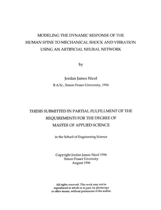
  • 19. In addition, whole body vibration result in a generalized stress response due tn an o w stimulation of the sympathetic nenrous system. This response manifests itself as increases in heart rate, cardiac output, peripheral vasoconstriction, respiratory rate and oxygen uptake. Such stress-induced stimulation of the cardiovascular system may result in fatigue but there are no indications of more serious health effects (Village ef nl., 1995). 2.2.1 Vertebral Effects The spine is a complex structure consisting of a number of rigid elements (vertebrae) connected by flexible, visco-elastic elements (disks). The lateral and posterior views of the spine are shown in Figure 2.1. One such disk and the superior and inferior vertebrae constitute a spinal unit, as pictured in Figure 2.2. BACK AN11 SlUE VIEW OF THE SPINE Figure 2.1 The posterior (left)and lateral(right)views o the human spine. f
  • 20. facet joint branch to facet joinf Figure 2.2 Spinal Unit Exposure to whole body vibration and shock can result in back pain and back disorders. Back pain is a term fox a general class of back ailments which are diagnosed on a subjective basis, whereas (clinical) back disorders are diagnosed through more objective measures (radiological methods, for examplej. There is a high reported incidence of back pain among heavy equipment operators, tractor drivers, truck, bus and car, heavy equipment operators (eg. excavators), and pilots. Paulson (1949) reported that of 23 tractor drivers, 43.5% complained of back pain. Moreover, the study indicated that there was correlation between the reported severity of pain and the roughness of the ground. Among large population of container tractor drivers (540) and truck drivers (633), approximately 40% experienced back pain (Konda et al., 1985; Backrnan, 1983). Beevis and Forshaw (2985) reported an 89% incidence of back pain among trainees for MI13 Armoured Personnel Carriers. Gruber (1976) reported that truck drivers have higher rate o premature deformation of the spinal column, back pain and sprains than f air traffic controllers bus drivers.
  • 21. For incidence of back disorders, Kristen (1981) reported an 81% rate among truck drivers. Similar rates for truck drivers were reported by Schmidt(1969):79.5% versus 61.1% for the control group. Rehrn and Wieth (1984) reported rates of 65% for retired truck drivers, 77% for truck/car drivers, and 80.3% for heavy equipment operators, compared with 62% in the control group. Damage to the spine in response to high amplitude impacts typically consists of end plate fractures, whereas long-term exposure to vibration and/or repeated impacts is usually associated with degenerative damage. This pattern of failure is analogous to engineering materials which can fracture due to a single loading beyond their elastic limit and suffer material fatigue due to repetitive loading. It, therefore, follows that understanding the bio-mechar;lcal properties of the spine will lead to an understanding of its failure mechanisms. A number of researchers have investigated the mechanical properties of the spinal unit in vitro (Crocher and Higgins,l967; Henzel, Mohr, and van Gierke, 1968; Markolf, 1970; and in vivo (Nachemson and Morris, 1964; Christ and Dupuis, 1966; Pope et al. ,1991). Two mechanisms for chronic degeneration of tissues due to long-term exposure of vibration have been proposed: mechanical fatigue and impairment of nutrition. Several studies (Henzel et GI. 1968, Rolander and Blair, 1975; Brinckmann, 1988) have indicated that when the spinal unit is compressed, the disk, being virtually incompressible, bulges only slightly along its radial axes. Thus, any forced displacement of the two vertebrae is due not to compression of the disk but rather an inward deformation of the vertebral end plates. Such findings lead Brinkman (1988) to suggest that disk herniation is a result of repetitive loading of the disk, resulting in a fatigue failure of the disk rather than a single mechanical overload. This argument is supported by clinical symptoms o disk herniation whch include detached pieces of f annular material and sometimes fragments of cartilagenous end plate. Hansom and Mdm (1991) s p e d a t e that tissue damage is partially a result of impaired nutition to the disk and end plate structures. The authors state that vibration may lead
  • 22. to a disruption of blood flow in vessels surrounding the annulus fibrosis and under the endplate, thereby reducing the diffusion of nutrients to tissues. Sandover's (1983) hypothesis links the nutrition and mechanical failure mechanisms. He suggests that compressive loading leads to fatigue-induced micro fractures of the end plate or the subchondral trabecular bone. The repair process leaves deposits of callous which lead to reduced nutrient diffusionto the end plate and the disk, thereby resulting in eventual tissue degeneration. 2.3 Existing Models A number of models have been developed which simulate the response of the human body to vibration and shocks. These models can generally be classified as being either biodynarnic models or physiological models. Biodynamic models attempt to reproduce the dynarnical characteristics of the body, but do not represent real anatomy or neuro- muscular effects. Instead, these models usually contain interconnected springs, masses, and damping elements. Biodynamic models range from lumped parameter models having a single degree of freedom and linear characteristics (Payne, 1991) to discrete parameter models having multiple degrees of freedom1 (Belytschkoand Privitzer, 1978; Amirouche, 1987)and models having nonlinear characteristics (Payne and Band, 1971; Hopkins, 1972). The model parameters were adjusted using measured input and output data to provide the best possible prediction. This undermines the validity of the model (unless it is verified using an independent data set) as it is no longer independent of the experimental data with which it was compared (Arnirouche, 1987). It has been shown A few words about terminology for clarification: The usage of "lumped parameter", "discrete- parameter", and "degrees of freedom" in the literature differs somewhat from conventional engineering usage. In this context. "lumped means the body is treated as several large masses, representing the head: thorax, abdomen. etc., whereas in "discrete" models, the body is represented by individual elements, such as masses for each vertebra. In ;he sybtems theory. both of these models would be considered to be of the lumped parameter type. In reality, most real systems are of the distributed parameter type but to simplify analysis, we lump the system parameters into discrete elements. Funhennore, "the degree of freedom" refers to the system rather than the number of variable model parameters. For ~xarnple, single degree of freedom model of a spinal unit would predict motion (usually a acceleration) in one of the six independent directions of movement available in three dimensions.
  • 23. that the biodynamic response can be predicted reliably within certain ranges of motion using a linear lumped parameter model (Fairley and Griffin ,1989). However, Muksian and Nash (1974) demonstrated that a nonlinear model was required to accurately simulate biodynamic response o17era wide range of frequencies and amplitudes. A separate modelling approach incofporates anatomical structures and their properties as determined experimentally (for example the stiffness and damping of intervertebral discs and ligaments, muscle recruitment patterns and force-velocity characteristics). Passive models of this type representing the geometry and material properties of the vertebral column have been shown to be informative in predicting internal stresses and compression failures (Orne and Lui, 1971; Prasad and King, 1974). Active models incorporating muscle characteristics have been developed for predicting vertebral compression forces in activities such as lifting and carrying (Marras and Sommcrich, 1991; McGill, 1992). These models require a knowledge of body segment kinematics as input data, and for this reason are sometimes referred to as inverse dynamic models. However, these models have not been validated for whole body vibrations and shock environments and, unlike lumped or discrete parameter models, cannot predict body segment accelerations or vertebral compressive forces from a knowledge of vehicle motion (eg. seat acceleration data) alone. 2.4 Standards of Exposure A variety of guidelines exist for the evaluation of human exposure to whole body vibration and shock: International Standards Organization (ISO) 2631 (1985), British Standard 6841 (1987), Air Standardization Coordinating Committee (ASCC) (1982). Of these methods, the most widely used is the IS0 2631, which provides a method for calculating the exposure limit for health effects of vibration. The method of calculation is based on the vector sum of the frequency weighted accelerations at the seat in all three biodynamic axes. The use of root mean square (RMS) acceleration values in the sLmdarDtends to smooth the effect of single, high amplitude events such as impacts or
  • 24. mechanical shocks. For this reason the standard excludes acceleration signals containing crest factors greater than 6. Although crest factors up to 12 are proposed in a draft revision of the standxd, it is widely recogrued that the rms method is inadequate for evaluation of the health effects of non-stationary signals. A more sensitive method of evaluating non-stationary signals containing vibration and shocks is described by Griffin (1986) and is included in Appendix A of the British Standard 6841. This method calculates a vibration dose value (VDV) based on the fourth power of the weighted acceleration signal at the seat, where a,, represents the B 6841 filter output due to acceleration at the seat. (t) S Although the B 6841 does not define limits for health effects, it is estimated that a VDV S of 15 causes severe discomfort, and it is also assumed that increased exposure will be accompanied by increased risk of injury. A revision of t h s standard utilizes a biodynamic model developed by Fairley and Griffin (1989) to weight the accelaration prior to application of the VDV equation. This model, based on the data of 60 subjects exposed to low amplitude vibrations (1.0 ms-2), has a natural frequency at 5 Hz and a critical damping ratio of 0.48. The DRI developed by Payne (1965) and utilized in the ASCC advisory publication is designed specifically for the analysis of the spinal injury risk of large amplitude accelerations (10 to 200 m/s2) in the vertical direction ( +z axis). Unlike the frequency weighting approach of the I S 0 2631 and B 6841, the DM is based on a biodynamic S model having a single degree of freedom. It is assumed that the output of the model, represented by the peak force in the spring component, is proportional to the stress developed in the human body. The model, shown in Figure 2.3, consists of a second order linear system which can be defined by its natural frequency (f,= 8.4 HZ) and
  • 25. critical damping ratio (2 = 0.224). In a draft revision of the DRI, Payne (1991) recommended fn that should be increased to 11.9 Hz with a c of 0.35. m = mass A 112 k = spring stiffness 6 c = damping constant h h = unloaded spring length -C 6 = spring compression 1h (v . ) . y, 1 P I Yc Acceleration input 4477- ground reference Figure 2.3 Biodynamic model used in Dynamic Iiesponse Index. The DRI model acts as a low pass filter, attenuating the higher frequency acceleration components at the seat, and magnifying acceleration waveforms close to the resonant frequency of the model. By focusing on the peak output of the system it avoids the lUvlS "weraging" process contained in the IS0 2631 and more accurately reflects the effect of impacts. Although originally dcsigned to evaluate single impacts, the DRI has been extended to evaluate the injury risk from repeated shocks (Allen, 1976) using a peak stress summation method based on the fatigue failure characteristics of biological materials (Sandover, 1985). In this model the critical DRI for j occurrences of a given acceleration magnitude is expressed as where D q is the DRI value of the acceleration waveform input at the seat, DRI, is the DRI value required to cause injury from a single impact, and ADRI = DRI - I is an offset factor for gravitational loading (Payne, 1991).
  • 26. The ability of the DRI and VDV models to evaluate health effects depends on the degree of accuracy with which their filter outputs simulate th.e human response to vibration and repeated shocks. The response characteristics of the two models upon which these standards are based demonstrate distinct differences as shown in Figure 2.4. In addition, both models describe linear systems, whereas the hurtan response is generally accepted to be nonlinear in nature. The different natural frequencies of the Fairley-Griffin and DRI models representing low amplitude and high amplitude acceleration, respectively, would appear to confirm the nonlinear characteristic of the human body. Furthermore, in vitro compression testing nf !l)mbarl-lumbar2 spinal units have indicated a non-linear foieo-displacement curve( Crocher and Higgins,l967). Thus, it is unlikely that a simple linear model is capable of representing a wide range of vibratio-n and shock amplitudes. 3 . ..-, 2.5 - /I I - I 2 / - I 'z Q) , .& 1.5 - / I 5 . - / I - - - - - - 0.5 - / - ----, 01 . 1oO 10' frequency, Hz Figure 2.4 Magnitude frequency response of the DRI model (dashed line) and the BS 6841 filter (solid line).
  • 27. Artificial neural networks are a class of computational structures which, in some respects, emulate biological neural networks. Some shared characteristics include high connectivity, massive parallelism, and adaptation to stimulus. Artificial neural networks have applications in engineering (modeling, control systems, signal processing, speech recognition), as well as cognitive science and neurophysiology (as models of high and medium level brain function, respectively). They have been used by financial analysts to forecast commodity prices, meteorologists to predict weather, and biologists to interpret nucleotide sequences. A simplified model of a typical biological neuron is shown in Figure 3.1. The neuron consists of three anatomical regions: dendrites, soma, and axon. The dendrites are the receiving terminals for the majority of incoming neural signals. The soma, or cell body, controls the metabolism/reproduction of the neuron, and the axon transmits outgoing signals to other neurons or effector cells such as muscle. dendrites nuclew axon L Figme 32 Biological Neuron. . Neural signals propagate between neurons at connections called synapses. When a neural signal reaches an end terminal of an axon, chemical messengers called
  • 28. neurotransmitters are released from the axon and bind to the membrane of a post- synaptic neuron. Each bound neurotransmitter results i a small change in the n receiving neuron's membrane potential. If, and only if, the net sum of all synaptic inputs causes the neuron's membrane potential to exceed a threshold value, an action potential is produced, and the neural signal propagates to other neurons. A number of factors govern the probability of action potential generation, including the magnitude of excitatory and inhibitory post-synaptic potentials and the effectiveness (or strength) of the synapse. It is believed that long-term modification of synaptic strength - is the basic mechanism through which a biological neural network learns. An artificial neural network (ANN) consists of elementary processing units analogous 'if; bicilogicaf.neurons in function but far less complex. A network of interconnected processing elements (PEs) may be implemented as a computer program or as an electronic circuit. Connections between PEs are unidirectional communication channels with a scalar gain factor called the connection weight. Inputs to each PE are amplified or attenuated by the weight of each connection and then summed. The sum of these weighted inputs is then passed through an activation function, resulting in an output which is distributed to other PEs. Whereas biological neurons fire an action potential only if the the activation threshold is reached, artificial neurons produce an output for all ranges of input signals. The input-output characteristics of the PE depend on the particular activation function chosen. Artificial neural networks adapt through modificabons of the connection weights according to a pre-defined adaptation algorithm, or training rule. The training rule and arrangement of PEs (network architecture) is what distinguishes different types of artificial neural networks. ANN architecture may be classified as either static or dynamic. A static network pefforms a nodnear transformation of the form ):= G(x) wherex E 93" and y E 93" . Static networks are, therefore, memoryless systems since the current output is a function =f mdy the cm-nzntinput- ?%ex n&works are usually referred to as feedforward
  • 29. networks (FFNN)because information flows uni-directionally, from input to output PEs without any cycles. Dynamic networks contain feedback connections and, thus, their output is a function of both the current input and the current network state. Because the output must be calculated recursively, these networks are usually referred to as recurrent neural networks (RNN). In signal processing terminology, recurrent neural networks are equivalent to nonlinear infinite impulse response (IIR) filters. The operation of an ANN can normally be divided into a training phase and a recall phase. During training, input stimulus are presented to the network and synaptic weights are modified according to the training rule. In the recall phase, the adaptation mechanism is normally deactivated and the rietwork simply responds to further stimulii as it has been trained to do. In some cases, as when employed as adaptive equalizers, these two phases can occur at the same time. Training rules may be categorized as being supervised or unsupervised. L supervised n leaming, the network is presented with example input/output data and trained to implement a mapping that matches example data as close as possible. A "supervisor" detects incorrect network responses and adjusts the weights accordingly. The supervisor typically takes the form of a performance criterion, such as the sum of squared errors between the desired response and the network output. Some examples of supervised learning algorithms include Backpropagation (Werbos, 1974; iiummelhart and McLelland, 1986), Cascade Correlation (Hecht-Nielsen, 1987), Learning Vector Quantization (Kohonen e GI., 1988), Red-Time Recurrent Learning (Zipser and f Williams, 1989), and Extended Kalman Filtering (Singhal and Wu, 1989) From the point of view of pattern recognition, supervised leaming utilizes pattern class membership information (Kosko, 1992). If the network performs a nonlinear mapping o the form y = G(x)wherex E 9In and y E *;Xm, then the training process partitions the f input space 32" into k pattern classes of dimension M. After training, the network mput h&r"a*e degree t which the input pattern be1ongs to a particular pattern the o
  • 30. class. Since the membership classes are known a priori, the supervisor can detect incorrect pattern classifications during training and correct them through weight adjustments. In unsupervised learning, the pattern membership classes are not known beforehand. Rather the network is presented with unlabelled patterns and evolves its own membership classes, or pattern clusters. Patterns are clustered on the basis of similarity defined by some metric, such as the Nearest Neighbor Rule (Simpson, 1993). Due to this behavior, such neural networks are described as self-organizing. Some examples include Kohonen Self-organizing Map (Kohonen, 1984),Adaptive Resonance Theory (Carpenter and Grossberg, 1987), Discrete Hopfield Networks (Hopfield, 1982),and Temporal Associative Memory (K ..,KO, 1988) 3.1 The Multi-Layer Perceptron Probably the most commonly used ANN is the multilayer perceptron (MLP), also referred to as a multilayer feedforward network . These networks are modification ~f the single layer, linear Perceptron that was first developed by Rosenblatt in 1958. The structure of a MLP consists of a number of PEs, arranged in layers as depicted in Figure 3.2. Information flows from the input layer to the output layer without any feedback.
  • 31. input layer Figure 3.2 Multilayer Perceptron PEs in the input layer are typically data buffers which distribute the input to the rest of the network. PEs in the hidden layer typically consist of a summer and an activation function. Each input to the summer is multiplied by the connection weight. The activation function introduces a non linearity which makes these networks powerful modeling tools. Without it, the network can at most perform a linear mapping. Output PEs may ha.ve nonlinear or linear activation functions, depending on the application. Consider a MLP consisting of M layers. The i'th PE in the l'th layer (Figure 3.3) produces an output that is a nonlinear function of weighted inputs from PEs in the previous layer. The inputs are first summed and then passed through an activation function F(m). The input to the activation function is given by "-1 wbxj ( t )+ b: I /-I v,!( t )= where n,-, is the number of PEs in the (I-1)'th(or previous) layer, w; is the weight connecting the j'th PE in layer I-1 to the i'th PE in layer I, xi-' ( t ) is the output of the j'th PE in the (I-1)'th layer, and b: is the threshold parameter, or bias, associated with the I'th layer.
  • 32. Figure 3.3 Basic Processing Element. The PE output is then given by xi!( t ) = F [ V ; ( t ) ]. (3.2) Using the above equations the entire network (Figure 3.4) can be described by "1-1 x ( t )= F [ X W : j=1 1 1-1 ~ X ,( t ) + b:] for I = 1,...,M (3.3) layer I = 0 layer I = 1 layer 1 = 2 Figure 3.4 M layer Perceptron
  • 33. The number of inputs and outputs then becomes, respectively, 11, and PI,,, . To differentiatethe network input from the input to any PE, we can redefine the input to the j'th PE of the input layer (1=0) as 14, ( t )= x ( t ) ; (3.4) Similarly, to differentiate the network output from the output of any PE, we can redefine the ouput of the i'th PE of the output layer (l=M) as ji( t )= xy ( I ) where F i ( t )is the network approximation of the target variable y, ( t ) . The most common choice of activation function are either the sigmoid or the hyperbolic tangent but, in theory, any differentiable function can be used. The sigmoidal activation function is described by whereas v is the sum of weighted inputs to the PE. Similarly, the hyperbolic tangent function is defined by An advantage of these two functions is that their respective first derivatives can be expressed as a simple function of itself. For example, the first derivative of the sigmoidal function is given by
  • 34. 3.2 Training During training, the network is presented with example inputs and outputs. The weights and bias values are then adjusted to minimize some cost function, typically the sum of squared errors between the network output and the actual output. To elaborate on this concept first let us define a three layer network (M=2) with a single PE in the output layer. The total number of network parameters (weights and biases) is then N, + + 1. Now define a network parameter vector, 0, that contains both the = n, (no 2) weight and bias values, such that T 0 =[e, ... e,] . Furthermore, let The cost function used in training the network is then The objective of training is to find the value of 0 for which ~ ( O ) iminimized. The s optimal vector is found iteratively using the generalized update equation where s is the search direction on the error surface at iteration step k, and a is a small positive constant called the leaning rate which determines the adaptation step size.
  • 35. 3.3 Steepest Descent Algorithms The simplest search direcnon is called steepest descent, in which the parameter change is along the negative gradient of the error surface J. That is, we choose where Define the gradient of the network output with respect to O as Then it can be shown that Equation 3.13 can be expressed as The update equadon then becomes The most popular form of steepest descent for neural networks is the backpropagation algorithm first proposed by Werbos (1974) and modified by Rummelhart and McLelland (1986). Backprogation takes its name from how the weight changes are ordered. Updates are made from the output layer to the input layer, using calculation of the error dependent on the earlier steps, so that the error tends to propagate backwards through the network. The main disadvantage of backpropagation and steepest descent
  • 36. in general is that the algorithm may converge to a local minimum of the error function. In addition, convergence tends to be slow due to the typical shape of the error surface. Sigmoidal activation functions tend to result in error surfaces w-hich alternate between very flat regions, in which learning is painstakingly slow, and steep regions which can causes the algorithm to become unsiable (Hush and Horne, 1993). 3.4 Gauss Newton Methods A more efficient search direction is used in Gauss-Newton-based methods such as Levenberg-Marquardt (Marquardt, 1963), Extended Kalman Filter, and Recursive Prediction Error (Chen, Billings, and Grant, 1989). These algorithms use second order derivative information of the error surface which results in an increased rate of convergence. Unfortunately they also require significantly more computation, and unlike backpropagation do not take advantage of the parallel structure of the network. Gauss-Newton methods modify the steepest descent search direction through multiplication of the negative gradient by a special matrix which contains information about the error surface shape. This matrix is the inverse of the approximate Hessian of the cost function. The appro::imation of the Hessian is 1 " H(O)=-CY(t,O)YT(t,0)+hl for h > 0 N ,=I (The addition of the second term ensures that H(O) is nonsingular.) The modifued search direction then becomes 3 5 Generalization. .
  • 37. Generalization is the ability of the trained network to perform well on unseen dat,~ sets. Cross validation is the most common test for generalization. Prior to training, a subset of the available data called the testing set, is set aside for validation purposes. This set is assumed to be contained within the input space bounded by the training datcl. In other words, it should represent data that is similar, though not identical, to that used for training, where the definition of similar is application specific. The trained network's performance on the testing set indicates the degree to which the n~odcl represents the underlying system as opposed to merely being a good fit to the training data. Network generalization is affected by the number of data samples in the training set (and how well they represent the problem), the complexity of the underlying systcm, and the complexity of the neural network model (Hush and Horne, 1993). In general, as the amount of training data increases, so too will the ability of the network to generalize. The complexity of the neural network is measured by the number of hidden layer I'Es and the number of hidden layers. These parameters determine the complexity of the nonlinear function that can be approximated. If too few PEs are present, the representational capacity of the network will be limited. On the other hand, if there are too many, the network will be prone to overfitting the training data. Optimal performance will be obtained when the complexity of the neural network matches that of the system or function to be modeled. The number of hidden layer PEs can be optimized using cross validation. A plot of the performance function over the testing set will often show a minimum value when the structure of the neural network corresponds to the trre system structure (Billings, Jamaluddin and Chen, 1991). A similar strategy is to compare the performance of the network on the training set and the test set. The optimal number is obtained when the prediction error is approximately the same on both sets. Some strategies, such as the Cascade Correlation method, add PEs during training as needed.
  • 38. The number of hidden layers is similarly related to network's representational ability. Increasing the number of hidden layers results in an increase in the dimensionality of the problem space, making it easier for the network to approximate the nonlinear function. It has been shown that a single hidden layer is sufficient to approximate any continuous nonlinear function (Funahashi, 1989; Cybenko, 1989). Therefore, this same increase can be achieved by adding PEs to a single hidden layer but the number required may be astronomical. An analogous situation occurs in digital circuit design in which any binary function may be implemented as a sum of products (or product of sums) but may require a large number of logic gates. The total number of logic gates may be drastically reduced by instead using several layers of logic. Various other strateges exist to increase network generalization: early stopping, pruning and complexity regularization. Early stopping (Cohn, 1993)involves limiting the number of training iterations. During the learning process, the performance of the network on the training set will continue to improve. However, at some point the performance on the testing set will decrease. Overtraining causes the network to learn the particular noise realization of the training set, as opposed to learning the input- output behavior of the underyling system. Network pruning is based on the view of training as a process of encoding system information in the network weights. It assumes that a trained network contains redundant information which may be removed, thereby decreasing the network complexity. Pruning strategies usually start with a large network and systematically delete weights and PEs. One approach is to simply delete connections with very small weight values. It has been shown that a more effective strategy called Optimal Brain Damage (Cun, Denker, and Solla, 1989) is to delete the weights with the smallest salimnf, i.e. whose removal disturb the solution the least. Complexity regularization (Larsen and Hanson, 1994)increase generalization by penalizing netwmk solutions that are overly complex. The penalty is imposed by adding a complexity term, such as the sum of squared weights to the cost function. This penalty term causes the weights to converge to smaller absolute values than they
  • 39. otherwise would. A common method of regularization is through weight decay in which the cost function takes the form In this equation, N represents the number of training patterns, 0; is the i'th welght contained in the vector 0, and h is the weight decay parametsr which controls the - . influence of the second term relative to the squared error term. Weight decay results in a smaller average weight size which tends to discourage overfitting.
  • 40. CHAPTERRECURRENT 4 NEURAL NETWORKS FOR SYSTEM IDENTIFICATION Two fundamental approaches exist for developing a mathematical model of a system. In the analytical approach, physical laws such as the conservation of energy or mass are used to develop differential or difference equations. Analytical modeling may be used only when adequate knowledge about the system is available and when the system is not overly complex. When these conditions do not hold, an alternative strategy is identify the system from input and output observations. System identification is one of the main concerns in the discipline of mathematical systems theory. Over the past five decades, considerable mathematical tools have been developed for analyzing and designing systems. Most of these tools are based on linear algebra, complex variable theory, and the theory of ordinary, linear differential equations (Narendra and Parthasarathy, 1990). As a result, there exist well-developed techniques for the analysis of linear systems. A similar set of tools does not exist for nonlinear systems and, consequently, modeling such systems is considerably more difficult. The purpose of this chapter is to introduce some fundamental concepts of system identification, and to discuss recurrent neural networks in the context of nonlinear systems identification. 4.1 System Identification: Preliminary Concepts What is a system? Sinha and Kuszta (1983) define a system as "a collection of objects arranged in ordered form, which, in some sense, are purpose or goal directed." More specifically, a system transforms a set of inputs, or causes, into a set of outputs, or
  • 41. effects. The form of the inputs, outputs, and the type of transformation distinguishes one system from another. Systems may be categorized as being either static or dynamical. A static system is memoryless in that its output is a function of the current input only. In contrast, a dynamical system generates an output that is a function of the input as well as the current state of the system. Since the current state is determined by past states and previous inputs, a dynamical system has memory. In addition, systems may be characterized on the basis of stability, causa:ity, linearity, luxnpedness, and time- invariance. For additional discussion of these topics, the reader is referred to any introductory textbook on systems theory such as Chen (1989)or Oppenheim and Schaffer (1989). The model of a system may be mathematically defined by an operator, P, which maps the input space U into the output space Y. P may be realized in a variety of mathematical forms, such as differential equations, difference equations, or as a transfer function. For static systems, U and Y are subsets of %" and %", respectively. For dynamical systems, U and Y are subsets of bounded integrable functions defined on the intervals [0, T] or [Of-) (Narendra and Parathasarathy, 1990). The goal of system identification, then, is to determine an operator which approximates P according to some criterion. Figure 4.1 depicts a single-input, single-output (SISO) system to be modeled, where u(t) is the input signal, w(t) is additive system noise, r(t) is the unobservable system output, n(t) is measurement noise, and y(t) is the observable system output. Given a set of measured input data, u(t), and output data, y(t), the objective is to determine P such that
  • 42. for some E > 0 and some defined norm, denoted by ji*/), such as the root mean squared ~ I Z error. j ~ ~ w(t> Figure 41 System identification approach. . In other words, the system is identified by assuming a parametric model of some suitable structure and then adjusting the parameters such that the discrepancy between the model output and the system output is minimized. The model accuracy will depend on a number of factors such as the choice of model structure, the parameter estimation method, the type of input signd, the complexiw of the system, and the nature of the disturbances, w(t) and n!t)- System identification approaches may be "on-line"or "off-line". When the model is constructed off-line, input and output data are recorded and stored in computer memory. The model is then constructed in batch mode, meaning all at once. The advantages of off-line methods are a greater choice of estimation algorithm and a greater freedom in selection of input signals. For these two reasons, the estimation accuracy of these methods are typically superior to on-line approaches. With on-he system idefitificatioii, mode! parameteis are updated remsively at each sampling instant. Such methods are suitable for modeling a system whose characteristics change with time, or when it is not practical to wait for a l the data to be l solfected. An example application is an adaptive equalizer which corrects distortion in channels. r4d-antages of the on-line approach are that a l the data need comunica~on l
  • 43. not Se stored and special input is not required. However, since computation of parameter adjustments must be a fraction of the sampling period, the choice of estimation algorithms is limited. 411 Input-Output Models .. When identifying a system based on input-output data, a common approach is to express the system as function of delayed inputs and outputs. This formulation of the modeling problem may take one of two forms: the series-parallel model or the parallei model. In the series-parallel model, the predicted output, j ( ~ is expressed as a function ) of previous in puts,^, and previous measured outputs,y, as expressed by where m and I are the orders of the input-output model, respectively; and P is the model operator ( a linear or nonlinear function). This model is appropriate for applications in which a one step-prediction is required. In other words, the model is intended for use on-line (when the system's output is available in real-time). In some applications the model is required to be used off-line, i.e., when the system's output is not easily obtained in real-time. I this case, the parallel model must be used n in which the actual lagged outputs in Equation 4.2 are replaced by lagged values o the f model's predicted output. Thus, the parallel model is expressed as The disadvantage of the parallel model is that convergence of the model parameters to the desired values is not guaranteed. Even for the linear case, stable adaptive laws for the parallel modd have yet to be found (Narendra and Parathasarathy, 1990). On the other hand, if the system i 5o~ded-inpat/bomded-output s stable, the series-parallel
  • 44. model is guaranteed to converge (Narendra and Parathasarathy, 1990). Moreover, if the output error drops to a small value such that ? ( t ) approximates y ( t ) , then the series/parallel model may be replaced by the parallel model. That is, once the parzmeters have been established, the seriesi'parallel model may be operated off-line by feeding back its own predictions in lieu of the system outputs. 4.1.2 Model Order The performance of an input-output model not only depends on the method of function approximation, but also on the determination of the correct model orders (He and Asada, 1993). In general, the order of a model is the number of state variables required to adequately characterize the dynamics of the system. For continuous-time models, this quantity is equivalent to the degree of the system's characteristic equation or the order of the describing differential equation. For discrete-time models, the model order refers to the number of lagged inputs and outputs in the series-parallel or parallel models. Failure to include adequate dynamics in the input-output model will likely lead to a poor model fit to the data (Billings et aI., 1991). Therefore, it follows that a trial-and- error approach may be taken to determine the required number of lagged inputs and outputs. Specifically, the prediction error will show a minimum for those lag values which are optimal. However, this approach results in excessive computation especially when other model parameters must be optimized. In other words, if the model orders can be determined lz priori, then optimization of other parameters is more efficient in terms of time and computations. N u m e r ~ u such methods have been developed to identify the correct model orders for s linear systems (Woodside, 1971; Wellstead,. 1976; 1978; Young et al., 1980). However, few results have been reported for nonlinear systems. One recent method (He and Asada, 1993) exploits the continuity property of nonlinear functions which represent input-output models of the system. This techruque requires only measured input-
  • 45. output data and has been shown to be effective for determining the correct lags for chaotic dynamic systems and non linear plant models. 4.1.3 The Effects of Noise Measurement data is inevitably contaminated with noise, from estermi a i d internal sources as well as from the measuring instruments themselves. When iderdifying a system based on input and output observations, noise can result in a biased estimation of the true model parameters. Bias is a statistical term which describes how close the average estimate is to the actual value of the parameter. For example, the parameter estimate, 6, is said to be unbiased if and only if where E{*) is the expectation operator. In other words, the average value of a set of estimates will, in fact, be the true value. A biased model will likely predict well for the set of data on which the model was trained, but relatively poorly on an unseen data set. That is, the model is biased towards the training set data. This discrepancy indicates that the model provides a curve fit to the data but does not represent the underlying system. Thus, bias is closely related to the concept of generalization. A common strategy to remove bias is to model the noise process. For example, if the system is perturbed by additive, coloured noise, a linear filter can be identified to remove this effect. When the system is linear, a noise source applied anywhere in the system may be transposed to the output (using the principle of superpositionj and dealt: with in this manner. For nonlinear systems, superposition does not hold and other methods must be applied.
  • 46. One strategy is to choose a nonlinear model structure based on assumptions of the noise source location. Depending on where the disturbance is applied three variations of input/output models may be applied. In the output error model (Equation 4.5), it is assumed that the disturbance is applied at the output, but does not feed back into the system and, therefore, does not effect future outputs. This assumption is generally true when the major source of noise is on the output measuring device. r(t) = P[u(t - I), ...,u(t - l ) ,r(t - 1),...,r(t - m)] = Y(Q r(tj -t where u(t), r(t), n(t) ,and y(t) are defined as in Figure 4.1 above. This assumption leads to the predictor which is equivalent to the parallel model of Equation 4.3. In the NARX (Nonlinear Auto-Regressive with Exogenous inputs) or equation error model, the disturbance is also applied to the output of the system but in such a way that it feeds back and affects future outputs. This system is described by the following equations: r(t) = P[LL(~ ...,u(t - I ) , r(t - l), ...,r(t - m)] + n(t) - I), y(t>= r(t) This system results in the predictor m= h ( t - I), ..-, - l ) ,y(t - I), .*. u(t ,y(t - m)] which is equivalent to the series-parallel m d e l of Equation 4.2.
  • 47. Finally, with the NARMAX (Nonlinear Auto-Regressive Moving Average with Exogenous inputs) model, it is assumed that the noise is applied to the input of the system, such that the output is a function of the current and previous noise samples as described by r(t) = P[u(t - I),. ..,u(i - 11,r(t - I), ...,r(t - in), w(t - w(t - p ) ] -tn ( t ) (4.9) YO)= r(t> where w(t) is the system disturbance. In this case, the predictor is described by where e(t) = y(t) - Z,(t). The notion of feeding back the residuals (the e(t)'s ) is based on a principle of estimation theory that states the optimal estimates occur when the residuals are uncorrelated with all combinations of past inputs and outputs. That is, as the prediction improves, e(t) increasingly resembles white noise. 414 Choice of Input Signals .. Correct identification of a system also requires the use of an appropriate input signal. The input should be such that it excites all modes of the system (Sinha and Kuszta, 1983). For linear systems it is sufficient that the input has a flat power spectrum over the frequency range of interest, so that the system is excited by a wide spectrum of frequencies. Ideally, the best choice is an impulse function, but such signals are impossible to generate in practice. A suitable alternative is a white noise signal such as the pseudo random binary sequence (PRBS).
  • 48. For nonlinear systems, the PRBS is not necessarily adequate to excite all the modes because, although its spectruin is flat, it has a constant amplitude in the time domain. In linear systems a constant amplitude can be used since the response at any other amplitude will only differ in amplitude (i.e. by a scaling factor) but not in frequency. This scalability of response does not h d d for nonlinear systems, which may exhibit completely different responses for two signals of similar shape but unequal amplitudes. Intuitively, then the PRBS may be modified for nonlinear systems by allowing it to vary in amplitude. 4.2 Modeling Dynamical Systems with Recurrent Neural Networks Linear system identification techniques are well-known and numerous: frequency response method, step response method, deconvolution, correlation method, least squares estimation, Kalman filtering, maximum likelihood, and instrumental variables. These methods benefit from the well-developed theory of linear systems and the simplificationswhich come with the assumption of linearity. For example, it is well- known that a linear system is stable if the roots of the characteristic equation are inside the unit circle. However, for nonlinear syste~ts, equivalent condition exists and no stability must be cheeked on a system-by-system basis (Narendra and Parathasarathy, 1990). Furthermore, if the order of a linear system is known then the m d e l stmcture is uniquely defined and system identification reduces to the problem of parameter estimation. In contrast, nonlinear systems have an infinite variety of possible representations for a given set of input output observations (He and Asada, 1993). Thus, the choice of model structures must be chosen from a specified set of model classes which are assumed to have the ability to realize the system's input-output behavior (Levin and NarendraI1996). In other words, the type of model must be justified for the intended application. %me early methods for modeling nonlinear systems include the works of Voltena ff 9 9 ,the H m - 51 m d d (Chang and Lurrs, 1971) and nonlinear least squares
  • 49. estimation (Hsia, 1968). More recently, numerous nonlinear function approximation and modeling approaches have been developed: radial basis functions (Powell, 1987; Moody and Darken, 1989), Nonlinear Auto-Regressive Moving Average with exogenous inputs {NARMAX)models (Leontardisand Billings, 1985), fuzzy logic (Takagi and Sugeno, 1985), local technique (Farmer and Sidorowich, 1988). Artificial neural networks, in particular, have received considerable attention for modeling nonlinear dynamical systems ( Narendra and Parathasarathy, 1990; Chen ef nl., 1990; MacMurray and Kimmelblau, 1993; Minderman and McAvoy, 1993; Fernandez ef al., 1993; Kechriotis et al., 1994; Puskorius and Feldkamp, 1994). Numerous classes of artificial neural networks can be used to model a dynarnical system, including radial basis function networks, recurrent neural networks, and multi- layer perceptrons. To date most applications have focused on the latter due to the availability and simplicity of effective training algorithms such as backpropagation. A common approach is the time-delayed neural network which can be implemented using a multi-layer perceptron in which the input layer consists of a tapped delay line of inputs (Figure 4.2). However, since the model memory is determined solely by the number of input PEs, this approach is limited to systems of relatively low order. Figure 4.2 Time-delayed neural network.
  • 50. A variation of the time-delayed neural networks is to also include delayed system outputs in the input layer, resulting in the NARX model of Equation 4.7. While there is an appearance of recurrence in the NARX case, the network is actually static because the lagged outputs consist of actual system measurements. We now turn our attention to the case of truly recurrent neural networks. Recurrent neural networks, introduced in the works of Hopfield (1982), have long been recognized for their powerful mapping and representational capabilities. Because a RNN has feedback, its memory capacity exceeds that of a time-delayed neural network even when a fraction of the number of PEs are used. (Using signal processing terminology, a time-delayed neural network is a nonlinear finite impulse response filter whereas a RNN is a nofinear infinite impulse response filter) Despite this advantage, only in recent years have their use become more popular due to the advent of effective 2nd order training algorithms (.e.g. Real-time recurrent learning ,Extended Kalman Filtering, Recursive Prediction Error.) A number of different archtectures have been developed including Hopfield networks (1982), recurrent multi-layer perceptrons ( Fernandez et al., 1990) ,and Elman networks. These variations fall into one of three categories: externally-recurrent, internally recurrent, and fully-recurrent. In an externally-recurrent network (Figure 4.3), information from the output layer feeds back to PEs in the input layer. A network may also be internally-recurrent (Figure 4.4), in which information from one layer may feed back to itself or other layers. The most general case is the fully-recurrent network (Figure 4.5) in which all PEs are interconnected.
  • 51. Figure 4.3 Externally-recurrent neural network. Figure 4.4 Internally-recurrent neural network.
  • 52. wll Figure 4.5 Fully-recurrent neural network. The internally- and fully-recurrent versions have the advantage that the exact number of lagged inputs and outputs does not have to be determined a priori (MacMurray and Himmelblau, 1993). Rather, these networks have their own internal memory which stores information about the past. On the other hand, these networks require more computationally-expensivetraining algorithms due to their inherently recursive compared with structures. (Real-time recurrent learning has a complexity of 0(w2) O ( w ) for standard backpropagation, where w is the number of adjustable .veights). Moreover, an externally-recurrent network can be trained using actual system outputs in the input layer as opposed to the network's own predictions. In other words, the network is trained as a series-parallel model, which facilitates parameter convergence, and then operated as a parallel model, whereby the network's predicted outputs are fed back to the input layer.
  • 53. 5.2 Statement of Problem Simply stated, the objective of this thesis is to model the mechanical response of the spine to seat-imposed vibration and shocks. A system identification approach has been taken to meet this objective, so that the model will be developed using experimentally measured input and output data. Furthermore, since evidence exists to suggest that the mechanical response is nonlinear in nature, a nonlinear systems identification approach will be taken which will utilize an artificial neural network. The problem is described by the system in Figure 5.1 (a). The input to the system, s(t), is acceleration at the vehicle seat, and the output, v(t) is acceleration at the vertebrae. The seat motion consists of linear and angular acceleration in six degrees of freedom as depicted in Figure 5.1 (b). (the x,y, z axes and rotation about these axes). Seat acceleration transmits upwards through the spine resulting in acceleration of each vertebra, also in six degrees of freedom. Moreover, the response of the spine will differ at each vertebra. ~(t) human body + ~(t) Figure 5.1 (a) Block diagram of the seat-spine system; (b) Degrees of freedom in terms of acceleration of the human body.
  • 54. The system in Figure 5.1 (a) can be described mathematically by an operator, P, which maps the seat acceleration to the vertebrae acceleration such that where and Note that v(t) is matrix of dimension N x 6 matrix where and N is the number of vertebrae in the spine. Thus, P maps the six acceleration components at the seat to the six acceleration components at each of the N vertebra. To simplify the modeling task, a number of constraints are imposed. Firstly, the problem is limited to seat and spine acceleration along the z-axis. One disadvantage of this approach is that it ignores the cross-axis transmission; an impact at the seat in the x or y axis will result in acceleration in the z-axis at the vertebral level. However, this constraint may be justified on several grounds. Shocks in the z-axis typically have the largest amplitude since mechanical impacts travel upwards through the vehicle and seat into the body, and therefore presumably have the greatest effect on tissues. As some studies suggest compression of the spine, due largely to z-axis shocks, results in fatigue failure of vertebral end plates. Secondly, the model will only predict acceleration at a single vertebra. This constraint greatly reduces the complexity of the model and the number of computations required
  • 55. in the identification process. It should be fairly straightforward to extend the model to other spinal levels. The !=mbar level was chosen because the main health effect of exposure to vibration and mechanical shock reported in the literature is l o w ~ r - b ~ ~ c k pain. Moreover, while only the response at a single lumbar vertebra has been modcled, it has been shown (Cameron et nl., 1996) that the shape and magnitude of the rtlspnnst at adjacent vertebrae is similar. The third constraint is optimizing the model based on data collected for only one subject. Ideally, the model would be universal such that it predicts the response for tht* entire population of vehicle occupants. Realistically, we can only hope to characterize the average response. System identification techniques are intended for modeling one particular system, whether it is a biological process or an industrial plant. In this case, however, we wish also to characterize an entire class of systems &r.snore than one subject) so that the resulting model is universal in its applicability. A universal mode will not only depend on how well we identify this one system but also on the degree o f variance between individuals and the degree to which the chosen subject represents the average response Given the above constraints, the identification problem is now formulated as follows: We wish to predict the z-axis acceleration at the fourth lumbar vertebra (L4) for one particular subject of a military population, for the types of z-axis seat i n w x i s and vibration experienced by occupants in tactical ground vehicles. The developed model is intended to predict the spinal response based on vehicle seat only, as it is impractical to measure the vertebral acceleration of vehicle passengers in the field. The simplified system to be identified is shown in Figure 5.2 human body Figure 52 Simplified seat-spine system, showing the seat z-axis acceleration, s,(tj, and the z-axis . acceleration at the fourth lumbar vertebra, vZrL4(t).
  • 56. if the model can predict the lumbar acceleration then methods exist to relate this to effective stress on the vertebral tissues. Using material fatigue theory and epidemiological data of back injuries i t is possible to estimate the probability of injury due to exposure to mechanical shocks IBC Research Incorporated, 1996). The exposure time for vehicle occupants may then be limited to maintain the risk of injury below an acceptable level. The strategy to be employed in the dtvelopmen t of the model is as follows: i i j; Experiment Choose Model ! j Validate Model Figure 5.3 System Identification Flowchart.
  • 57. The flowchart illustrates the iterative nature of system identification. In many cases it n a y be necessary to back up a step and re-examine the assumptions made about the system. Most development time is spent in steps 3 to 5. We try to adjust the structure and estimate parameters to obtain a good model. If we are unsuccessful we may haw to take more drastic measure such as re-designing the experiment (perhaps the test data does not excite all the system modes adequately) or choosing another class of model. These steps are discussed in the following sections. Except where noted, the data processing and model development was performed using the MatLab software package (Mathworks),running on an IBM 486 - 50 MHz Personcd Computer. The neural network training and simulation routines were provided by a publicly available neural network MatLab toolbox (Norgaard, 1995). In many cases, these programs were modified to suit this application. All MatLab m-file scripts are provided in Appendix A. 5.2 Selection of model class 5.2.1 Justification for a nonlinear model The choice of a nonlinear model was based on several pieces of evidence which indicate that the response of the spine to seat shocks is nonlinear. Cameron et nl. (1996) found that a nonlinear relationship exists between the peak z-axis acceleration measured at L4 and the peak z-axis seat accleration in response to positive and negative seat shocks. This relationship is illustrated ir.Figures 5.4 and 5.5. If the response was linear then one would expect the plotted ratios to be constant over different ranges of seat shock amplitudes, based on the homogeneity property of linear systems (Chen, 1989).
  • 58. Figure 5.4 Peak transmission ratio versus frequency for positive amplitude seat shocks. (From Cameron ef al., 1996). Figure 5.5 Peak transmission ratio versus frequency for negative amplitude seat shocks. (From Cameron ef al., 1996). In addition, the shape of the response at the spine changes with the amplitude of the seat shock. This is demonstrated in Figures 5.6 and 5.7 which show the L4 acceleration in response to 4Hz shocks of amplitudes 3g and -3g, respectively. If the response was linear then the two responses would have the same shape and differ only by a scale fac'x of -1.
  • 59. 1.9 2 2.1 2.2 2.3 time (s) Figure 5.6 L4 response (dashed line) to 3g, 4Hz seat shock (solid line). time ( s ) Figure 5.7 L4 response (dashed line) to -3g, 4Hz seat shock (solid line). The nonlinear response of the spine has also been reported by several researchers (Crocher and Higgins, 1967; Griffin, 1986). Finally, the different natural frequencies of the Fairley-Griffin and DRI models representing low amplitude and high amplitude vibration, respectively, imply the nonlinear characteristic of the human body. Hence, the use of a nonlinear model appears to be warranted.
  • 60. 5.2.2 justification of the neural network model The choice of an artificiaI neural network to model the system is justified on the basis of the Stone-Weierstrass theorem (Cotter, 1992)which states that any continuous function can be approximated arbitrarily closely by a polynomial of sufficient degree.. Stone- Since it has been demonstrated that a neural network with an arbitrary number of PEs in a single hidden layer is capable of approximating any polynomial (Cybenko, 1989; Funahashi, 1989), it follows that an ANN is a universal approximator. A corollary to this axiom is that a recurrent network of correct order can model any continuous system. To model the system, an externally-recurrent neural network was chosen which represent the parallel identification model ( t )= [ ( t- 1 ) ..( t - 1 ) ( - 1 ) .. ( t - m)] This above mcdel is the nonlinear output error(N0E) formulation given in Section 4.2 and is recurrent of order m. The choice of this model class, as opposed to the NARMAX, or NARX formulation, was based on the need for the model to be used off- line. (Recall that both the N A R U X and NARX models require the actual system output to generate their prediction.) It is possible to first train the model using the NARX structure and then to use this model off-line. Training involves the finding the set of network parameters for which Equation 3.11 is minimized. W e n Equation 4.2 (the NARX model) is substituted into the above equation for?(t), the minimization process is identical to the maximum likelihood estimation approach (Werbos, McAvoy, and Su, 1992). We will, therefore, refer to the network parameters optimized in this manner as the maximum likelihood values. There are two problems with the NARX (or maximum likelihood) approach. Firstly, the resulting model is optimized for single-step ahead prediction and likely will not perform well as a multistep predictor. During multi-step forecasting, prediction errors