

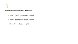

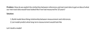
![A a i g Wi d Da a
Le ' ad da a f a e a a d chec !
I [1]:
O e a da a h d eed / a 30, 45, a d 58 he gh , e e a e C, a d d d ec
, 10- e e a .
(The e da a a e a a ca a d I ge e a ed he .)h eb
O [1]: d_30 d_45 d_58 di
i e
1999-12-31 16:00:00 3.39 3.73 3.84 12.37 243.68
1999-12-31 16:10:00 3.27 3.65 3.81 12.22 250.02
1999-12-31 16:20:00 3.31 3.63 3.80 12.12 252.29
1999-12-31 16:30:00 3.78 4.26 4.38 12.04 249.54
1999-12-31 16:40:00 3.96 4.38 4.52 11.99 254.50
impor a da as d
da a = d. ad_ a ('./da a/ _ a . a ')
da a. d(2). ad()](https://image.slidesharecdn.com/predictingthewind-datascienceinwindresurceassessment-florianroscheck-201122042944/85/Predicting-the-Wind-Data-Science-in-Wind-Resource-Assessment-10-320.jpg)
![Le ' ge a feel f he i d da a b l i g he !
In [3]:
... , ha l k e e !
O t[3]:
# Pl i d eed ime e ie
impor bright ind as b
anemometers = ['spd_30','spd_45', 'spd_58']
b .plot_timeseries(data[anemometers])](https://image.slidesharecdn.com/predictingthewind-datascienceinwindresurceassessment-florianroscheck-201122042944/85/Predicting-the-Wind-Data-Science-in-Wind-Resource-Assessment-11-320.jpg)
![Le ' a i g e da ee e de ai !
In [4]:
Ob e a i : Wi d eed a ie a h gh he da . Highe heigh ea highe i d eed.
O [4]:
b .plo _ imeseries(da a.loc['2019-03-11',anemome ers])](https://image.slidesharecdn.com/predictingthewind-datascienceinwindresurceassessment-florianroscheck-201122042944/85/Predicting-the-Wind-Data-Science-in-Wind-Resource-Assessment-12-320.jpg)
![Which di ec i n d e he ind c me f m? Le ' l a f e enc e !
I [5]:
O [5]:
. _ a ( a a[' _30'], a a[' '])](https://image.slidesharecdn.com/predictingthewind-datascienceinwindresurceassessment-florianroscheck-201122042944/85/Predicting-the-Wind-Data-Science-in-Wind-Resource-Assessment-13-320.jpg)
![Le ' ad c i a e de ( ) a d ai a i da a!ERA5
I [6]:
C i a e de ica d i d eed a g d e e a d ha e 1-h e i .
( h h I d aded ERA5 da a a d h h I d aded ai
a i da a.)
Thi eb hi eb
O [6]: pd di mp
ime
1999-12-31 16:00:00 4.548827 249.010856 12.370013
1999-12-31 17:00:00 3.981960 251.738388 11.915547
1999-12-31 18:00:00 2.607753 249.791620 11.245783
1999-12-31 19:00:00 1.559933 233.880179 9.782310
1999-12-31 20:00:00 1.359054 231.334928 10.454369
f om a b impo Pa
impo a da a d
_da a = ' a5_0': ' a5_0. a ',
' a5_1': ' a5_1. a ',
'MYF': 'MYF_200001010000_202003070000. a ',
'NKX': 'NKX_200001010000_202003070000. a ',
'SAN': 'SAN_200001010000_202003070000. a '
fo a , in _da a. ():
_da a[ a ] = d. ad_ a (Pa ('./da a/'). a ( ))
_da a[' a5_0']. ad()](https://image.slidesharecdn.com/predictingthewind-datascienceinwindresurceassessment-florianroscheck-201122042944/85/Predicting-the-Wind-Data-Science-in-Wind-Resource-Assessment-18-320.jpg)
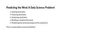
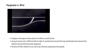
![Le ' plo me ma ind peed da a again he da a from he ERA5 clima e model!
I [7]:
Good ne : De pi e being ph icall far a a , here eem o be grea imilari ie be een he clima e model
and he me ma da a. (Thi i no al a he ca e, b i i here o make hi orial f n and ea .)
O [7]:
l _da a = d.c ca ([da a[' d_58']. e am le('1W').mea (), l _da a['e a5_0'][' d']. e am le('1W').mea ()], a i =1)
l _da a.c l m = ['Mea eme ', 'LT Refe e ce']
b . l _ ime e ie ( l _da a, da e_f m='2017')](https://image.slidesharecdn.com/predictingthewind-datascienceinwindresurceassessment-florianroscheck-201122042944/85/Predicting-the-Wind-Data-Science-in-Wind-Resource-Assessment-20-320.jpg)
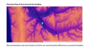
![A Sim le M del: O h g nal Lea S a e
O hogonal lea a e : D a a be - line be een all ime amp-poin of efe ence and me ma ind
peed ha minimi e he o hogonal di ance be een line and ime amp-poin
I [8]:
I look like e ha e a good amo n of da a (7k+ poin ) and a e pec able of 0.89. Le ' plo o line of
be !
'N da a ': 761,
' ff e ': 0.48915546304725566,
' 2': 0.8682745042710436,
' e': 0.7728460999482368
from b d.a a e.c e a import O a Lea S a e
# Re a le dail
da a_1D = da a. e a e('1D'). ea ()
_da a_1D = _da a['e a5_0']. e a e('1D'). ea ()
_ de = O a Lea S a e ( ef_ d= _da a_1D[' d'],
a e _ d=da a_1D[' d_58'],
a e a _ d='1D')
_ de . ()](https://image.slidesharecdn.com/predictingthewind-datascienceinwindresurceassessment-florianroscheck-201122042944/85/Predicting-the-Wind-Data-Science-in-Wind-Resource-Assessment-22-320.jpg)
![In [9]:
There is some sca er b model s he da a q i e ell.
O [9]:
l _m del. l ()](https://image.slidesharecdn.com/predictingthewind-datascienceinwindresurceassessment-florianroscheck-201122042944/85/Predicting-the-Wind-Data-Science-in-Wind-Resource-Assessment-23-320.jpg)
![P blem:
To make en e of he model in e m of ho ell i can p edic ind peed , e an o e i o
p edic he ind peed fo he ime pe iod hen e ha e me ma mea emen and hen compa e
he e mea emen o he model' p edic ion .
Fo hi p po e, a e o me ic i inapp op ia e - i ell no hing abo ind peed !
(In e p e a ion of i al o a he ick fo o hogonal lea a e eg e ion in gene al)
S l i n:
U e RMSE ( oo mean a e e o ) of p edic ed ind peed . ac al mea ed ind peed a e o me ic!
I [10]: # Define co ing me ic: RMSE
import as
def ( d c , ac a ):
return . ((( d c -ac a )**2). a ())
a _ d c =
a _ c =](https://image.slidesharecdn.com/predictingthewind-datascienceinwindresurceassessment-florianroscheck-201122042944/85/Predicting-the-Wind-Data-Science-in-Wind-Resource-Assessment-24-320.jpg)
![Le ' c e he im le h g nal lea a e m del ing RMSE!
In [11]:
The RMSE i 11% f he ind eed. Thi i n eall a g d n mbe . If e ld b ild he jec a ming
11% fa e ind han e ld ac all ha e, e ld ha e made a e e en i e mi ake.
S : H can e im e he m del?
Le ' lea n ab Ph ic !
RMSE of im le model: 0.315
RMSE a % of ind eed mean: 11%
edic ion = (ol _model. a am [' lo e']*l _da a_1D[' d']+ol _model. a am ['off e '])
all_ edic ion [' im le'] = edic ion
all_ co e [' im le'] = m e( edic ion, da a_1D[' d_58'])
in ('RMSE of im le model: :.3f '.fo ma (all_ co e [' im le']))
in ('RMSE a % of ind eed mean: :.0f %'.fo ma (all_ co e [' im le']/da a_1D[' d_58'].mean()*100))](https://image.slidesharecdn.com/predictingthewind-datascienceinwindresurceassessment-florianroscheck-201122042944/85/Predicting-the-Wind-Data-Science-in-Wind-Resource-Assessment-25-320.jpg)

![A Be e M del: Binned O h g nal Lea S a e
O r simple model j st binned in 12 direction sectors.
Q ick remark: We se for b ilding o r model here instead of , since I ant to sho o that
o can e en anal e ind data ith more common data science tools.
SciP Bright ind
In [12]: # B da a b d ec
dir_bin = pd.In er alInde .from_break (np.lin pace(0,360,13))
da a_1D = da a.re ample('1D').mean()
l _da a_1D = l _da a['era5_0'].re ample('1D').mean()
l _da a_1D['dir_bin'] = pd.c (l _da a_1D['dir'], dir_bin )
da a_1D['dir_bin'] = pd.c (da a_1D['dir'], dir_bin )](https://image.slidesharecdn.com/predictingthewind-datascienceinwindresurceassessment-florianroscheck-201122042944/85/Predicting-the-Wind-Data-Science-in-Wind-Resource-Assessment-29-320.jpg)
![I [13]:
RMSE f b ed de : 0.289
# B ild binned or hogonal lea q are model
from c . d import ODR, M de , Da a
def e _da a_ _d _b (d _b ):
_da a_ _b = _da a_1D[' d'][ _da a_1D['d _b '] == d _b ]
da a_ _b = da a_1D[' d_58'][da a_1D['d _b '] == d _b ]
ret rn _da a_ _b , da a_ _b
def de _fc (B, ):
ret rn B[0]* +B[1]
b _ a =
for b _ , d _b in e e a e(d _b ):
b _ a [b _ ] = ' _ a e ': None, 'be a ': None, ' e': . a , ' ed c ': None
_da a_ _b , da a_ _b = e _da a_ _d _b (d _b )
c c e _ = ( e ( _da a_ _b . de ). e ec ( e (da a_ _b . de )))
b _ a [b _ ][' _ a e '] = e (c c e _ )
if not c c e _ :
contin e
e = ODR(Da a( _da a_ _b [c c e _ ]. a e , da a_ _b [c c e _ ]. a e ), M de ( de _fc ),
be a0=[1., 0.5]). ()
b _ a [b _ ][' ed c '] = de _fc ( e .be a, _da a_ _b )
b _ a [b _ ]['be a '] = e .be a
b _ a [b _ ][' e'] = e(b _ a [b _ ][' ed c '], da a_ _b )
a _ ed c ['b ed'] = d.c ca ([b _ a [' ed c '] for b _ a in b _ a . a e ()
if b _ a [' ed c '] is not None]). _ de ()
a _ c e ['b ed'] = . a ea ([b _ a [' e'] for b _ a in b _ a . a e ()])
('RMSE f b ed de : :.3f '.f a (a _ c e ['b ed']))](https://image.slidesharecdn.com/predictingthewind-datascienceinwindresurceassessment-florianroscheck-201122042944/85/Predicting-the-Wind-Data-Science-in-Wind-Resource-Assessment-30-320.jpg)

![Fea e E gi ee i g
Let's come up ith some (simple) features that the random forest can feed on.
In [14]:
O [14]: d di d_ i g_3 d_ i g_5 d
i e
2018-02-01 1.455543 173.896001 15.397280 3.040377 3.040787 1.0 2.0
2018-02-02 1.528880 168.001625 16.170596 3.040377 3.040787 2.0 2.0
2018-02-03 2.025680 251.970139 16.567941 1.670035 3.040787 3.0 2.0
= da a_1D[' d_58']
# Ge c c e ime e
conc_inde = o ed(li ( e ( .inde ).in e ec ion(l _da a_1D.inde )))
X = l _da a_1D.loc[conc_inde ,[' d', 'di ', ' m ']]. o _inde ()
# R lli g mea
def make_ olling(da a, indo _ id h):
olling = da a[' d']. olling( indo _ id h).mean()
olling = olling.fillna( olling.mean())
olling.name = ' d_ olling_ '.fo ma ( indo _ id h)
return d.conca ([da a, olling], a i =1)
X = make_ olling(X, 3)
X = make_ olling(X, 5)
# Da e-ba ed fea e ca e em al a e
X.loc[conc_inde ,'d'] = X.inde .da
X.loc[conc_inde ,'m'] = X.inde .mon h
X.head(3)](https://image.slidesharecdn.com/predictingthewind-datascienceinwindresurceassessment-florianroscheck-201122042944/85/Predicting-the-Wind-Data-Science-in-Wind-Resource-Assessment-33-320.jpg)
![No that e ha e data ith features, let's build 2 models: One model for hich e ill ithhold some
alidation data and, for comparison ith the pre ious models, one model that uses all data.
I [15]:
The RMSE is not too high and de nitel ithin the range of the other models. Let's compare the models in
more detail.
RMSE (RF de , ai i g e ): 0.303
RMSE (RF de , a ida i e ): 0.330
RMSE (RF de , a da a): 0.300
f om k ea .e e b e impo Ra d F e Reg e
f om k ea . de _ e ec i impo ai _ e _ i
X_ ai , X_ a , _ ai , _ a = ai _ e _ i (X, , e _ i e=0.2, a d _ a e=42)
f_ de = Ra d F e Reg e ( _e i a =100, b_ c e=T e, a d _ a e=100, i _ a e _ eaf=10)
f_ de .fi (X_ ai , _ ai )
i ('RMSE (RF de , ai i g e ): :.3f '.f a ( e( f_ de . edic (X_ ai ), _ ai )))
i ('RMSE (RF de , a ida i e ): :.3f '.f a ( e( f_ de . edic (X_ a ), _ a )))
de = Ra d F e Reg e ( _e i a =100, b_ c e=T e, a d _ a e=100, i _ a e _ eaf=10)
de .fi (X, )
edic i = de . edic (X)
a _ edic i ['f e '] = d.Se ie ( edic i ,i de =c c_i de ). _i de ()
a _ c e ['f e '] = e( edic i , )
i ('RMSE (RF de , a da a): :.3f '.f a (a _ c e ['f e ']))](https://image.slidesharecdn.com/predictingthewind-datascienceinwindresurceassessment-florianroscheck-201122042944/85/Predicting-the-Wind-Data-Science-in-Wind-Resource-Assessment-34-320.jpg)
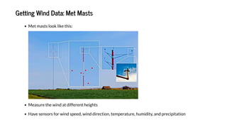
![Com a ing he 3 Wind S eed Model
I [16]:
All 3 models follo he arge mas nicel . The fores model some imes cap res peaks be er han o her
models (J n 18, Ma 6), b also occasionall has bigger misses (Apr 12, Ma 30).
from a ib impor a
d.Da aF a e(a _ edic i ). c['2018-04':'2018-06',:]. (fig i e=(25,5))
da a_1D[' d_58']. c['2018-04':'2018-06']. (c=' ', =2, abe ='Ta ge Ma ')
. ege d()
. h ()](https://image.slidesharecdn.com/predictingthewind-datascienceinwindresurceassessment-florianroscheck-201122042944/85/Predicting-the-Wind-Data-Science-in-Wind-Resource-Assessment-35-320.jpg)
![Time for a direct score comparison! Remember: The lo er the RMSE, the better the model.
I [17]:
Despite all the fanciness of the random forest model, it does not reach the score of our binned model. This
being said an RMSE of 0.3 is still relativel high hen measured in terms of ind speed.
.S (a _ c ). .ba ();](https://image.slidesharecdn.com/predictingthewind-datascienceinwindresurceassessment-florianroscheck-201122042944/85/Predicting-the-Wind-Data-Science-in-Wind-Resource-Assessment-36-320.jpg)
![An In-De h L k a he Binned M del
W e e b e b ed de , e d d e d a e ec . Le ' d a . We a
de a d b de . F , e ' d a e be f a e de ed e b .
In [18]:
6 b a e de 25 a e . F ed c e e b , e de bab e e ab e.
bin_ ise_params = pd.Series([stat['n_samples'] f stat in bin_stats.values()], inde =dir_bins)
bin_ ise_params.plot.bar(figsi e=(15,5))
plt.grid()](https://image.slidesharecdn.com/predictingthewind-datascienceinwindresurceassessment-florianroscheck-201122042944/85/Predicting-the-Wind-Data-Science-in-Wind-Resource-Assessment-37-320.jpg)
![I ld be be e e im le m del f he e ca e , ince e kn ha i ha been ained n a l f
da a and e f m ea nabl ell.
I [19]:
(0.0, 30.0]: Sim le m del
(30.0, 60.0]: Sim le m del
(60.0, 90.0]: Sim le m del
(90.0, 120.0]: Sim le m del
(120.0, 150.0]: Sim le m del
(150.0, 180.0]: Bi - i e m del
(180.0, 210.0]: Bi - i e m del
(210.0, 240.0]: Bi - i e m del
(240.0, 270.0]: Bi - i e m del
(270.0, 300.0]: Bi - i e m del
(300.0, 330.0]: Sim le m del
(330.0, 360.0]: Sim le m del
be a = []
fo be a, alid_bi ed, bi _ in i ([ a ['be a '] fo a in bi _ a . al e ()],
[ a [' _ am le ']>=25 fo a in bi _ a . al e ()],
di _bi ):
if no alid_bi ed:
be a .a e d( .a a a ([ l _m del. a am [' l e'], l _m del. a am [' ff e ']]))
i (' : Sim le m del'.f ma (bi _))
el e:
be a .a e d(be a)
i (' : Bi - i e m del'.f ma (bi _))](https://image.slidesharecdn.com/predictingthewind-datascienceinwindresurceassessment-florianroscheck-201122042944/85/Predicting-the-Wind-Data-Science-in-Wind-Resource-Assessment-38-320.jpg)
![No that e ha e a more rob st model, let's re-predict o r time series and check o r RMSE metric!
I [20]:
I [21]:
It looks as if lling the gaps in the binned model had a er bad impact on o r RMSE, making the ne model
the orst-performing one. What is going on here?
RMSE b ed - e de : 0.403
O [21]: b ed 0.289
e 0.300
e 0.315
b ed_ _ e 0.403
d e: a 64
b _ e = []
b _ ed c = []
f d _b , be a in (d _b , be a ):
_da a_ _b = _da a_1D[' d'][ _da a_1D['d _b '] == d _b ]
da a_ _b = da a_1D[' d_58'][ _da a_1D['d _b '] == d _b ]
b _ ed c = de _ c (be a, _da a_ _b )
b _ ed c .a e d(b _ ed c )
b _ e = e(b _ ed c , da a_ _b )
b _ e .a e d(b _ e)
a _ ed c ['b ed_ _ e'] = d.c ca (b _ ed c ). _ de ()
a _ c e ['b ed_ _ e'] = . a ea (b _ e )
('RMSE b ed - e de : :.3 '. a (a _ c e ['b ed_ _ e']))
d.Se e (a _ c e ). _ a e (). d(3)](https://image.slidesharecdn.com/predictingthewind-datascienceinwindresurceassessment-florianroscheck-201122042944/85/Predicting-the-Wind-Data-Science-in-Wind-Resource-Assessment-39-320.jpg)
![We sho ld look at the RMSE per bin to get a better pict re of ho hich binned model is to blame for the
increase in error.
In [22]:
We are getting the highest errors in the bins here e inserted the simple model.
B t, if there is no ind in those bins (= directions), the errors in those bins are not important!
What e reall need is a bin- eighted scoring metric!
pd.DataFrame( 'rmse': bin_rmses, 'n_samples': [stat['n_samples'] for stat in bin_stats. al es()] ,
inde =dir_bins).plot.bar(s bplots=Tr e,figsi e=(15,5));](https://image.slidesharecdn.com/predictingthewind-datascienceinwindresurceassessment-florianroscheck-201122042944/85/Predicting-the-Wind-Data-Science-in-Wind-Resource-Assessment-40-320.jpg)
![I ed Sc i g Me ic: Bi -Weigh ed RMSE
Fi , e i ca c a e he eigh e gi e each bi . Thi i i a he be f a e i
each bi .
In [23]:
N e ca b i d c i g f c i !
In [24]:
bin_n_samples = [s a ['n_samples'] f s a i bin_s a s. al es()]
bin_ eigh s = pd.Series(bin_n_samples, inde =dir_bins)/np.s m(bin_n_samples)
def rmse_binned(predic ion_spd, reference_spd, reference_dir):
sqr_errors = (predic ion_spd-reference_spd)**2
eigh s = bin_ eigh s[reference_dir]
error = np.sqr (np.nanmean(sqr_errors. al es* eigh s. al es))
e error](https://image.slidesharecdn.com/predictingthewind-datascienceinwindresurceassessment-florianroscheck-201122042944/85/Predicting-the-Wind-Data-Science-in-Wind-Resource-Assessment-41-320.jpg)
![Wi h he c i g f c i de be , e ' ca c a e he bi - eigh ed RMSE f a f de '
edic i .
I [25]:
The bi - eigh ed RMSE h c ea e diffe e ce be ee he de ha he eigh ed c e:
O bi ed de ha i i g he i e de ' i f a i i ga c e be
O i e de e f e ha he bi ed de
O f e de e f
S , af e a , e d e b b ed de ed c g- e d eed a a !
O [25]: U e g ed B -We g ed
b ed_ _ e 0.4026 0.1328
b ed 0.2888 0.1347
e 0.3152 0.1416
f e 0.2996 0.1807
a _ c e _b ed =
f de _ a e, ed c _ d in a _ ed c . e ():
da a_1D[' d_58'][da a_1D['d _b '] == d _b ]
a _ c e _b ed[ de _ a e] = e_b ed( ed c _ d, _da a_1D[' d'], _da a_1D['d '])
d.Da aF a e([a _ c e , a _ c e _b ed]).T. e a e(c = 0: 'U e ed', 1: 'B -We ed' )
. _ a e ('B -We ed'). e.ba ( =0, a =0.5, c =' b e').f a (' :.4f ')](https://image.slidesharecdn.com/predictingthewind-datascienceinwindresurceassessment-florianroscheck-201122042944/85/Predicting-the-Wind-Data-Science-in-Wind-Resource-Assessment-42-320.jpg)
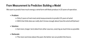
![P edic ing he Long-Te m Wind S eed
No e can predict the long-term ind speed at our site. This helps us to get a good idea of ho much ind
energ e can potentiall harvest if e build a ind turbine there.
Remember: We assume the ind in the future ill behave like the ind in the past. To get to the long-term
ind speed, e take all predictions from our bin_fill_ im le model. To ma imi e accurac , e
substitute it ith actual measurements from our mast herever possible.
I [26]:
Let's summari e our long-term ind speed time series!
I [27]:
R a 761 - a a a a (10.3%).
S a : 1999-12-31, L : 20 a , A . 2.86 /
_ _a _ a = a _ ['b _ _ ']
_ _a _ a [ a a_1D[' _58']. ] = a a_1D[' _58']
('R a - a a a a ( :.1% ).'
. a ( a a_1D. a [0], a a_1D. a [0]/ _ _a _ a . a [0]))
('S a : :%Y-% -% , L : :.0 a , A . :.2 / '
. a ( _ _a _ a . [0], _ _a _ a . a [0]/(365.25), _ _a _ a . a ()))](https://image.slidesharecdn.com/predictingthewind-datascienceinwindresurceassessment-florianroscheck-201122042944/85/Predicting-the-Wind-Data-Science-in-Wind-Resource-Assessment-43-320.jpg)
![Le ' nd he hear e ponen b ing S ea .A e age() me hod.brigh ind'
In [28]:
Shea e nen : 0.19
anem me e _heigh = [30, 45, 58]
a e age_ hea = b .Shea .A e age(da a[anem me e ], anem me e _heigh )
in ('Shea e nen : :.3 '.f ma (a e age_ hea .al ha))](https://image.slidesharecdn.com/predictingthewind-datascienceinwindresurceassessment-florianroscheck-201122042944/85/Predicting-the-Wind-Data-Science-in-Wind-Resource-Assessment-49-320.jpg)
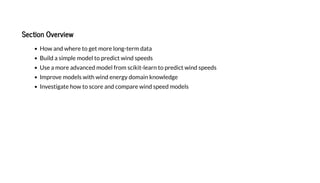
![Appl Shea La o Long-Te m Time Se ie
N ha e kn he hea e nen , e can calc la e he l ng- e m ime e ie a bine heigh .
In [29]:
On a e age, he ind i 9.1% fa e a he bine heigh han a he mea ed heigh .
h_ bine 100.0 + 119.0
h_ma 80.0 + 58.0
l _ eed_a _ bine l _ eed_a _ma *(h_ bine/h_ma )**a e age_ hea .al ha
in ('On a e age, he ind i :.1% fa e a he bine heigh han a he mea ed heigh .'
.fo ma (l _ eed_a _ bine.mean()/l _ eed_a _ma .mean()-1))](https://image.slidesharecdn.com/predictingthewind-datascienceinwindresurceassessment-florianroscheck-201122042944/85/Predicting-the-Wind-Data-Science-in-Wind-Resource-Assessment-50-320.jpg)

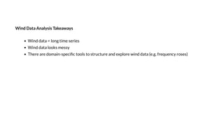
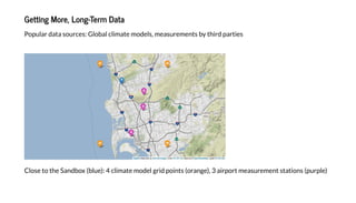
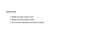
![Po er Curve
Po er C r e: T rbine po er o tp t as f nction of ind speed. Let's plot the V112 po er c r e!
I [30]:
Obser ations: T rbine onl starts to prod ce po er at abo t 2 m/s ind speed, po er o tp t is stead
bet een ca. 12 and 25 m/s.
e _c e = d. ead_c ('./da a/ e a _ 112_ e _c e.c ', i de _c =0).i c[:,0]
e _c e.i de . a e = 'Wi d S eed [ / ]'
e _c e. ( i e='Ve a V112 P e C e (P e O i kW)', fig i e=(15,5), i =(0,3500));](https://image.slidesharecdn.com/predictingthewind-datascienceinwindresurceassessment-florianroscheck-201122042944/85/Predicting-the-Wind-Data-Science-in-Wind-Resource-Assessment-52-320.jpg)
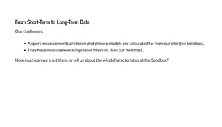
![Po er C r e s. Predicted Wind Speed
No that e kno ho much po er the V112 turbine produces b ind speed, let's see ho our predicted
long-term ind speed ts into the picture.
I [53]:
Obser ations: Long-term ind speed is er small in comparison to hat the turbine can handle, the V112
turbine is completel o ersi ed for this site!
e _c e. ( e='Ve a V112 P e C e (P e O W) . L -Te W d S eed')
_ eed_a _ b e. . ( ec da _ =Tr e, a a=0.5, b =20 , f e=(15,5), abe =' - e ');](https://image.slidesharecdn.com/predictingthewind-datascienceinwindresurceassessment-florianroscheck-201122042944/85/Predicting-the-Wind-Data-Science-in-Wind-Resource-Assessment-53-320.jpg)
![Calculating Po er Output
De i e he V112 being e i ed, le ' la a nd i h he ene g d c i n n mbe e ld ge if
e e e b ild hi bine. We an ge a "feel" f he e and i in he c n e f he
c mm ni a nd he Sandb , i e.
I [78]:
Alm 25 MWh! I ha a l ? I ha a li le? Le ' e e hi n mbe in he e m :
I [79]:
Tha i a l f a and a g d am n f elec ic ca cha ge !
Mea b e e ea W : 24,925
T a ab e a e da f 1 ea : 975
F Te a M de S c a e e ea : 249
_ e _ . e ( _ eed_a _ b e, e _c e. de , e _c e. a e , ef 0, 0)
_ e _ d.Se e ( _ e _ , de _ eed_a _ b e. de )
e_ e e _d a _ ea _ e _ . a e[0]/(365.25)
_ e _ ea _ e _ . ()/ e_ e e _d a _ ea
('Mea b e e ea W : :,.0f '.f a ( _ e _ ea ))
(' T a ab e a e da f 1 ea : :.0f '.f a ( _ e _ ea /(3.5/60*1.2)/365.25))
(' F Te a M de S c a e e ea : :.0f '.f a ( _ e _ ea /100))](https://image.slidesharecdn.com/predictingthewind-datascienceinwindresurceassessment-florianroscheck-201122042944/85/Predicting-the-Wind-Data-Science-in-Wind-Resource-Assessment-54-320.jpg)
![Ho Man Ho seholds Co ld We Po er?
2017: T e ea Sa D e e d c ed 5600 W f e ec c ( ce:
).
T e Sa db ZIP c de (92121) ad 1677 e d 2010 ( ce: ).
SDGE a E
P ec
-c de .c
I [97]:
We , a e a d eadf ce a . B , ad , d ea e e a e a c a . T ea : We
d ' ea a b e d a e e Sa D e e d .
C ea , e e a c a da a, b d a d b e c e e Sa db d e a e e e.
W e bad - aced b e, e c d e 4.5 Sa D e e d (0.3% a a d e Sa db ).
W 377 bad - aced b e , e c d e 1678 Sa D e e d (100.1% a a d e Sa db ).
e d _ e _ b e _ e _ ea /5600
c _ _92121_ e _ b e e d _ e _ b e/1677
('W e bad - aced b e, e c d e :.1 Sa D e e d ( :.1% a a d e Sa db ).'
. a ( e d _ e _ b e, c _ _92121_ e _ b e))
('W 377 bad - aced b e , e c d e :.0 Sa D e e d ( :.1% a a d e Sa db ).'
. a ( e d _ e _ b e*377, c _ _92121_ e _ b e*377))](https://image.slidesharecdn.com/predictingthewind-datascienceinwindresurceassessment-florianroscheck-201122042944/85/Predicting-the-Wind-Data-Science-in-Wind-Resource-Assessment-55-320.jpg)
![N Ca ac Fac (NCF)
E e mea e h ell a bine a ind eed di ib i n and elec ici g id en i nmen in e m
f ne ca aci fac (NCF).
Thi me ic de c ibe h m ch elec ici he bine ill gene a e f m he ac al ind en i nmen , in
c m a i n h m ch i c ld he e icall gene a e, if he ind ble en gh make he bine
gene a e i ma im m e all he ime.
In [100]:
Thi ne ca aci fac i eall , eall l ! (T ical NCF : 30% - 50%)
We c ld lace hi bine in a be e !
N b d ld b ild a bine cl e he Sandb (gi en a i cal da a)!
The net capacit factor is 2.2%.
ncf output_per_ ear/(365.25*po er_cur e.ma ())
print('The net capacit factor is :.1% .'.format(ncf))](https://image.slidesharecdn.com/predictingthewind-datascienceinwindresurceassessment-florianroscheck-201122042944/85/Predicting-the-Wind-Data-Science-in-Wind-Resource-Assessment-56-320.jpg)

![Let's plot our diurnal pro le to see if we would produce a good amount of electricty during these pro table
hours.
I [108]:
Unfortunately, it looks as if we produce power right when a lot of solar power is in the grid, pushing
electricity prices down. Not every wind project is like this – sometimes wind speeds are high just as energy
demand peaks.
mea ed_da a = da a[' d_58']. e am le('1h').mea ()
mea ed_da a.g b (mea ed_da a.i de .h ).mea ()
. l (fig i e=(15,5), i le='Di al P e P d c i P file', lim=(0,23));](https://image.slidesharecdn.com/predictingthewind-datascienceinwindresurceassessment-florianroscheck-201122042944/85/Predicting-the-Wind-Data-Science-in-Wind-Resource-Assessment-58-320.jpg)
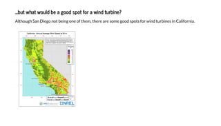


El documento discute técnicas de ciencia de datos para predecir el comportamiento de la energía eólica utilizando análisis estadísticos y modelos predictivos. Se enfatiza la importancia de recopilar datos a largo plazo para mejorar la precisión de las predicciones sobre la generación de electricidad a partir del viento en un periodo de 25 años. Se presentan desafíos relacionados con la confianza en las mediciones del clima y la utilidad de modelos avanzados como el regresor de bosque aleatorio para mejorar la estimación de los parámetros del viento.