The document discusses potential flow modeling of ducted propellers with blunt trailing edges, utilizing a panel method to evaluate pressure distributions and forces. The study investigates the applicability of the Kutta condition in modeling flows and assesses grid convergence and pressure distributions based on various configurations and trailing edge shapes. Results include numerical analyses and comparisons with experimental data, indicating the effectiveness of the proposed modeling approach for different duct and propeller systems.

1. Sixth International Symposium on Marine Propulsors – SMP19
26-30 May 2019, Rome, Italy
Potential Flow Modelling of Ducted
Propellers with Blunt Trailing Edge Duct
Using a Panel Method
J. Baltazar, J.A.C. Falcão de Campos
Marine Environment and Technology Center (MARETEC),
Instituto Superior Técnico (IST), University of Lisbon, Portugal

2. Outline
• Motivation and Objectives
• Potential Modelling of Blunt Trailing Edges
• Panel Method
• Flow model
• Wake alignment
• Numerical Kutta condition
• Results
• Ducted propeller
• Grid convergence study
• Influence of the Kutta condition
• Pressure distribution on the duct
• Propeller and duct forces
• Concluding Remarks
smp´19, Rome, Italy 2
May 2019

3. Motivation
• Hypothesis: Can the duct circulation can be modelled by a suitable application of the Kutta
condition in combination with some potential flow model for separated flow from the blunt
trailing edge?
• Then it would be possible to model the ducted propeller flow with a potential panel code with a
reasonable assessment of pressure distributions and forces.
• For the Duct 19A a simple form of the pressure Kutta condition applied at “geometry dominated”
separation points from the trailing edge enabled a reasonable modelling of the Ka 4.70 ducted
propeller system for predicting pressure and forces (Baltazar et al, 2015)
• Can this approach be extended to ducts with thicker round trailing edges with “flow dominated”
separation?
smp´19, Rome, Italy 3
May 2019

4. Objectives
smp´19, Rome, Italy 4
May 2019
• Investigate the application of a simple and practical form of the Kutta condition with
a potential panel code for the duct 37 with a thick blunt trailing edge.
• Perform RANSE calculations for the same configuration to investigate on more physical
grounds the adequacy of the previous approach.
• Investigate if the potential panel code modelling can be applied for different propellers
inside the duct 37.

5. Potential Flow Modelling for Blunt Trailing Edges
• Classical Models: Cavity and Wake theory
smp´19, Rome, Italy 5
May 2019
Illustration of 2D separation bubbles
M.J. Lighthill, 1963
Illustration of separation bubbles on
Duct 37 in uniform flow based on paint
tests, JAC Falcão de Campos, 1983

6. Flow on Duct Blunt Trailing Edges with RANS
• Bosschers et al, smp´15 (2015)
smp´19, Rome, Italy 6
May 2019
• Kinnas et al, smp’13 (2013)
Hoekstra (2006)
Duct 19A
Duct 19A
Streamline pattern near the t.e. of
Duct 19A in axisymmetric flow
calculated with RANS, M. Hoekstra,
2006

7. Kutta Condition for Blunt Trailing Edges
• Modified Geometry with Sharp Trailing Edge
• Extension of Trailing Edge:
• Foils: Pan & Kinnas (2009) “A Viscous/Inviscid Interactive Approach and its Application to Hydrofoils and Propellers with
Non-Zero Trailing Edge Thickness” SMP’09, Trondheim, Norway, June 2009.
• Ducts: Kinnas et al (2013), “Prediction of the Unsteady Cavitating Performance of Ducted Propellers Subject to Inclined
Inflow”, SMP’13, Launceston, Tasmania, May 2013.
• Modified Duct Geometry
• Baltazar et al (2011), “Open Water Thrust and Torque Predictions of a Ducted Propeller System in Open Water”, SMP’11,
Hamburg, Germany, June 2011.
• Pressure Kutta Condition at Flow Separation Points
• “Geometry dominated” (Duct 19A)
• Baltazar et al (2015), “Potential Flow Modelling of Ducted Propellers With a Panel Method”, SMP’15, Austin, USA, June
2015.
• “Flow dominated” (Duct 37)
smp´19, Rome, Italy 7
May 2019

8. Panel Method
• Potential low order panel method based on Morino formulation
• Flow Modelling
• Closed Gap: Baltazar et al (2011)
• Wake Alignment: Baltazar et al (2011)
• Iterative propeller wake pitch alignment downstream of blade trailing edge
• Propeller wake contraction neglected
• Kutta Condition: Baltazar et al (2015)
• Iterative pressure Kutta condition at specified Kutta points
• Pressure constant downtream of Kutta points
• No viscous drag corrections.
smp´19, Rome, Italy 8
May 2019

9. Ducted Propeller: Propeller 4902 in Duct 37
smp´19, Rome, Italy 9
May 2019
G1

10. Ducted Propeller: Propeller 4902 in Duct 37
smp´19, Rome, Italy 10
May 2019
X
Y

11. Results: Grid Convergence Study
smp´19, Rome, Italy 11
May 2019
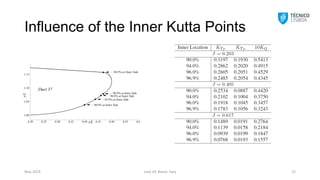
Kutta points at 96.9%
r/R
(
R
2
)
0.3 0.4 0.5 0.6 0.7 0.8 0.9 1.0
-0.03
0.00
0.03
0.06
0.09
G4
G3
G2
G1
Blade Circulation
J=0.203
J=0.405
J=0.617
Position between blades [deg.]
(
R
2
)
0 10 20 30 40 50 60 70 80 90
0.15
0.20
0.25
0.30
0.35
0.40 G4
G3
G2
G1
Duct Circulation
J=0.617
J=0.203
J=0.405
x/L
y/L
0.20 0.25 0.30 0.35 0.40 0.45 0.50 0.55 0.60
1.00
1.05
1.10
1.15
Duct 37
94.0%
99.5%
99.0%
96.9%
96.0%
98.0%

12. Influence of the Inner Kutta Points
smp´19, Rome, Italy 12
May 2019
x/L
y/L
0.20 0.25 0.30 0.35 0.40 0.45 0.50 0.55 0.60
1.00
1.05
1.10
1.15
Duct 37
90.0% at Inner Side
96.9% at Outer Side
96.9% at Inner Side
96.0% at Inner Side
94.0% at Inner Side

13. Duct Pressure Distribution – Mean Pressure
smp´19, Rome, Italy 13
May 2019
Equation (3)
s/L
-C
p
(0)
J
2
/2
0.0 0.2 0.4 0.6 0.8 1.0
0.0
0.5
1.0
1.5
Panel Method: Inner 90.0%, Outer 96.9%
Panel Method: Inner 94.0%, Outer 96.9%
Panel Method: Inner 96.9%, Outer 96.9%
RANS (Haimov et al, 2011)
Experimental (Cruijff et al, 1980)
J=0.203
s/L
-C
p
(0)
J
2
/2
0.0 0.2 0.4 0.6 0.8 1.0
0.0
0.5
1.0
1.5
Panel Method: Inner 90.0%, Outer 96.9%
Panel Method: Inner 94.0%, Outer 96.9%
Panel Method: Inner 96.9%, Outer 96.9%
RANS (Haimov et al, 2011)
Experimental (Cruijff et al, 1980)
J=0.405
s/L
-C
p
(0)
J
2
/2
0.0 0.2 0.4 0.6 0.8 1.0
0.0
0.5
1.0
1.5
Panel Method: Inner 90.0%, Outer 96.9%
Panel Method: Inner 94.0%, Outer 96.9%
Panel Method: Inner 96.9%, Outer 96.9%
RANS (Haimov et al, 2011)
Experimental (Cruijff et al, 1980)
J=0.617

14. Duct Pressure Distribution – Higher
Harmonics
smp´19, Rome, Italy 14
J=0.203
J=0.405
J=0.617
May 2019
s/L
C
p
(1)
J
2
/2
0.0 0.2 0.4 0.6 0.8 1.0
0.0
0.2
0.4
0.6
0.8
Panel Method: Inner 90.0%, Outer 96.9%
Panel Method: Inner 94.0%, Outer 96.9%
Panel Method: Inner 96.9%, Outer 96.9%
Experimental (Cruijff et al, 1980)
1st Harmonic
s/L
C
p
(1)
J
2
/2
0.0 0.2 0.4 0.6 0.8 1.0
0.0
0.2
0.4
0.6
Panel Method: Inner 90.0%, Outer 96.9%
Panel Method: Inner 94.0%, Outer 96.9%
Panel Method: Inner 96.9%, Outer 96.9%
Experimental (Cruijff et al, 1980)
1st Harmonic
s/L
C
p
(1)
J
2
/2
0.0 0.2 0.4 0.6 0.8 1.0
0.0
0.1
0.2
0.3
0.4
0.5
Panel Method: Inner 90.0%, Outer 96.9%
Panel Method: Inner 94.0%, Outer 96.9%
Panel Method: Inner 96.9%, Outer 96.9%
Experimental (Cruijff et al, 1980)
1st Harmonic
s/L
C
p
(2)
J
2
/2
0.0 0.2 0.4 0.6 0.8 1.0
0.0
0.1
0.2
0.3
0.4
0.5
Panel Method: Inner 90.0%, Outer 96.9%
Panel Method: Inner 94.0%, Outer 96.9%
Panel Method: Inner 96.9%, Outer 96.9%
Experimental (Cruijff et al, 1980)
2nd Harmonic
s/L
C
p
(2)
J
2
/2
0.0 0.2 0.4 0.6 0.8 1.0
0.0
0.1
0.2
0.3
0.4
Panel Method: Inner 90.0%, Outer 96.9%
Panel Method: Inner 94.0%, Outer 96.9%
Panel Method: Inner 96.9%, Outer 96.9%
Experimental (Cruijff et al, 1980)
2nd Harmonic
s/L
C
p
(2)
J
2
/2
0.0 0.2 0.4 0.6 0.8 1.0
0.0
0.1
0.2
0.3
Panel Method: Inner 90.0%, Outer 96.9%
Panel Method: Inner 94.0%, Outer 96.9%
Panel Method: Inner 96.9%, Outer 96.9%
Experimental (Cruijff et al, 1980)
2nd Harmonic
s/L
C
p
(3)
J
2
/2
0.0 0.2 0.4 0.6 0.8 1.0
0.0
0.1
0.2
0.3
0.4
0.5
Panel Method: Inner 90.0%, Outer 96.9%
Panel Method: Inner 94.0%, Outer 96.9%
Panel Method: Inner 96.9%, Outer 96.9%
Experimental (Cruijff et al, 1980)
3rd Harmonic
s/L
C
p
(3)
J
2
/2
0.0 0.2 0.4 0.6 0.8 1.0
0.0
0.1
0.2
0.3
Panel Method: Inner 90.0%, Outer 96.9%
Panel Method: Inner 94.0%, Outer 96.9%
Panel Method: Inner 96.9%, Outer 96.9%
Experimental (Cruijff et al, 1980)
3rd Harmonic
s/L
C
p
(3)
J
2
/2
0.0 0.2 0.4 0.6 0.8 1.0
0.0
0.1
0.2
Panel Method: Inner 90.0%, Outer 96.9%
Panel Method: Inner 94.0%, Outer 96.9%
Panel Method: Inner 96.9%, Outer 96.9%
Experimental (Cruijff et al, 1980)
3rd Harmonic
s/L
C
p
(4)
J
2
/2
0.0 0.2 0.4 0.6 0.8 1.0
0.0
0.1
0.2
0.3
0.4
Panel Method: Inner 90.0%, Outer 96.9%
Panel Method: Inner 94.0%, Outer 96.9%
Panel Method: Inner 96.9%, Outer 96.9%
Experimental (Cruijff et al, 1980)
4th Harmonic
s/L
C
p
(4)
J
2
/2
0.0 0.2 0.4 0.6 0.8 1.0
0.0
0.1
0.2
0.3
Panel Method: Inner 90.0%, Outer 96.9%
Panel Method: Inner 94.0%, Outer 96.9%
Panel Method: Inner 96.9%, Outer 96.9%
Experimental (Cruijff et al, 1980)
4th Harmonic
s/L
C
p
(4)
J
2
/2
0.0 0.2 0.4 0.6 0.8 1.0
0.00
0.05
0.10
0.15
Panel Method: Inner 90.0%, Outer 96.9%
Panel Method: Inner 94.0%, Outer 96.9%
Panel Method: Inner 96.9%, Outer 96.9%
Experimental (Cruijff et al, 1980)
4th Harmonic

15. Blade Pressure Distribution
smp´19, Rome, Italy 15
May 2019
s/c
C
p
0.0 0.2 0.4 0.6 0.8 1.0
-2.5
-2.0
-1.5
-1.0
-0.5
0.0
0.5
1.0
Panel Method: Inner 90.0%, Outer 96.9%
Panel Method: Inner 94.0%, Outer 96.9%
Panel Method: Inner 96.9%, Outer 96.9%
J=0.203
s/c
C
p
0.00 0.02 0.04 0.06
-3.0
-2.0
-1.0
0.0
1.0
s/c
C
p
0.0 0.2 0.4 0.6 0.8 1.0
-2.0
-1.5
-1.0
-0.5
0.0
0.5
1.0
Panel Method: Inner 90.0%, Outer 96.9%
Panel Method: Inner 94.0%, Outer 96.9%
Panel Method: Inner 96.9%, Outer 96.9%
J=0.405
s/c
C
p
0.00 0.02 0.04 0.06
-2.0
-1.0
0.0
1.0
s/c
C
p
0.0 0.2 0.4 0.6 0.8 1.0
-1.0
-0.5
0.0
0.5
1.0
Panel Method: Inner 90.0%, Outer 96.9%
Panel Method: Inner 94.0%, Outer 96.9%
Panel Method: Inner 96.9%, Outer 96.9%
J=0.617
s/c
C
p
0.00 0.02 0.04 0.06 0.08
-1.0
-0.5
0.0
0.5
r/R=0.90

16. Ducted Propeller Thrust and Torque
smp´19, Rome, Italy 16
May 2019
J
0.1 0.2 0.3 0.4 0.5 0.6 0.7 0.8
-0.1
0.0
0.1
0.2
0.3
0.4
Panel Method, Inner: 90.0%, Outer: 96.9%
Panel Method, Inner: 94.0%, Outer: 96.9%
Panel Method, Inner: 96.9%, Outer: 96.9%
Experiments (Cruijff et al, 1980)
KT
KT
D
P
Propeller and Duct Thrust
J
0.1 0.2 0.3 0.4 0.5 0.6 0.7 0.8
-0.1
0.0
0.1
0.2
0.3
0.4
0.5
0.6
0.7
Panel Method, Inner: 90.0%, Outer: 96.9%
Panel Method, Inner: 94.0%, Outer: 96.9%
Panel Method, Inner: 96.9%, Outer: 96.9%
Experiments (Cruijff et al, 1980)
10KQ
Propeller Torque

17. Concluding Remarks
• The application of a simple Kutta condition to the duct 37 with a round thick trailing edge has
been investigated with a panel method.
• The duct loading is adjusted by specifying the position of the Kutta points on the inner surface
intending to simulate the flow separation location from the trailing edge.
• The results were compared with measurements of the ducted propeller forces and inner duct
pressure.
• As expected, there a significant effect of the location of the inner Kutta points on the predicted
forces and mean pressure. The effect is much larger on the propeller thrust than on the duct
thrust.
• The correlation on pressure and propeller forces with the experimental data at increasing loading
improves when displacing the inner kutta point toward the trailing edge.
• The method appears to capture reasonably the (low) higher harmonics in the duct inner pressure
as they are potential flow dominated.
smp´19, Rome, Italy 17
May 2019

18. Aknowledgement
• The authors would like to acknowledge the permission of
MARIN to share the experimental data used in the
comparisons presented in this study.
smp´19, Rome, Italy 18
May 2019
Thank you