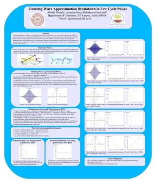
Rotating Wave Approximation (RWA) breaks down for few-cycle pulses. Using Gaussian pulses, quantum logic gates like NOT and Hadamard can be implemented, but their effectiveness decreases for pulses with a small frequency compared to the transition frequency between levels. Attosecond pulses cannot be used to study ultrafast phenomena in biology due to limitations of RWA - the required x-ray or gamma ray frequencies would damage living cells. The document examines how RWA breakdown affects population dynamics in a two-level system interacting with femtosecond and attosecond pulses.

1. Rotating Wave Approximation Breakdown in Few Cycle Pulses
Abhijit Mondal, Amartya Bose, Debabrata Goswami*
Department of Chemistry, IIT Kanpur, India-208016
*Email: dgoswami@iitk.ac.in
Abstract
Though population evolution with pulsed laser interaction has been very successful with the help of RWA,
however, for a few cycle pulses, the RWA breaks down. This poster elucidates this work mathematically for
model systems. In this poster we have shown how gaussian pulses are used to produce NOT gate and
Hadamard gate, how ineffective the Gate operation becomes in the regime of small electric field frequency of
the gaussian pulse and how ineffective can such short pulses(attosecond) be when it comes to applications in
biology and chemistry.
Attosecond Pulses
Pulses of the order of 10-18s fall into the attosecond domain. Such short pulses are invaluable for probing the
dynamics of fast systems. Electronic motion occur in the sub-femtosecond to a few femtosecond timescales.
Hence, in the attosecond domain, electronic motion appears frozen.
Electric field, avg. electric field vs. ω and population dynamics of levels 1 and 2 for ω = 1000
rad fs-1 and 4 fs pulse.
Rotating Wave Approximation(RWA)
The time dependent electric field of a light pulse having a Gaussian profile is given as:
E(t) = exp(-αt2) ( exp(-iωt) + exp(iωt) )
Interaction of this field with an isolated 2-level system, gives the Hamiltonian of the system which has the
terms exp(-i(ω-ω0)t ) and also the term exp(-i(ω+ω0)t ) in it.
For population inversion in 2-level sytems ω = ω0, and thus the 1st term becomes 1, but the second term Electric field, avg. electric field vs. ω and population dynamics of levels 1 and 2 for ω = 1000
becomes exp(-i(2ω)t ). Now if ω is large enough then the temporal average of the electric field over the rad fs-1 and 1.5 fs pulse.
pulse duration becomes 0, so we can neglect this term, but if ω is small then the temporal average will not
be 0, hence RWA breaks down.
Electric field for femtosecond pulse Electric field for attosecond pulse Electric field, avg. electric field vs. ω and population dynamics of levels 1 and 2 for ω = 1000
rad fs-1 and 0.5 fs pulse.
Limitations on Attosecond Pulses based on RWA

Atleast 1.5 oscillations are required in the pulse duration for the RWA to be valid for a pulse.

Assuming that the duration of the pulse is 1 attosecond and 1.5 oscillations are present in that duartion,
then frequency of the electric field is 1.5 rad ats-1 = 1.5*1018 rad s-1. Thus the wavelength of the light
required will be around c/ω = 2*10-10 m = 2 Å.

Wavelength of 2 Å is for X-rays and gamma rays. Thus to freeze the motion of electrons to observe it
using a light pulse of attosecond duration, we need x-rays or gamma rays as the light source.

Using x-rays and gamma rays for observing fast phenomenon in biological living systems would damage
living cells and could be harmful in the long term. Thus we cannot use attosecond pulses to detect very
fast molecular phenomenons in living cells.
Two level system population dynamics Electric field, avg. electric field vs. ω and population dynamics of levels 1 and 2 for ω = 1000
 ∂c1(t)/∂t = (i/2)ωR(exp(i(ω-ω0)t ) + exp(-i(ω+ω0)t ) c2(t) rad fs-1 and 0.08 fs= 80 ats pulse.
 ∂c (t)/∂t = (i/2)ω (exp(-i(ω-ω )t ) + exp(i(ω+ω )t ) c (t)
2 R 0 0 1
 ω (t) (rabi frequency) = μ exp(-αt2)/ ħ
R 12
 μ is the transition dipole moment from level 1 to level 2.
12
Quantum NOT Gate using gaussian Quantum Hadamard Gate using
3π pulse laser pulse gaussian 3π/2 laser pulse
Electric field, avg. electric field vs. ω and population dynamics of levels 1 and 2 for ω = 1000
rad fs-1 and 0.02 fs = 20 ats pulse.
Acknowledgement
On application of the 3π gaussian pulse, the On application of the 3π/2 gaussian pulse, both the 
We would like to thank DST, CSIR, New Delhi (India ) for their generous funding.
excited state population becomes saturated at the ground state and excited state population saturates at 
Wellcome Trust (UK).
expense of the ground state population half the total population 
To all the Group members of Dr. Goswami's lab