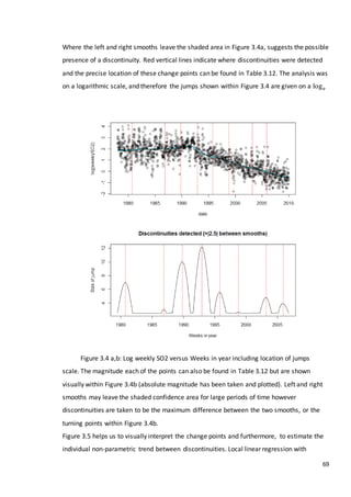
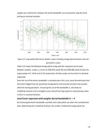
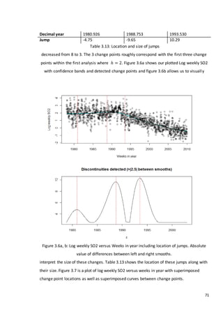
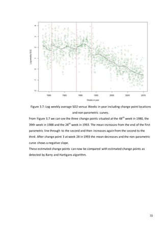
Statistical Tools in Environmental
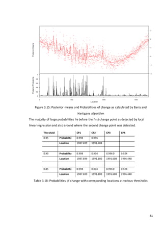
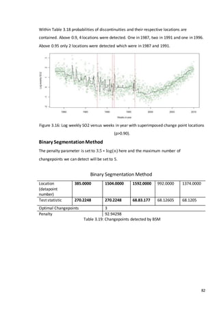
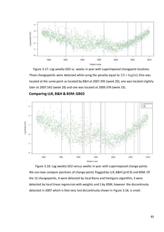
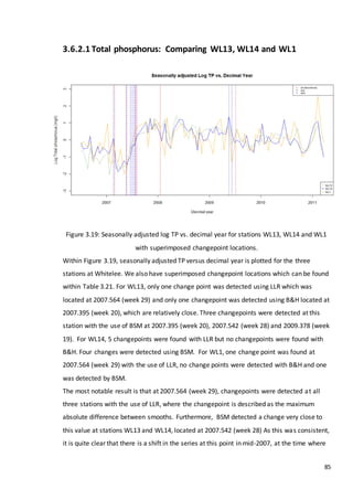
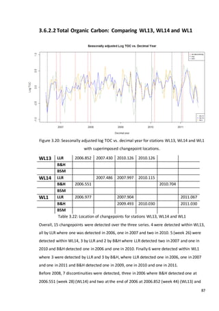
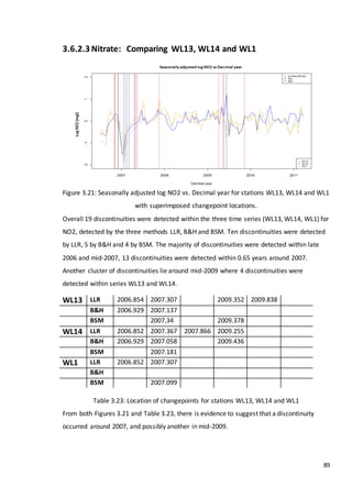
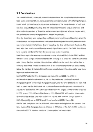
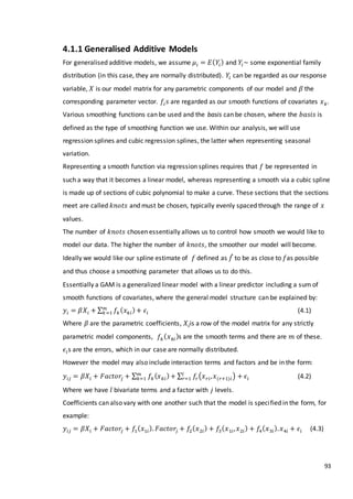
Impact Assessment
Fraser Tough
A Dissertation Submitted to the
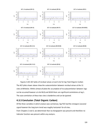
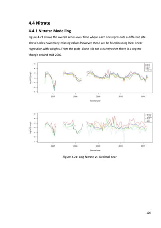
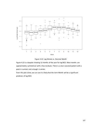
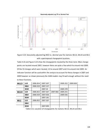
University of Glasgow
for the degree of
Master of Science
School of Mathematics & Statistics
May 2013
©Fraser Tough, May 2013
i
Abstract
Environmental Impact Assessment consists of assessing the possible effects of a project of
development on the environment. Statistical methods which are used in this process include
those with the ability to detect the magnitude of an impact at the time in which an
intervention has occurred, and the ability to detect when an intervention has occurred if the
time of impact is not available. The impact at the time at which the intervention has
occurred is also known as a ‘changepoint’. This project consists of evaluating methods used
to assess the magnitude of these ‘impacts’, and the methods which can be used to
determine where an impact has occurred if the time of impact is not available.
A number of datasets have been made available for analysis within this thesis, each of these
datasets are expected to contain impacts within them. By reviewing the techniques and
methods which are available for statisticians, applications to these datasets were made.
The classic approach to quantifying the magnitude of change within a series when the time
of the impact is known is Before-After-Control-Impact (BACI) design, which uses a dummy
variable within a linear regression model to determine whether a significant change in mean
can be detected. This thesis reviewed the history and the approaches used by statisticians
when using this method, and the adaptions that can be made. BACI was then applied to our
own datasets to determine whether a significant change in mean could be detected.
Many statistical changepoint detection methods are available to statisticians when the
location of a changepoint, if any, is not known. By summarising the methods available and
calculating the power of various methods via a simulation study, a number of changepoint
detection methods were applied to real life data.
Finally, various modelling techniques were applied to the available datasets and by
incorporating terms to indicate the detected location of changepoints, we could determine
whether adding these terms gives better fitting models.
ii
Acknowledgements
First and foremost I would like to thank Marian Scott OBE for her supervision, support and
encouragement throughout the writing of my thesis. Without her help, knowledge,
comments and suggestions this thesis would not have been possible.
Many thanks go out to Susan Waldron for her help and advice as well as Helen Murray for
collecting the samples at Whitelee windfarm.
I would also like to thank the Information Services Division for their generous funding, and
the department of Statistics at the University of Glasgow for acquiring this funding.
iii
Contents
Abstract........................................................................................................................................i
Acknowledgements .....................................................................................................................ii
List of figures.............................................................................................................................. vi
List of tables................................................................................................................................ x
1 Introduction to Changepoint Analysis and its applications.......................................................... 1
1.1 What is Environmental Impact Assessment........................................................................... 1
1.2 What is an ‘Impact’ and types of impact............................................................................... 3
1.3 Application of techniques.................................................................................................... 6
1.3.1 Overview...................................................................................................................... 6
1.3.2 European Monitoring and Evaluation Programme (EMEP)............................................... 6
1.3.3 Whitelee wind farm...................................................................................................... 8
1.4 Aim of this work.................................................................................................................12
2 Before After Control Impact (BACI) design ................................................................................14
2.1 An introduction to BACI......................................................................................................14
2.2 Literature review on BACI analysis.......................................................................................15
2.2.1 Single series.................................................................................................................16
2.2.2 Multiple series.............................................................................................................19
2.3 Application of BACI.............................................................................................................23
2.3.1 Overview.....................................................................................................................23
2.3.2 Total Phosphorus ............................................................................................................25
2.3.3 Total Organic Carbon ...................................................................................................29
2.3.4 Nitrate ........................................................................................................................33
3 Changepoint Analysis overview and Simulation Study...............................................................39
3.1 Overview of Changepoint Analysis Methods........................................................................39
3.2 Applied Methods ...............................................................................................................43
3.2.1 Local linear regression..................................................................................................43
3.2.2 Barry and Hartigan algorithm........................................................................................45
3.2.3 Binary Segmentation Method.......................................................................................46
3.3 Simulation study................................................................................................................47
3.3.1 Statistical model..........................................................................................................48
3.3.2 Size and power............................................................................................................49
3.3.3 Scenarios.....................................................................................................................49
3.4 Test Conditions..................................................................................................................51
iv
3.4.1 Test Conditions: Local linear regression(LLR).................................................................51
3.4.2 Test Conditions: Bayesian Change point Analysis (Barry and Hartigan algorithm).............59
3.4.3 Test conditions: Binary Segmentation Method ..............................................................59
3.5 Conclusions and Results .....................................................................................................60
3.5.1 Local Linear Regression................................................................................................60
3.5.2 Barry & Hartigan algorithm...........................................................................................60
3.5.3 Binary Segmentation Method.......................................................................................63
3.5.4 Summary of results......................................................................................................65
3.6 Applications.......................................................................................................................65
3.6.1 EMEP Network ............................................................................................................66
3.6.2 Whitelee Windfarm .....................................................................................................84
3.7 Conclusions .......................................................................................................................90
4 Modelling the trends and changes in determinands at Whitelee ...............................................92
4.1 Introduction.......................................................................................................................92
4.1.1 Generalised Additive Models........................................................................................93
4.1.2 Varying Coefficient Models...........................................................................................95
4.1.3 Generalised Additive Mixed Models..............................................................................96
4.2 Total Phosphorus...............................................................................................................97
4.2.1 Total Phosphorus: Modelling........................................................................................97
4.2.2 Generalised Additive Models......................................................................................101
4.2.3 Varying Coefficient Model..........................................................................................102
4.2.4 Final model................................................................................................................103
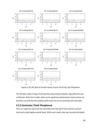
4.2.5 Conclusion (Total Phosphorus)....................................................................................110
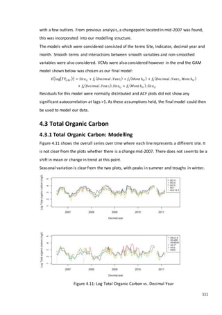
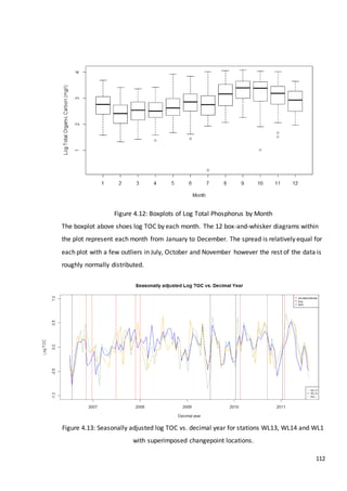
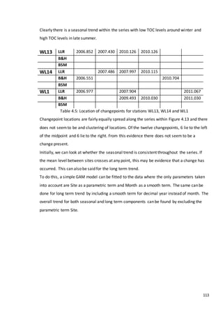
4.3 Total Organic Carbon........................................................................................................111
4.3.1 Total Organic Carbon: Modelling.................................................................................111
4.3.2 Generalised Additive Models......................................................................................115
4.3.3 Varying Coefficient Model..........................................................................................116
4.3.4 Final model................................................................................................................117
4.3.5 Conclusion (Total Organic Carbon)..............................................................................124
4.4 Nitrate.............................................................................................................................126
4.4.1 Nitrate: Modelling......................................................................................................126
4.4.2 General Additive Models............................................................................................130
4.4.3 Varying Coefficient Model..........................................................................................131
4.4.4 Final model................................................................................................................132
v
4.4.5 Conclusion (Nitrate)...................................................................................................139
4.6 Conclusions.....................................................................................................................139
5 Conclusions............................................................................................................................140
5.1 Overview.........................................................................................................................140
5.2 Results............................................................................................................................141
5.3 EMEP Results...................................................................................................................141
5.4 Whitelee results...............................................................................................................142
5.5 Discussion and limitations ................................................................................................144
Bibliography.............................................................................................................................146
vi
List of figures
Figure 1.1 Examples of interventions 5
Figure 1.2 Time seriesof logS02 at AT02 (Superimposedestimateddata) 7
Figure 1.3 Time series of log SO2 at GB02 (Superimposed estimated data) 8
Figure 1.4 Time series of log Total Phosphorus 10
Figure 1.5 Time series of log Total Organic Carbon 11
Figure 1.6 Time series of log Total Nitrate 12
Figure 2.1 Single simulated series with a change in mean at t = 30 17
Figure 2.2 Multiple simulated series with a change in mean at t = 30 20
Figure 2.3 Multiple simulated series (control) with a change in mean at t = 30 20
Figure 2.4 Map of Whitelee windfarm 23
Figure 2.5 Boxplots of before-after at each site 26
Figure 2.6 Residuals vs. Fitted values 28
Figure 2.7 Histogram of residuals 28
Figure 2.8 Boxplots of before-after at each site 29
Figure 2.9 Residuals vs. Fitted values 32
Figure 2.10 Histogram of residuals 32
Figure 2.11 Boxplots of before-after at each site 33
Figure 2.12 Residuals vs. Fitted values 36
Figure 2.13 Histogram of residuals 36
Figure 3.1 Simulation study scenarios 50
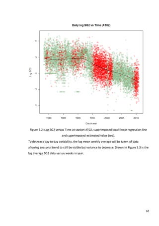
Figure 3.2 Log SO2 versus Time at station AT02, superimposed local linear
regression line and superimposed estimated value (red).
67
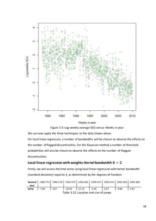
Figure 3.3 Log weekly average SO2 versus Weeks in year 68
Figure 3.4 Log weekly SO2 versus Weeks in year including location of jumps 69
Figure 3.5 Log weekly SO2 versus Weeks in year including change point locations
and non-parametric curves.
70
Figure 3.6 Log weekly SO2 versus Weeks in year including location of jumps.
Absolute value of differences between left and right smooths.
71
Figure 3.7 Log weekly average SO2 versus Weeks in year including change point 72
vii
locations and non-parametric curves.
Figure 3.8 Posterior means and Probabilities of change as calculated by Barry and
Hartigans algorithm
73
Figure 3.9 Log weekly SO2 versus weeks in year with superimposed change point
locations (p>0.90).
74
Figure 3.10 Daily log average SO2 versus weeks in year with super imposed
changepoint locations.
75
Figure 3.11 Log weekly SO2 versus weeks in year with superimposed change points 76
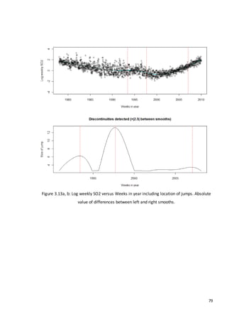
Figure 3.12 Log SO2 versus Time at station GB02, superimposed local linear
regression line and superimposed estimated values (red).
78
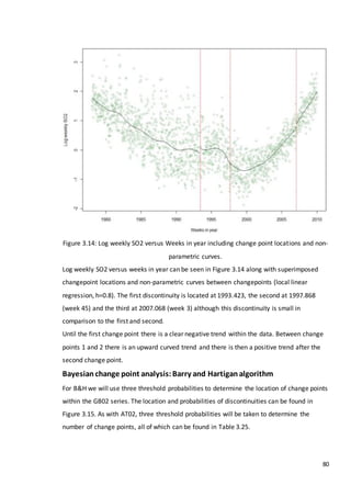
Figure 3.13 Log weekly SO2 versus Weeks in year including location of jumps.
Absolute value of differences between left and right smooths.
79
Figure 3.14 Log weekly SO2 versus Weeks in year including change point locations
and non-parametric curves.
80
Figure 3.15 Posterior means and Probabilities of change as calculated by Barry and
Hartigans algorithm
81
Figure 3.16 Log weekly SO2 versus weeks in year with superimposed change point
locations (p>0.90).
82
Figure 3.17 Log weekly SO2 vs. weeks in year with superimposed changpoint
locations
83
Figure 3.18 Log weekly SO2 versus weeks in year with superimposed change points 83
Figure 3.19 Seasonally adjusted log TP vs. decimal year for stations WL13, WL14
and WL1 with superimposed changepoint locations.
85
Figure 3.20 Seasonally adjusted log TOC vs. decimal year for stations WL13, WL14
and WL1 with superimposed changepoint locations
86
Figure 3.21 Seasonally adjusted log NO2 vs. Decimal year for stations WL13, WL14
and WL1 with superimposed changepoint locations.
87
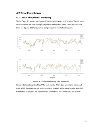
Figure 4.1 Time series of Log Total phosphorus 97
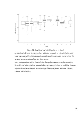
Figure 4.2 Boxplots of Log Total Phosphorus by Month 98
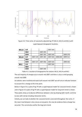
Figure 4.3 Time series of seasonally adjusted log TP (WL13, WL14 and WL1) with
superimposed changepoint locations.
99
viii
Figure 4.4 Time series of log Total Phosphorus (Superimposed seasonal
component model)
100
Figure 4.5 Time series of log Total Phosphorus (Superimposed long term trend
component model
101
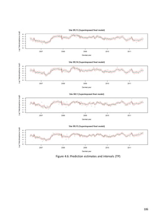
Figure 4.6 Prediction estimates and intervals (TP) 106
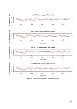
Figure 4.7 Prediction estimates and intervals (TP) 107
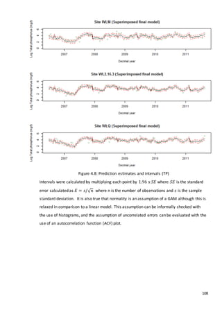
Figure 4.8 Prediction estimates and intervals (TP) 108
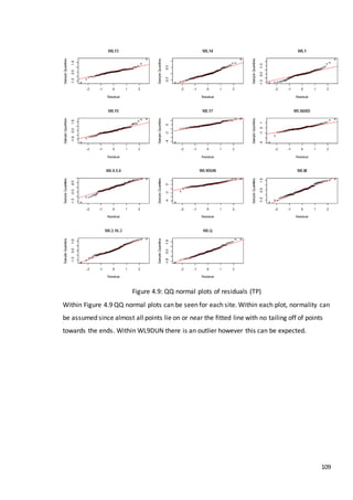
Figure 4.9 QQ normal plots of residuals (TP) 109
Figure 4.10 ACF plots of residual values at each site for log Total Phosphorus 110
Figure 4.11 Log Total Organic Carbon vs. Decimal Year 111
Figure 4.12 Boxplots of Log Total Phosphorus by Month 112
Figure 4.13 Seasonally adjusted log TOC vs. decimal year for stations WL13, WL14
and WL1 with superimposed changepoint locations.
112
Figure 4.14 Log Total Organic Carbon versus Decimal year (Superimposed long term
component model)
114
Figure 4.15 Log Total Organic Carbon versus Decimal year (Superimposed seasonal
component model)
115
Figure 4.16 Prediction estimates and intervals (TOC) 120
Figure 4.17 Prediction estimates and intervals (TOC) 121
Figure 4.18 Prediction estimates and intervals (TOC) 122
Figure 4.19 QQ normal plots at each site for log Total Organic Carbon 123
Figure 4.20 ACF plots of residual values at each site for log Total Organic Carbon 124
Figure 4.21 Log Nitrate vs. Decimal Year 126
Figure 4.22 Log Nitrate vs. Decimal Month 127
Figure 4.23 Seasonally adjusted log NO2 vs. decimal year for stations WL13, WL14
and WL1 with superimposed changepoint locations.
128
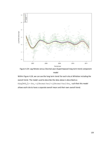
Figure 4.24 Log Nitrate versus Decimal year (Superimposed long term trend
component model
129
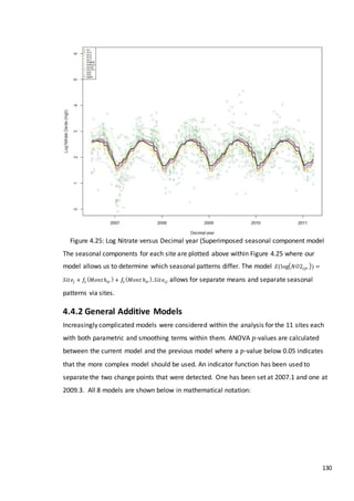
Figure 4.25 Log Nitrate versus Decimal year (Superimposed seasonal component
model
130
ix
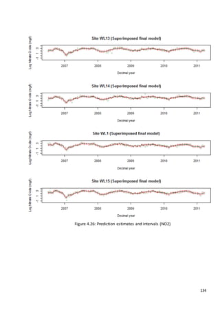
Figure 4.26 Prediction estimates and intervals (NO2) 134
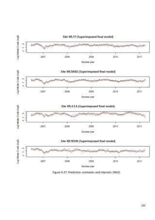
Figure 4.27 Prediction estimates and intervals (NO2) 135
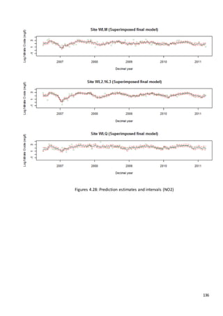
Figure 4.28 Prediction estimates and intervals (NO2) 136
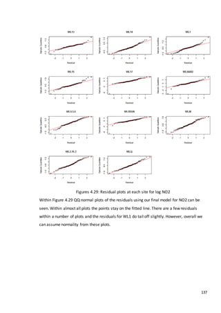
Figure 4.29 Residual plots at each site for log NO2 137
Figure 4.30 ACF plots of residual values at each site for log NO2 138
x
List of tables
Table 1.1 Locations and altitudes of EMEP stations in Europe 6
Table 1.2 Whitelee time series variables 9
Table 2.1 ANOVA table for BA design (equation 2.1) 19
Table 2.2 ANOVA table for BACI design (equation 2.2) 22
Table 2.3 Disturbance table (Provided by Helen Murray, Glasgow University) 24
Table 2.4 Table of means and mean differences 26
Table 2.5 BACI Analysis ANOVA (TP) 27
Table 2.6 Table of coefficients (TP) 28
Table 2.7 Table of means and mean differences 30
Table 2.8 BACI Analysis ANOVA (TOC) 30
Table 2.9 BACI Analysis ANOVA (TOC – reduced model) 31
Table 2.10 Table of coefficients (TOC) 31
Table 2.11 Table of means and mean differences 34
Table 2.12 BACI Analysis (NO2) 34
Table 2.13 BACI Analysis (NO2 – reduced model) 35
Table 2.14 Table of coefficients (NO2) 35
Table 2.15 Table of significant parameters 37
Table 3.1 Simulation study scenarios 50
Table 3.2 Simulation conditions 52
Table 3.3 Power and size results (LLR, Scenario 1) 53
Table 3.4 Power and size results (LLR, Scenario 2) 54
Table 3.5 Power and size results (LLR, Scenario 3) 55
Table 3.6 Power and size results (LLR, Scenario 4) 56
Table 3.7 Power and size results (LLR, Scenario 5) 57
Table 3.8 Power and size results (LLR, Scenario 6) 58
Table 3.9 Simulation conditions 59
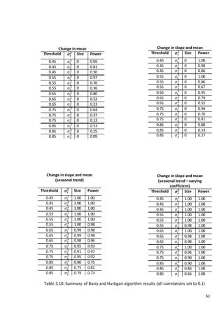
Table 3.10 Summary of Barry and Hartigan algorithm results (all correlations set
to 0.1)
62
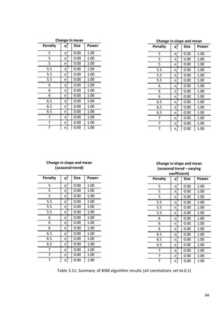
Table 3.11 Summary of BSM algorithm results (all correlations set to 0.1) 64
xi
Table 3.12 Location and size of jumps 68
Table 3.13 Location and size of jumps 71
Table 3.14 Probabilities of change with corresponding locations at various
thresholds
74
Table 3.15 Changepoints detected by BSM 75
Table 3.16 Location of change points 76
Table 3.17 Location and size of jumps 78
Table 3.18 Probabilities of change with corresponding locations at various
thresholds
81
Table 3.19 Changepoints detected by BSM 82
Table 3.20 Location of change points 84
Table 3.21 Location of changepoints for stations WL13, WL14 and WL1 86
Table 3.22 Location of changepoints for stations WL13, WL14 and WL1 87
Table 3.23 Location of changepoints for stations WL13, WL14 and WL1 89
Table 4.1 Location of changepoints for stations WL13, WL14 and WL1 99
Table 4.2 GAM models (TP) 102
Table 4.3 Varying coefficient model (TP) 103
Table 4.4 ANOVA table for final model 104
Table 4.5 Location of changepoints for stations WL13, WL14 and WL1 113
Table 4.6 GAM models (TOC) 116
Table 4.7 Final GAM model (TOC) 116
Table 4.8 Varying coefficient model (TOC) 117
Table 4.9 ANOVA table for final model (TOC) 118
Table 4.10 Comparing models with and without 𝑓(𝑀𝑜𝑛𝑡ℎ). 𝑆𝑖𝑡 𝑒𝑗 (TOC) 119
Table 4.11 Location of changepoints for stations WL13, WL14 and WL1 128
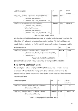
Table 4.12 GAM models (NO2) 131
Table 4.13 Final GAM model (NO2) 131
Table 4.14 Varying coefficient model (NO2) 131
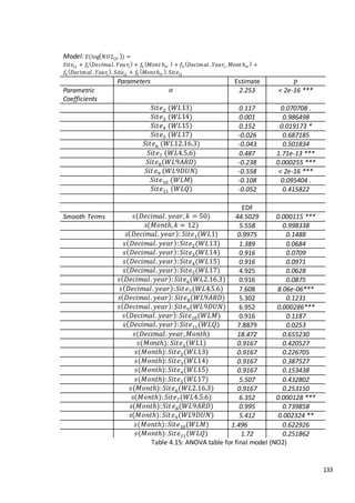
Table 4.15 ANOVA table for final model (NO2) 113
1
Chapter 1
Introduction to Changepoint Analysis and its
applications
1.1 What is Environmental Impact Assessment
Environmental Impact Assessment (EIA) is an important policy tool which is used to weigh
up evidence to assess environmental interventions, in both public and private projects.
Adopted 25 years ago, it is a procedure that ensures that the environmental implications of
decisions are taken into account before the decisions are made. Furthermore, the
complexity of the process is increased by the diversity of the disciplines involved, for
example, environmental science, social science and economics. Because of this diversity of
disciplines, the decision making procedure and final result should not be based solely on
scientific grounds but also on social viewpoints.
‘Environmental Impact Assessment’ is not strictly a statistical tool but may include some
statistical elements to provide evidence for or against environmental intervention effect on
the environment.
Created in 1985, the EIA directive has been changed three times in 1997, 2003 and 2009.
Primarily the focus of EIA is to determine whether projects will cause an environmental
impact by predicting the effects of development. The definition of an EIA as stated by the
International Association for Impact Assessment is:
2
"The process of identifying, predicting, evaluating and mitigating the biophysical, social, and
other relevant effects of development proposals prior to major decisions being taken, and
commitments made."
It also states the objectives of an EIA are as follows,
• To ensure that environmental considerations are explicitly addressed and incorporated
into the development decision making process;
• To anticipate and avoid, minimize or offset the adverse significant biophysical, social
and other relevant effects of development proposals;
• To protect the productivity and capacity of natural systems and the ecological processes
which maintain their functions; and
• To promote development that is sustainable and optimizes resource use and
management opportunities
An EIA is used to weigh up the evidence with respect to both positive and negative
consequences with regards to environmental impact. In Europe, projects must go through a
screening process to determine if an EIA is needed. Those projects already listed as an
‘Annex I’ project must have an EIA carried out, otherwise any project listed as an ‘Annex II’
project does not require an EIA (unless stated otherwise). If it is not listed as an Annex I or
Annex II, consideration is taken on deciding whether there should be an EIA at the discretion
of the state. For example, Annex I projects would include major power plants, chemical
works, waste disposal incineration and major roads. Annex II projects would include
quarries and opencast, some intensive livestock rearing, overhead transmission lines and in
some cases, wind farms. Furthermore, the location of development is a major factor in the
decision process as the environmental sensitivity is different in geographical areas.
Therefore existing land use, relative abundance of natural resources and the absorption
capacity of the natural environment must be taken into account in deciding if an EIA is
required.
If now the statistical nature of an EIA is considered, then there are issues concerning the
sampling frame over space but also over time. Data can be obtained by sampling from
various locations around the project site over time, allowing us to determine through
modelling whether the project has had any effect on the environment.
In a statistical sense, impact is determined through modelling of the observed data to infer
whether a change has taken place which can then be linked to the development.
3
Detecting a change in an environmental time series can be regarded as evidence of change
attributed to the development or project in question if the ‘experiment’ is designed
properly.
There are a number of statistical methods available to identify changes in environmental
time series. If the time at which an impact is expected to have occurred is available, Before-
After (BA) analysis is a simple way of determining whether a significant change in a variable
has been detected. When ‘control’ sites are available (sites which are relatively close to the
impact site but are not affected by the intervention) Before-After-Control-Impact (BACI)
analysis can be implemented. A literature review on BACI analysis will be carried out,
helping us to design our own analysis.
If the time of impact is not available a change point analysis can be carried out. Change
point analysis allows us to detect the time at which an impact has occurred if it is present
within a series. A literature review of various change point methods will be carried out and a
subset of the methods will be assessed. Three of these methods will be used on real life
data after conducting a simulation study to assess their performance.
Once the time of impact has been located, modelling techniques can be applied including a
dummy variable which can account for the time at which an impact has occurred. This
allows the model to ‘jump’ where an impact is present.
The approaches described above will be assessed and applied in this thesis on a variety of
environmental datasets with the purpose of locating and identify changepoints, determining
whether the change in response is significant and then modelling the data appropriately.
1.2 What is an ‘Impact’ and types of impact
The potentially impacted data series may or may not contain a shift or change in the
statistical structure of the data. If the series does contain a shift, we need to incorporate
such an effect into our models. These changes can be referred to as ‘discontinuities’ or
‘regime shifts’. The detection of discontinuities or regime shifts, are of great interest to
those who wish to model time series data efficiently. A change in parameters within a series
may affect how the series should be modelled as functions may need to be added to
account for the change. Regime shifts are cases of inhomogeneity from one relatively stable
state to another. The shifts in the series are not necessarily natural but can also be
anthropogenic. For example the introduction of a new law or the building of a new structure
4
may affect the time series variables by increasing or decreasing the mean for some given
variable for a short or long period of time, change the slope of the trend, or cause the
variable of interest to be more noisy after the change point.
The methods we wish to use depend on the design of the study. There are different ways of
determining whether an impact has occurred and its magnitude, dependent on the data we
have. It is therefore in our interests to determine:
1.) Can we detect a shift in model parameters after this intervention; do the parameters
revert to their original values after a period of time?
2.) What is the magnitude of the shift at the point of intervention?
3.) Is there evidence of trends before and after this intervention; are these trends
different?
The time series could potentially contain a combination of steps and trends. The steps may
be permanent or temporary jumps in mean values and they could be abrupt or gradual
changes. There may also be trends before and after this intervention, disrupted by the
intervention itself. These regime shifts could therefore consist of:
 A shift in the mean from 𝜇1 to some other values 𝜇2 …. . 𝜇 𝑛
 A change in regression (slope)
 The standard deviation could shift from 𝜎1 to some other value
 A combination of all 3
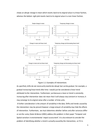
Examples of such interventions are shown below in Figure 1.1 showing the series
schematically before and after intervention with no variability or seasonal trends. Trends
that are present are assumed to be caused by the intervention, not by natural cyclic trends
in the data.
The three plots on the left of Figure 1.1 show that shifts in which the series do not decrease
back to the original value. The top left shows a simple abrupt shift in the mean value, there
is no trend in this series the mean of the series only shifts after intervention.
The plot on the left in the centre shows an abrupt shift as well as an increasing linear trend.
The plot on the bottom left also shows an abrupt shift, but a non-linear increasing trend.
The three plots on the right of Figure 1.1 show series that revert back to their original mean
value after a period of time. The top right plot shows a temporary change in mean which
increases for one time unit then reverts abruptly to its original value. The middle right plot
5
shows an abrupt change in mean which reverts back to its original value in a linear fashion,
whereas the bottom right plot reverts back to its original value in a non-linear fashion.
Figure 1.1: Examples of interventions
As specified, shifts do not necessarily need to be abrupt but can be gradual. For example, a
gradual increasing linear trend after time 𝑡 would just be considered a linear trend
attributed to the intervention. Furthermore just because a mean or trend is constantly
increasing after intervention does not mean that it will always stay constant or increase, it
may converge to its original value after a number of time units.
A further consideration is the amount of variability in the data. Shifts and trends caused by
the intervention may be present however a large amount of variability may hide the effects
of intervention. Furthermore, we must determine whether before and after variances differ
or are the same, Oaten & Bence (2001) address this problem in their paper ’Temporal and
Spatial variation in environmental impact assessment’. It is also relevant to consider the
problem of identifying whether a trend is actually caused by the intervention, or if it is
6
natural. In longer time series it is more apparent which trends are natural and which are
caused by intervention, however in short series or those that cannot be compared with
control series this may prove problematic.
1.3 Application of techniques
1.3.1 Overview
This thesis will apply a variety of change point detection methods and modelling techniques
to:
1.) European Monitoring and Evaluation Programme data on Sulphur Dioxide at various
locations in Europe.
2.) Whitelee wind farm data on Total Phosphorus, Total Organic Carbon and Nitrate
(Murray (2012)).
1.3.2 European Monitoring and Evaluation Programme (EMEP)
The EMEP measurement network monitors and evaluates concentrations of air pollutants
for over 25 years at sites situated across Europe. Many datasets are available on the EMEP
website which are freely accessible for non-commercial use including heavy metals,
Persistent Organic Pollutants (POP) particulate matter and Volatile Organic Compounds
(VOC) however within our analysis we will focus on an acidifying and eutrophying
compound, SO2 (Sulphur dioxide). There may be a presence of discontinuities in the time
series due to an international convention which limited pollutants in Europe. By assessing
this time series we can determine whether there are any statistical discontinuities using a
variety of methods. We will assess 2 datasets fromdifferent locations within the analysis,
one from Great Britain (GB02) and one from Austria (AT02). Log SO2 values will be used
within the analysis, where the analysis will be carried out on around 30 years’ worth of data.
The data which has been used can be found on the following website: http://www.emep.int/.
Locations and altitude of the 2 data sets are shown in Table 1.1.
Table 1.1: Locations and altitudes of EMEP stations in Europe.
Code Station name Latitude Longitude Altitude
AT0002R Illmitz 47 46 0 N 16 46 0 E 117
GB0002R Eskdalemuir 55 18 47 N 3 12 15 W 243
7
The sampling frequency of the data shown below in Figures 1.2 and 1.3 is daily. Much of the
data are not available due to sampling problems and therefore has to be estimated using
modelling techniques. Local linear regression with weights was chosen to estimate the
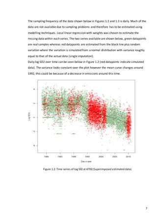
missing data within each series. The two series available are shown below, green datapoints
are real samples whereas red datapoints are estimated from the black line plus random
variation where the variation is simulated from a normal distribution with variance roughly
equal to that of the actual data (single imputation).
Daily log SO2 over time can be seen below in Figure 1.2 (red datapoints indicate simulated
data). The variance looks constant over the plot however the mean curve changes around
1992, this could be because of a decrease in emissions around this time.
Figure 1.2: Time series of log S02 at AT02 (Superimposed estimated data)
8
Figure 1.3: Time series of log SO2 at GB02 (Superimposed estimated data)
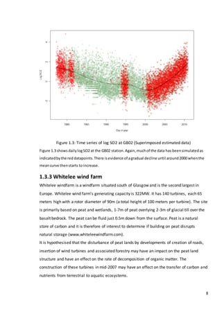
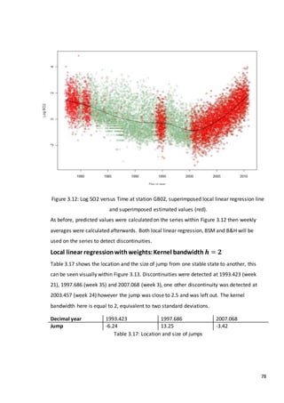
Figure 1.3 shows dailylogSO2 at the GB02 station.Again,muchof the data has beensimulatedas
indicatedbythe red datapoints.There isevidence of agradual decline until around2000 when the
meancurve thenstarts to increase.
1.3.3 Whitelee wind farm
Whitelee windfarm is a windfarm situated south of Glasgow and is the second largest in
Europe. Whitelee wind farm’s generating capacity is 322MW. It has 140 turbines, each 65
meters high with a rotor diameter of 90m (a total height of 100 meters per turbine). The site
is primarily based on peat and wetlands, 1-7m of peat overlying 2-3m of glacial till over the
basalt bedrock. The peat can be fluid just 0.5m down from the surface. Peat is a natural
store of carbon and it is therefore of interest to determine if building on peat disrupts
natural storage (www.whiteleewindfarm.com).
It is hypothesised that the disturbance of peat lands by developments of creation of roads,
insertion of wind turbines and associated forestry may have an impact on the peat land
structure and have an effect on the rate of decomposition of organic matter. The
construction of these turbines in mid-2007 may have an effect on the transfer of carbon and
nutrients from terrestrial to aquatic ecosystems.
9
Sampling is currently on-going by Anthony Waldron (The University of Edinburgh) but
previous to 2011 samples were collected and analysed by Helen Murray (University of
Glasgow).
The dataset itself consists of 8 variables across 11 sites giving around 88 time series in total
(some series are missing). A list of the 8 variables (in mg/L for all apart from CaCO3 for
alkalinity) can be found in Table 1.2.
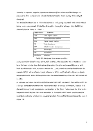
Abreviation Nutrient
TOC Total organic carbon
DOC Dissolvedorganic carbon
POC Partial organic carbon
TP Total phosphorus
SRP Soluble reactive phosphorus
NO3 Nitrate NO3
NO2 Nitrate NO2
Alkalinity Alkalinity
Table 1.2: Whitelee time series variables
Analysis will only be carried out on TP, TOC and NO2. The reason for this is that these series
have the least missing data. Estimating data within the other series would leave us with
more estimated data than real data. Stations WL13, WL14 and WL1 were chosen since it is
expected WL13 will be effected most, followed by WL14 and finally WL1. However, this is
only to determine where a changepoint lies, the overall modelling of the data will include all
11 sites.
As turbines and roads started to get built around mid-2007, we expect there will possibly be
a change point at or after this time. However the type of change is unknown, it could be a
change in mean, trend, variance or a combination of the three. Furthermore the time series
may revert to its original state after a number of years which may either be considered a
second discontinuity whether it is abrupt or gradual. A map of Whitelees sites can be seen in
Figure 2.4.
10
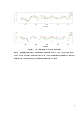
Figure 1.4 a, b: Time series of log Total Phosphorus
Figure 1.4 above shows log Total Phosphorus over time at the 11 sites, split into two plots a
and b. Around mid-2007 there does seemto be a jump in mean value however it is not clear
whether the variance or trend parameters change after this point
11
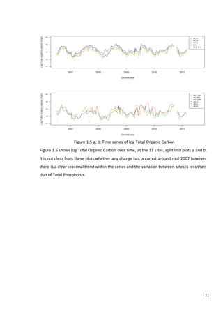
Figure 1.5 a, b: Time series of log Total Organic Carbon
Figure 1.5 shows log Total Organic Carbon over time, at the 11 sites, split into plots a and b.
It is not clear from these plots whether any change has occurred around mid-2007 however
there is a clear seasonal trend within the series and the variation between sites is less than
that of Total Phosphorus.
12
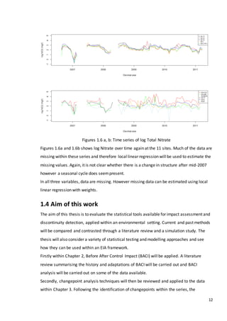
Figures 1.6 a, b: Time series of log Total Nitrate
Figures 1.6a and 1.6b shows log Nitrate over time again at the 11 sites. Much of the data are
missing within these series and therefore local linear regression will be used to estimate the
missing values. Again, it is not clear whether there is a change in structure after mid-2007
however a seasonal cycle does seempresent.
In all three variables, data are missing. However missing data can be estimated using local
linear regression with weights.
1.4 Aim of this work
The aim of this thesis is to evaluate the statistical tools available for impact assessment and
discontinuity detection, applied within an environmental setting. Current and past methods
will be compared and contrasted through a literature review and a simulation study. The
thesis will also consider a variety of statistical testing and modelling approaches and see
how they can be used within an EIA framework.
Firstly within Chapter 2, Before After Control Impact (BACI) will be applied. A literature
review summarising the history and adaptations of BACI will be carried out and BACI
analysis will be carried out on some of the data available.
Secondly, changepoint analysis techniques will then be reviewed and applied to the data
within Chapter 3. Following the identification of changepoints within the series, the
13
methods which have been evaluated previously can then be applied to EMEP data and a
number of variables from Whitelee wind farm.
In Chapter 4, once these variables are assessed for discontinuities, we can then model them
using Generalised Additive Models.
Finally, Chapter 5 will summarise the results and findings of the various approaches used
throughout the thesis.
14
Chapter 2
Before After Control Impact (BACI) design
2.1 An introduction to BACI
A very simple and easy to interpret way of determining whether an event had an ‘impact’ on
the environment is to carry out a Before After Control Impact (BACI) study.
Not only does BACI analysis allow us to evaluate whether or not an event has changed the
environment, it also allows us to estimate the magnitude of its effects.
The theory behind BACI is that we have data before, during and after the ‘event’. We also
have control sites and ‘impact sites’. These control sites are unaffected by the event as they
are either outside the area which has been affected or are under similar conditions to the
impact sites but at a different location. The control sites allow us to compare an unaffected
series with an affected one and would therefore allow us to attribute any change in the
impact site that is not observed within the control site to the ‘event’. Combined with the
availability of data before during and after the event, the design allows us to fully
understand whether the ‘event’ has made a substantial impact on the variables in question
but the time at which the ‘event’ has occurred must be known.
Adaptions of BACI have also been used. Some examples of this include studies in which data
are only available after the event, no control sites are available or only one impact site is
available with no controls.
The following section discusses the possible designs that can arise, and a literature review
discussing the different approaches that have been used.
15
2.2 Literature review on BACI analysis
The statistical model used within BACI is based entirely on the design. BACI analysis was
firstly used by Green (1979) and has since then been further adapted by a number of
authors to address various issues involving the number of control sites, number of samples
and sampling times. Green’s original design was basic, with one single sample before and
one single sample after impact at both a control site and an impact site. Bernstein & Zalinski
(1983) adapted this design to include multiple samples before and after the impact,
sampling at paired times for both control and impact sites. Oaten et al. (1986) also adopted
this design but also mentioned that to avoid coincidences with natural cycles random
sampling must be used (sometimes called BACIP, Osenberg et al. (1994)). Oaten et al. (1986)
also considered how to analyse the data using 𝑡 tests to compare means before and after
the potential impact. Further adaptations including the same design as Bernstein &
Zalinski’s but unpaired samples have been suggested.
Dealing with spatial and temporal confounding has been addressed by Bernstein & Zalinski
(1983) and Oaten et al. (1986). Beyond BACI designs developed by Underwood (1991) has
led to advances with association to human activities – designs which use multiple controls
and are analysed with asymmetrical analysis of variance because of the presence of a single
disturbed location. An example of the use of both univariate and multivariate asymmetrical
analyses can be found in Terlizzi et al. (2005) with application to Mediterranean sub tidal
sessile assemblages.
The number of impact sites and whether control sites are available will determine how the
analysis is conducted. The sites in question may all have been affected equally or a
proportion of these may have been affected by the intervention less than others, or not at
all. These sites that are not affected are called control sites, and can be used to compare
natural unaltered trends with those that have been impacted. The presence of these control
sites determine which design we must consider and which methodology can be used. Within
this section of the thesis, single series (impact) and multiple series (including only impact
sites and both impact and control sites) will be assessed and the ways in which each are
dealt with will be discussed.
16
The analyst may also want to consider the type of impact that the activity in question has.
Disturbances in the environment can be categorised into two separate areas: Pulse and
Press disturbances.
Pulses are short term episodes of disturbance which are then quickly removed, an example
of this may include oil spills which are quickly removed but for the time that the spill is
present, the impact is large. This is very different from a Press disturbance which is on-going
and constant, for example, a daily discharge of a chemical from a power plant for example.
The two types of disturbances may be very different in terms of the potential effects on the
variable in question (consult Bender et al. (1984) and Underwood (1989)) and therefore the
resulting ‘impact’ may have to be treated differently since the magnitude of effects may be
less apparent within Press disturbances and may be smoother over time.
In the following sections, each of these different settings are considered in greater detail.
2.2.1 Single series
The simplest method of impact assessment is where we have one single time series. This
time series is an impact series and is not paired with a control site, and is simply a series of
observations that contain the intervention. It is therefore a single ‘impact series’, one that
contains an impact where the time of impact is known. We have data before, during and
after this intervention hence the name Before-After design. This simple design does not
account for any temporal variability or any other causes that could affect the series
(Underwood, (1992)) as it does not have a paired control site, therefore any difference after
the intervention point 𝑡 must be attributed to the intervention. Hurlbert (1984) states that a
design which is used on single site with replicates before and after the impact are
‘pseudoreplicated’, such that any change in structure may be due to a variety of causes and
not just the ‘impact’ in question and therefore to counter this several control and impact
sites must be assessed.
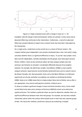
An example of this design can be seen in Figure 2.1 below, with an intervention at 𝑡 =
30 (black line is the estimated model without variation).
17
Figure 2.1: Single simulated series with a change in mean at t = 30
A problem with this design is that environmental trends are common in time series and an
observed effect may not be due to the intervention. Furthermore, a lack of an observed
effect may actually indicate an impact since a natural trend may have been interrupted by
the intervention.
For a single series, simple tests can be carried out as a means of formal analysis. The
simplest method given independent and normally distributed data is the 𝑡-test which simply
calculates whether there is a significant difference in means. To use the ‘two sample 𝑡-test’,
data must be independent, normally distributed and the groups must have equal variance
(Fisher, (1925)). 𝑡-tests can be carried out where we have unequal sample sizes and
variances, but formulas to calculate 𝑡 are denoted differently because of assumption
violation. For example, the Welch two sample 𝑡-test (Welch, (1938)) is a test used for
unequal variances. Equal variance can be formally tested with tests such as Levene's test or
the Brown–Forsythe test. Non-parametric tests such as the Mann Whitney U or Wilcoxon
signed rank can also be used when assumptions are violated as mentioned by Ruxton
(2006). Oaten et al. (1986) states that to simply conduct these tests of before versus after is
not appropriate since cyclical and long term variation is likely to occur.
To allow us to detect significant changes in mean and trend (omnibus test), a linear model
can be fitted to the data and an Analysis of Variance (ANOVA) carried out to determine
significant factors. This method is preferred where we want to determine whether there are
significant differences between more than two groups. For example, we may have multiple
intervention points within the analysis which would result in more than two separate groups
of data. The reason this method is preferred is because by conducting a multiple
18
comparisons procedure, we would need to carry out
𝑛( 𝑛−1)
2
𝑡-tests (𝑛=number of groups)
to obtain the same results.
To allow for the intervention point, an indicator variable must be set up to indicate the
changepoint. Additivity is an assumption of BACI modelling and Oaten et al. (1986) suggests
using Tukey’s test (an approach used within a two way ANOVA to assess whether the factor
variables are additively related to the expected value of the response variable) to formally
test this assumption. This problem is also discussed in Oaten (2002), Oaten (2003) and Smith
et al. (1993).
A simple model for BA design as specified in the Encyclopaedia of Environmetrics would be
as follows in equation 2.1:
𝑋𝑖𝑘 = 𝜇 + 𝛼𝑖 + 𝜏 𝑘( 𝑖) + 𝑒𝑖𝑘 (2.1)
 𝑖 is a binary indicator where 𝑖 = 𝐵(𝑏𝑒𝑓𝑜𝑟𝑒), 𝐴(𝑎𝑓𝑡𝑒𝑟)
 𝜇 is the overall mean
 𝛼𝑖 is the effect of the period
 𝜏 𝑘(𝑖) represents time within period (𝑘=1,2,3…𝑡𝐴 𝑓𝑜𝑟 𝑖 = 𝐴, 𝑘 = 1,2,3… 𝑡 𝐵 𝑓𝑜𝑟 𝑖 =
𝐵)
 𝑒𝑖𝑘 is the error term, normally distributed with constant variance.
This form could then be used within an ANOVA. From the ANOVA, the 𝑝-values in the
output will allow us to determine whether each term is significant or not. These 𝑝-values
were calculated by a series of 𝐹 tests based on mean squares. Note that the errors are
assumed to be normally distributed for this model.
It is important to note that neither 𝑡-tests nor ANOVA procedures account for temporal
variability or serial correlation in the data. This does not apply for the ANOVA if the natural
trends are taken into account within the model, however as we have stated any change at
time point 𝑡 must be attributed to the intervention as we have no paired control series in BA
design.
The standard ANOVA table for this model can be seen below within Table 2.1 where mean
squares are denoted as 𝑀𝑆 and defined as 𝑆𝑆/𝑑𝑓.
19
Source SS df F
Period: Before-After 𝑆𝑆 𝐵𝐴 1 𝑀𝑆 𝐵𝐴 /𝑀𝑆𝑡𝑖𝑚𝑒𝑠
Sampling times 𝑆𝑆𝑡𝑖𝑚𝑒𝑠 𝑡 𝐵 + 𝑡𝐴 − 2
Total 𝑆𝑆 𝑇𝑜𝑡𝑎𝑙 𝑡 𝐵 + 𝑡𝐴 − 1
Table 2.1: ANOVA table for BA design (equation 2.1)
2.2.2 Multiple series
A variation on Before-After design is to sample from a number of sites rather than observe a
single site over time. This is ultimately the same as Before-After apart from the analysis is
carried out on 𝑀 sites rather than 1 site, again each site is sampled in both periods of time
so that we have 𝑁. (𝑡 𝐵 + 𝑡𝐴 ) observations rather than 1. (𝑡 𝐵 + 𝑡𝐴 )observations. As noted in
the Encyclopedia of Environmetrics a practical problem is whether to view the sites as
replicates or subsamples – If the focus is on the extent of the impact then the sites are
selected according to a pre-set scheme and viewed as replicates. If the sites are selected at
random then they are viewed as subsamples.
There are a few differences with BA with multiple sites design compared with a BA design.
Sites are not all necessarily impact sites; a proportion of the 𝑁 sites could be control sites,
allowing us to compare the control sites with the impact sites. If this is the case, the design
is technically known as BACI (Before After Impact Control) design as we can compare
controls with impact sites. Furthermore, the fact that there is more than one site lets us
assume that the resulting change in the series is attributed to the impact rather than
coincidence since each site may have been impacted to differing extents. A problem with
this is as noted by Underwood (1992) is that similar changes at a reference site may actually
be observed by chance, meaning the impact would not be detected while using a reference
series. Underwood (1992), Underwood (1993) and Underwood (1994) adapted BACI design
further and called the analysis ‘Beyond BACI’, a design using multiple control sites to allow
researchers to distinguish natural from impact induced variability at different temporal
scales. However this design may be hard to implement due to the fact multiple controls may
not always be available. The Beyond BACI approach using multiple controls applied in an
environmental setting can be found within Musco et al. (2009), Knott et al. (2009) and
Queiroz et al. (2006) applied to sewage dumping, water pollution and oil spills respectively.
20
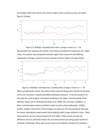
An example where two control sites and one impact series is present can be seen within
Figure 2.2 below.
Figure 2.2: Multiple simulated series with a change in mean at t = 30
Red and pink lines represent the control series whereas the black line represents the impact
series. If no control sites are present and only impact sites are present with differing
magnitudes of change, a plot of all series may look similar to Figure 2.3 shown below:
Figure 2.3: Multiple simulated series (control) with a change in mean at t = 30
When considering the control sites which will be used, the design must consider the location
of this site if variation is significantly different between locations. It must be located in an
area with the same temporal and spatial variability as the impact sites but outside of the
potential impact site as mentioned by Oaten et al. (1986). This can prove a problem, as
there is almost always natural variability in space as well as time (Underwood, (1992)).
Another problem may be that similar changes at a reference site may actually be observed
by chance, meaning the impact would not be detected while using a reference series. These
measurements are not necessarily paired in time either, if they are we can take the
difference series to ultimately remove the seasonal variation (assuming spatial variation is
constant). Furthermore these sites are not necessarily randomly selected. This introduces
21
potential analysis bias as the sites chosen as the impact sites (which are most likely chosen
for a reason) could potentially harbour systematic differences in their environmental make
up. Hurlbert (1984) criticises the analysis of designs without randomisation of impact and
control sites because of this problem and as mentioned in the previous section,
‘pseudoreplication’ can become an issue if only one control and one impact site is available
due to the fact that the two sites may have two different temporal trajectories in space and
therefore more than one control site may be needed.
In theory truly randomising impact and control sites is hardly possible in a spatial context. In
almost all cases the purpose in an EIA report is to assess the environmental impact of a man
made structure or project – it is therefore not in the interests of those conducting the
project to ‘randomly’ select an impact site as they will have probably chosen that site for a
reason.
A variety of models can now be fitted to the data, each including the indicator parameter
which identifies the point in time that an impact has been found from previous analysis.
As before, simple 𝑡-tests and non-parametric methods to determine whether population
means differ can be used. However, using these methods for BACI and especially BACI
paired designs are much better indicators of an overall effect since we can calculate t
statistics for a difference series (impact-control) rather than only on the impact series.
As stated before, we cannot determine whether there is a presence of trends with these
tests.
Linear models can again be fitted to the data and the appropriate ANOVA carried out
however if an impact site is available a difference series to remove seasonal trend can be
calculated, a parameter to deduce whether there is significant trend in the data can be
included in the model and assessed using the ANOVA. In theory by removing all seasonal
variation, all that is left in the series is the effects of interaction which can be quantified and
tested to check for significance of these trends.
The Encyclopedia of Environmetrics states that a model that can used for BACI designs is as
follows. Our response is predicted by: an overall mean, the effect of the period (before and
after), time within period, effect of location (impact of control), the interaction between
period and location and finally an error term.
A model for the BACI design as specified would be as in equation 2.2:
22
𝑋𝑖𝑗𝑘 = 𝜇 + 𝛼𝑖 + 𝜏 𝑘( 𝑖) + 𝛽𝑗 + (𝛼𝛽)𝑖𝑗 + 𝑒𝑖𝑗𝑘 (2.2)
 𝑖 is a binary indicator where 𝑖=B(before), A(after)
 𝑗 is a binary indicator where 𝑗=C(control), I(impact)
 𝜇 is the overall mean
 𝛼𝑖 is the effect of the period
 𝜏 𝑘(𝑖) represents time within period (𝑘=1,2,3…𝑡𝐴 for 𝑖=A, 𝑘=1,2,3…𝑡 𝐵 for 𝑖=B)
 𝛽𝑗 is the effect of location
 (𝛼𝛽)𝑖𝑗 is our interaction between period and location
 𝑒𝑖𝑗𝑘 is our error term, normally distributed with constant variance.
The appropriate ANOVA can then be used to determine whether there are differences in
model trajectories between impact and control sites as well as before and after
intervention. Again, p-values indicate whether each term is significant.
Within all of the above scenarios sampling times should be selected at random. This is so
that natural cycles can be accounted for which may confound the analysis if the sampling
times are fixed and far apart. In terms of including terms for seasonal patterns, harmonics
can be used relating the response variable to time (Oaten et al., (1986); Smith, (2002)). The
ANOVA table for BACI design can be seen in Table 2.2.
Source SS df F
Period: Before-After 𝑆𝑆 𝐵𝐴 1
Location: Control-
Impact
𝑆𝑆 𝐶𝐼 1
Interaction BA x CI 𝑆𝑆 𝐵𝐴𝐶𝐼 1 𝑀𝑆 𝐵𝐴𝐶𝐼 /𝑀𝑆 𝐸
Error 𝑆𝑆 𝐸 𝑁 − 4
Total 𝑆𝑆 𝑇𝑜𝑡𝑎𝑙 𝑁 − 1
Table 2.2: ANOVA table for BACI design (equation 2.2)
To summarise, if we have BA design with multiple sites we must consider:
1.) Do we have control sites, if so how many?
2.) Are the impact and control sites paired in time?
3.) Are the impact and control sites randomised?
These factors must be considered as the methods used to analyse the data series are
dependent on them. Essentially methods for different designs will be similar however the
way data are treated and the way results are interpreted will be different.
23
2.3 Application of BACI
2.3.1 Overview
Figure 2.4: Map of Whitelee windfarm
Our investigation at Whitelee can be considered as an application of BACI design. The BACI
framework here is used to evaluate changes in the determinants Total Phosphorus, Total
Organic Carbon and Nitrate following the start of deforesting in the area, the insertion of
wind turbines and inclusion of roads around Whitelee. A map of Whitelee wind farm can be
seen in Figure 2.4 which includes positions of wind turbines and the connecting roads.
Determining whether a site should be regarded as an impact or control site is not simple.
Control sites should be chosen as those which are similar to impact sites but are not likely to
be affected by intervention. We will use ‘percentage of deforested area’ around each
catchment area as an indicator of whether we can include each site as an impact or control
site. Table 2.3 below shows the percentage of deforested area at each site (note that no
data are available for sites WLM or WLQ):
24
Disturbance table: Percentage of catchment deforested
Site WL13 WL14 WL15 WL1 WL2.16.3 WL4.5.6 WL9A WL9D WL17 WL17U
% Deforested 12.2 10.3 3.5 10.7 13.2 0.8 0.5 2.3 2.0 3.9
Table 2.3: Disturbance table (Provided by Helen Murray, Glasgow University)
At each of the 11 sites, samples were taken roughly every three weeks. We will choose our
control sites as those with “Percentage of catchment deforested” less than or equal to 2%,
which means WL4.5.6, WL9A and WL17 will be chosen as our control sites.
The first analysis is based on differences between the control and impact sites paired by
sampling date. The objective is to determine if the mean difference between impact and
control sites have changed coincident with disturbance.
To obtain an initial impression, a simple before-after comparison of means will be carried
out. This allows us to determine the overall mean difference at each site and determine
whether the difference between before and after values at control sites are smaller
however this does not take into account any change in trend or seasonal pattern at the
change point.
To build our model, we need to have a term for the trend, a term to account for seasonal
pattern, a term to account for the changepoint, a term to distinguish between control and
impact sites, an interaction between the type of site and the term accounting for the
changepoint and finally an error term.
The general form of our statistical model which will be used within our BACI analysis will be
in the following form:
Response = 𝑦𝑖
Time = 𝑡𝑖
Month (Factor) = 𝑀𝑖𝑗
𝑦𝑖𝑗𝑘𝑟 = 𝜇 + 𝛽𝑡𝑖 + 𝑀𝑖𝑗 + 𝐼𝑖𝑘 + 𝐶𝐼𝑖𝑟 + 𝐼𝑖𝑘: 𝐶𝐼𝑖𝑟 + 𝑒𝑖𝑗𝑘𝑟 (2.3)
Where our sites are indicated as 𝑗 = 1, .. ,11
Our observations are indicated as 𝑖 = 1, … , 𝑛
Before or After intervention is indicated by 𝑘 = 0,1
Impact and Control sites are indicated by 𝑟 = ′
𝐼𝑚𝑝𝑎𝑐𝑡′
, ′𝐶𝑜𝑛𝑡𝑟𝑜𝑙′
𝜇 and 𝛽 are our overall mean and slope respectively.
Indicator (Factor) = 𝐼𝑖𝑘
Control/Impact(Factor) = 𝐶𝐼𝑖𝑟
Error = 𝑒𝑖𝑗𝑘𝑟
25
Our observed errors 𝑒𝑖𝑗𝑘𝑟 are assumed to be normally distributed and independent with
zero mean and constant variance.
Our parameter Indicator (𝐼𝑖𝑘)has two levels, 0 and 1 (𝑘 = 0,1). The row vector is therefore
in the following form:
𝐼𝑖𝑘 = [0,… ,0,1, … ,1]
Where the changepoint is indicated by the change in value from 0 to 1.
The parameter Control/Impact (𝐶𝐼𝑖𝑟) is a row vector with two levels 𝐼 (impact) and 𝐶
(control) ( 𝑟 = 𝐼, 𝐶)and is in the following form:
𝐶𝐼𝑖𝑟 = [𝐶, … 𝐶, 𝐼, … 𝐼]
which indicates whether a site is a control site or an impact site.
The interaction 𝐼𝑖𝑘: 𝐶𝐼𝑖𝑟 allows us to determine whether there is a difference in the change
of mean before and after the changepoint between impact and control sites.
2.3.2 Total Phosphorus
2.3.2.1 Exploratory analysis (TP)
An initial impression of the data can be obtained by comparing mean values before and
after the intervention in mid-2007.
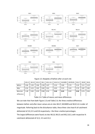
Shown below in Figure 2.3 are 11 boxplots. Within each there is one box-and-whisker for
before intervention and one after intervention. Table 2.4 also shows the mean before
intervention and the mean after at each site, as well as the absolute difference between the
two values. Absolute differences in bold are those sites that have a % deforested
of less than 2%.
26
Figure 2.5: Boxplots of before-after at each site
WL13 WL14 WL15 WL1 WL2.16.3 WL4.5.6 WL9ARD WL9DUN WL17 WLM WLQ
Before 3.06 3.39 2.86 2.94 2.87 3.35 2.84 2.74 3.24 3.11 3.19
After 4.54 4.23 3.85 3.82 3.81 4.03 3.33 3.43 3.70 3.87 3.85
Absolute
difference
1.48 0.84 0.99 0.88 0.94 0.68 0.49 0.69 0.46 0.76 0.66
Table 2.4: Table of means and mean differences
We can note that from both Figure 2.3 and Table 2.4, the three smallest differences
between before and after mean values are at sites WL17, WL9ARD and WL4.5.6 in order of
magnitude. Referring back to the disturbance table, these three sites have % of catchment
deforested of 2.0, 0.5 and 0.8 respectively – the three smallest percentages.
The largest differences were found at sites WL13, WL15 and WL2.16.3, with respective %
catchment deforested of 12.2, 3.5 and 13.2.
27
This may indicate that the sites with the smallest percentage of deforested area actually
have the smallest absolute mean difference in terms of log TP, allowing us to use them as
control sites.
2.3.2.2 BACI Analysis (TP)
The BACI analysis conducted below consisted of using a model including the terms Decimal
year, Month, Indicator (Before or After impact), Control/Impact (whether the site is a
control group or an impact group) and an interaction between Indicator and Control/Impact
as shown in equation 2.3.
Table 2.5: BACI Analysis ANOVA (TP)
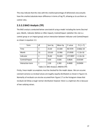
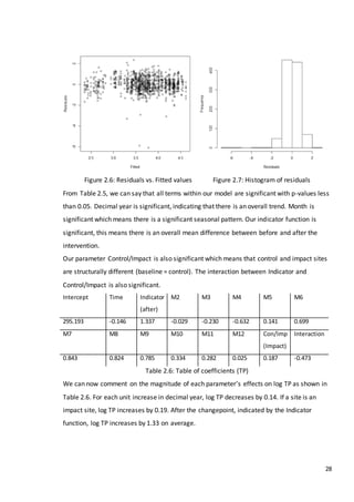
Firstly, linear model assumptions must be checked for the model above. We can assume
constant variance as residual values are roughly equally distributed as shown in Figure 2.6.
Normality of residuals can also be assumed from Figure 2.7 as the histogram shows that
residuals do follow a rough normal distribution however there is a slight tail, this is because
of two outlying values.
Term df Sum Sq Mean Sq 𝐹-value 𝑃𝑟(> 𝐹)
Time 1 21.02 21.020 40.7270 2.666e-10
Month 11 153.63 13.966 27.0590 < 2.2e-16
Indicator 1 91.82 91.824 177.9097 < 2.2e-16
Control/Impact 1 3.03 3.026 5.8626 0.01564
Interaction term 1 2.30 2.302 4.4600 0.03494
28
Figure 2.6: Residuals vs. Fitted values Figure 2.7: Histogram of residuals
From Table 2.5, we can say that all terms within our model are significant with p-values less
than 0.05. Decimal year is significant, indicating that there is an overall trend. Month is
significant which means there is a significant seasonal pattern. Our indicator function is
significant, this means there is an overall mean difference between before and after the
intervention.
Our parameter Control/Impact is also significant which means that control and impact sites
are structurally different (baseline = control). The interaction between Indicator and
Control/Impact is also significant.
Intercept Time Indicator
(after)
M2 M3 M4 M5 M6
295.193 -0.146 1.337 -0.029 -0.230 -0.632 0.141 0.699
M7 M8 M9 M10 M11 M12 Con/Imp
(Impact)
Interaction
0.843 0.824 0.785 0.334 0.282 0.025 0.187 -0.473
Table 2.6: Table of coefficients (TP)
We can now comment on the magnitude of each parameter’s effects on log TP as shown in
Table 2.6. For each unit increase in decimal year, log TP decreases by 0.14. If a site is an
impact site, log TP increases by 0.19. After the changepoint, indicated by the Indicator
function, log TP increases by 1.33 on average.
29
From Table 2.5, we can conclude that there is structural difference between control groups
and impact groups and there is also an overall mean difference before and after the
proposed impact location in time.
2.3.3 Total Organic Carbon
2.3.3.1 Exploratory analysis (TOC)
Again by comparing boxplots below and the means within Table 2.4 of before and after the
intervention at mid-2007 we can obtain an initial impression to whether changes can be
detected and whether larger changes in mean are observed within the impact sites.
Figure 2.8: Boxplots of before-after at each site
30
WL13 WL14 WL15 WL1 WL2.16.3 WL4.5.6 WL9ARD WL9DUN WL17 WLM WLQ
Before 3.04 2.94 3.15 2.88 2.95 2.63 2.49 2.09 2.30 2.66 2.67
After 3.37 3.13 3.30 3.01 3.09 2.74 2.54 2.34 2.66 2.59 2.76
Absolute
difference
0.33 0.19 0.15 0.13 0.14 0.11 0.05 0.25 0.36 0.07 0.09
Table 2.7: Table of means and mean differences
As specified, site WL4.5.6, WL9ARD and WL17 had the lowest percentage of deforested
catchment and it would be expected that these sites would be affected less than the others.
From Table 2.7, we can see that WL4.5.6, WL9ARD and WL17 had absolute differences of
0.11, 0.05 and 0.36. The absolute difference observed within WLARD is the smallest
absolute difference overall and comparatively to other sites the absolute difference
observed at WL4.5.6 is also small however the difference observed at WL17 of 0.36 is the
largest.
Overall, most absolute differences are small when compared to before and after mean
values which indicate that there may not be a large jump in the overall mean which would
make the ‘Indicator’ term within our statistical model non-significant.
From this exploratory analysis alone, it does not seem that there will be a mean difference
before and after the changepoint for this variable.
2.3.3.2 BACI Analysis (TOC)
Table 2.8: BACI Analysis ANOVA (TOC)
Of the 5 terms within the model, 3 are significant with p-values less than 0.05. These terms
are Time, Month and Control/Impact. The two terms which are not significant are the
Indicator function and the interaction between Indicator and Control/Impact.
Term df Sum Sq Mean Sq 𝐹-value 𝑃𝑟(> 𝐹)
Time 1 1.392 1.392 6.291 0.01229
Month 11 8.692 8.692 39.280 <2e-16
Indicator 1 0.221 0.221 1.002 0.3170
Control/Impact 1 19.023 19.024 85.965 <2e-16
Interaction 1 0.0961 0.096 0.434 0.5100
31
Our factor Indicator is not significant which indicates that there is no mean change in log
TOC around 2007 however our factor Control/Impact is significant indicating that there is
structural difference between control sites and impact sites.
The interaction between the indicator function and Control/Impact is not significant either,
which means there is no difference between the mean levels of log TOC for control and
impact sites.
This model can now be reduced so that only significant terms are present.
Table 2.9: BACI Analysis ANOVA (TOC – reduced model)
Within Table 2.9 is an ANOVA for the reduced model for log TOC. Only three terms are
present all with 𝑝-values less than 0.05. The interaction term was removed first and the 𝑝-
value for our indicator term reduced only slightly.
A table of coefficients for our model terms can be seen in Table 2.10.
Table 2.10: Table of coefficients (TOC)
We can now comment on the magnitude of each term’s effects on log TOC. The term Month
has 12 levels, representing each month. Therefore, log TOC varies by month. With each unit
increase in decimal year, log TOC increases by 0.05. If a site is an impact site, log TOC
decreases by 0.29 (control sites are included within the intercept).
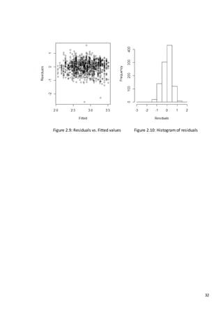
Assumptions for the model above are assessed below. Constant variance can be assumed as
the spread within the residuals vs. fitted values plot is equal and normality can be assumed
from the histogram in Figure 2.10.
Term df Sum Sq Mean Sq 𝐹-value 𝑃𝑟(> 𝐹)
Time 1 1.392 1.392 6.295 0.0122
Month 11 95.615 8.692 39.301 <2e-16
Control/Impact 1 19.024 19.024 86.014 <2e-16
Intercept Time M2 M3 M4 M5 M6 M7 M8 M9 M1O M11 M12 Con/Imp
(Impact)
-100.48 0.05 -0.3 -0.2 -0.2 -0.1 0.01 0.10 0.43 0.61 0.53 0.36 0.21 -0.29
32
Figure 2.9: Residuals vs. Fitted values Figure 2.10: Histogram of residuals
33
2.3.4 Nitrate
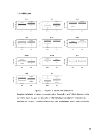
Figure 2.11: Boxplots of before-after at each site
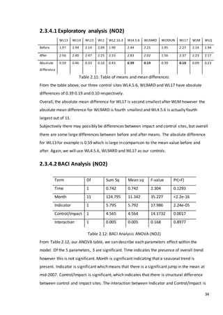
Boxplots and a table of means can be seen within Figures 2.11 and Table 2.11 respectively.
As before, mean changes can be analysed informally to give a subjective impression to
whether any changes can be found before and after and between impact and control sites.
34
2.3.4.1 Exploratory analysis (NO2)
WL13 WL14 WL15 WL1 WL2.16.3 WL4.5.6 WL9ARD WL9DUN WL17 WLM WLQ
Before 1.97 1.94 2.14 2.09 1.90 2.44 2.21 1.95 2.27 2.14 1.94
After 2.56 2.40 2.47 2.25 2.33 2.83 2.02 1.56 2.37 2.23 2.17
Absolute
difference
0.59 0.46 0.33 0.16 0.43 0.39 0.19 0.39 0.10 0.09 0.23
Table 2.11: Table of means and mean differences
From the table above, our three control sites WL4.5.6, WL9ARD and WL17 have absolute
differences of 0.39 0.19 and 0.10 respectively.
Overall, the absolute mean difference for WL17 is second smallest after WLM however the
absolute mean difference for WL9ARD is fourth smallest and WL4.5.6 is actually fourth
largest out of 11.
Subjectively there may possibly be differences between impact and control sites, but overall
there are some large differences between before and after means. The absolute difference
for WL13 for example is 0.59 which is large in comparison to the mean value before and
after. Again, we will use WL4.5.6, WL9ARD and WL17 as our controls.
2.3.4.2 BACI Analysis (NO2)
Table 2.12: BACI Analysis ANOVA (NO2)
From Table 2.12, our ANOVA table, we can describe each parameters effect within the
model. Of the 5 parameters, 3 are significant. Time indicates the presence of overall trend
however this is not significant. Month is significant indicating that a seasonal trend is
present. Indicator is significant which means that there is a significant jump in the mean at
mid-2007. Control/Impact is significant, which indicates that there is structural difference
between control and impact sites. The interaction between Indicator and Control/Impact is
Term Df Sum Sq Mean sq F-value Pr(>F)
Time 1 0.742 0.742 2.304 0.1293
Month 11 124.795 11.342 35.227 <2.2e-16
Indicator 1 5.795 5.792 17.986 2.24e-05
Control/Impact 1 4.565 4.564 14.1732 0.0017
Interaction 1 0.005 0.005 0.168 0.8977
35
not significant which means that there is no mean difference between control and impact
groups at mid-2007. This model can now be reduced so that it only contains significant
terms.
Table 2.13: BACI Analysis ANOVA (NO2 – reduced model)
Within Table 2.13 we can see the ANOVA of our final model to predict log NO2. All three
terms within this model are significant with p-values less than 0.05. A table of coefficients
for our final model can be seen in Figure 2.14.
Table 2.14: Table of coefficients (NO2)
We can interpret the model by assessing each estimate of the coefficient for each term.
As month has 12 levels, log NO2 varies with each level of this term. If a site is an Impact site,
log NO2 increases by 0.16. If we wish to estimate after the changepoint, log NO2 increases
by 0.21 on average.
Again, linear model assumptions must be checked before any analysis can take place.
Independence is again assumed by design and constant variance can be assumed from
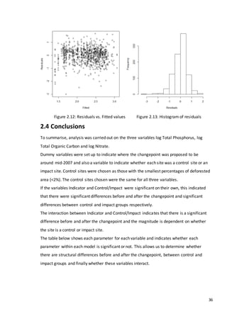
Figure 2.10 as the datapoints do not fan. Normality of residuals can also be assumed as the
histogram of residuals is bell shaped.
Term df Sum Sq Mean sq F-value Pr(>F)
Month 11 121.466 11.042 34.328 <2.2e-16
Indicator 1 9.589 9.589 29.811 6.11e-08
Control/Impact 1 4.565 4.565 14.190 0.000176
Intercept M2 M3 M4 M5 M6 M7 M8 M9 M1
O
M11 M12 Indicator
(After)
Con/Imp
(Impact)
1.39 0.11 0.26 0.46 0.69 0.96 1.08 0.93 1.10 0.84 0.73 0.51 0.21 0.16
36
Figure 2.12: Residuals vs. Fitted values Figure 2.13: Histogram of residuals
2.4 Conclusions
To summarise, analysis was carried out on the three variables log Total Phosphorus, log
Total Organic Carbon and log Nitrate.
Dummy variables were set up to indicate where the changepoint was proposed to be
around mid-2007 and also a variable to indicate whether each site was a control site or an
impact site. Control sites were chosen as those with the smallest percentages of deforested
area (<2%). The control sites chosen were the same for all three variables.
If the variables Indicator and Control/Impact were significant on their own, this indicated
that there were significant differences before and after the changepoint and significant
differences between control and impact groups respectively.
The interaction between Indicator and Control/Impact indicates that there is a significant
difference before and after the changepoint and the magnitude is dependent on whether
the site is a control or impact site.
The table below shows each parameter for each variable and indicates whether each
parameter within each model is significant or not. This allows us to determine whether
there are structural differences before and after the changepoint, between control and
impact groups and finally whether these variables interact.
37
Dec.year Month Ind Control/Impact Ind:Control/Impact
TP Yes Yes Yes Yes Yes
TOC Yes Yes No Yes No
NO2 No Yes Yes Yes No
Table 2.15: Table of significant parameters
From Table 2.15, we can see that all terms within our TP model are significant. Therefore
there is evidence of a change in mean before and after the changepoint and the magnitude
of the change depends on whether the site in question is an impact or control site. For our
TOC model, the indicator function and the two way interaction are not significant. This
means that there is no overall change in mean before and after changepoint. Our final
model for NO2 does not have a significant two way interaction or a significant overall trend.
This indicates there is no difference between impact and control sites in terms of a change
in mean at the changepoint at mid-2007.
In terms of model assumptions, all of our time series models had normality of errors. Within
our TP residuals, two were outliers however we are still able to assume normality. To
summarise, seasonal trend was present within all of our series as indicated by the
significance of month and there was also an overall structural difference between impact
and control sites within all three variables as indicated by the Control/Impact term. For each
variable, model coefficients suggested that variables were higher during the summer
months than the winter months. There was overall trend present within both TP and TOC
but not within NO2, and there was an overall mean difference within both TP and NO2 but
not TOC before and after the changepoint. Models for TP and NO2 showed that there was a
significant difference before and after the changepoint however there is no evidence to
suggest a difference in the TOC series. All three series showed significant differences
between the control and impact series.
BACI analysis only allows us to analyse whether a change occurs at a known point in time. If
this point is not known, it must be estimated. Changepoint analysis allows us to detect
changes in structure within a time series and there are many methods available to do this.
There are also problems with spatial aspects of this analysis. The control sites chosen here
were simply those which were least affected by deforestation, and were chosen after the
intervention had taken place. If control sites were chosen before the turbines had been set
38
in place and deforestation had occurred, as well as been situated far enough away not to be
affected by the intervention sites, the analysis would be much more precise. Furthermore,
temporal correlation is ignored by design which leads to the possibility of overstating
evidence for associations of interventions.
The following chapter reviews changepoint analysis and the methods that have been used
and improved within the past. Three of these techniques will be chosen and applied to a
simulation study and then applied to the real data.
39
Chapter 3
Changepoint Analysis overview and Simulation
Study
3.1 Overview of Changepoint Analysis Methods
The aim of this brief review is to assess current methodologies that are in use within EIAs. It
will mainly focus on the statistical disciplines involved in determining whether an
intervention adversely affects the environmental conditions. We will discuss methods used
by others in determining the effects of various interventions and in the process compare
and contrast the situations to which they apply these methods.
The least complicated analysis may be carried out with the use of regression techniques. For
example multiple linear regression is a linear modelling technique described by Vincent
(1996) and slightly modified by Vincent & Gullet (1999). It is used to determine where
regime shifts, if any, lie within a time series. The technique consists of the application of
four increasingly complicated linear regression models, including terms for changes in trend
and mean, for example. After the application of each model, the residuals are analysed in
order to assess fit. Consecutive significant autocorrelations in the residuals identified at low
lags indicate the poor fit of the model, and in this case the fitted model is rejected and a
different model is applied.
The use of likelihood criteria may be used to discriminate between a collection of regression
models and determine which is the best fit to the data. For example, the Bayesian/Schwarz
Information Criterion (BIC/SIC) was used by Beaulieu et al. (2010) to discriminate between
models, as is the Akaike Information Criterion (AIC) throughout the field of statistics.
However, Reeves et al. (2007) state that the BIC penalizes more heavily than the AIC and
40
tends to yield simpler models within time series. The model that minimises the AIC or BIC is
considered to be the most appropriate, taking into account both the number of parameters
and the goodness of fit by residuals. The models used can incorporate shifts in the mean,
variance, trends or combinations of these shifts.
In terms of using regression where we have access to a control series, a difference series
may be calculated and analysis may be carried out on it. Developed by Hinkley (1969), two
phase regression consisted of a model which accounted for a change point at time 𝑡. This
method has been modified by Sollow (1987), Easterling & Peterson (1995) and later by Lund
& Reeves (2002). A difference series between the impact and control series is calculated. A
simple regression model is fitted to the entire difference series and we can then obtain the
residual sum of squares denoted as 𝑅𝑆𝑆1 . We then fit two models for each data point 𝑥 𝑖:
one before and one after 𝑥 𝑖 so that we have twice as many models as data points. 𝑅𝑆𝑆2 can
then be calculated simply as the minimum of the 𝑅𝑆𝑆 values from the models we have built.
A test statistic is then calculated and if the test statistic is above a critical value, then we can
conclude there is a potential step at the data point corresponding to 𝑅𝑆𝑆2. One major
drawback mentioned by Marchant et al. (2008) is the models reliance on constant variance
of the error term, and therefore this method can only be used to determine a shift in mean
and trend but only if the variance is constant and therefore has not been affected by the
intervention. Furthermore, it is suggested that any outliers can affect the efficiency of the
least squares estimates.
The idea behind two phase regression can also be applied to non-parametric smoothing
methods where at each point within the series smooths are calculated to the left and right
of that point. If the difference in the two model trajectory’s at point 𝑥 𝑖 is large, this indicates
the presence of a discontinuity, this approach was first proposed by Hall & Titterington
(1992) and Muller (1992) with the use of kernel estimates. Many others authors that used
kernels were Speckman (1994) and Eubank & Speckman (1994) as well as many others. Local
polynomial regression methods are also widely used such as those in Gregoire & Hamrouni
(2002a) and Bowman et al. (2003).
Box & Tiao (1975) themselves developed a method to detect a change or intervention at
some time point. Intervention analysis introduced by Box & Tiao (1975) can be used to
detect and model possible trends in a set of environmental time series, specifically to
identify and model whether a statistically significant change in the time series occurs after
41
intervention. A quote from Box & Tiao’s 1975 paper states the outline of the problem
intervention analysis was intended to solve:
“Given a known intervention, is there evidence that change in the series of the kind expected
actually occurred, and, if so, what can be said of the nature and magnitude of the change?”
Intervention analysis can be used to model both abrupt and gradual effects within a series
and can accommodate both temporary and permanent changes. Examples of ‘abrupt’ and
‘gradual’ effects of intervention can be found in Timothy D Hogan’s paper on U.S fertility
rates (Hogan, (1984)). Further information on the above model can be found in Box & Tiao
(1975) or work by Abraham (1980) who subsequently extended the results for use on
multiple time series rather than a univariate case.
Other techniques have been developed such as the use of cumulative sums (CUSUM) to
determine the location of changes. Page (1954) firstly used cumulative sums to sequentially
detect discontinuities and laid the fundamental basis for its use and in 1955 he developed a
retrospective method. Since then it has been used and developed for discontinuity
detection for example by Pettitt (1980), Bagshaw & Johnson (1975) and Yashchin (1993) for
both sequential and retrospective analysis. Inclan & Tiao (1994) developed a method which
uses the cumulative sum of squares at each data point to detect a change in variance and
Rodionov (2004) developed STARS, a sequential method of using cumulative sums and t
statistics to determine the presence of regime shifts.
CUSUM is widely used within financial analysis and can be used effectively within volatility
modelling, as varying volatility can be treated as varying error. An example of CUSUM used
in this context can be seen in Inclan et al. (1999) where a generalized autoregressive
conditional heteroscedasticity (GARCH) (a model used to characterise and model observed
time series where the terms within the model are believed to have variance) framework for
errors was used and CUSUM was used to determine changes in variance. The changes in
volatility could then be attributed to world events that affect various price indexes.
Recently, many authors have used and developed Bayesian techniques to determine
whether a change has occurred. Bayesian techniques allow the user to calculate the
probability of change at each data point within the series.
Zhao et al. (2005) used Bayesian analysis with the use of MCMC to model hurricane counts
by a Poisson process where the rate parameter 𝜆 is treated as a random variable modelled
by a gamma distribution.
42
There were three hypotheses formulated: no change in the rate, single change in the rate
and double change in the rate. A hierarchical Bayesian approach was used to demonstrate
posterior probabilities of the model parameters for each hypothesis through MCMC.
Wyse et al. (2010) presented a paper which also used MCMC to perform retrospective
inference on change point models which are collapsible. Wyse rephrased the problem as a
stochastic model search over a large model space with the Bayes factors for competing
models appearing in the acceptance probabilities for the MCMC sampling scheme.
Further application of MCMC to change point detection can be seen in Antock et al. (2008)
where average year temperatures were analysed applying three models with random
coefficients. The posterior distribution of the changepoint and other parameters were
estimated from the random samples generated by the combination of the Metropolis-
Hastings algorithm and the Gibbs sampler.
de Lacy et al. (2008) explored the situation where the data could be modelled by multiple
polynomial regression and by “exploiting” Bayesian theory de Lacy proposed a method to
detect discontinuities. The proposed method consisted of applying Bayesian theory to
compute the marginal posterior distribution of the discontinuity and to detect it as
maximum a posteriori (MAP).
Beaulieu et al. (2010) presented the Bayesian Normal Homogeneity Test (BNHT). Beaulieu
states that BNHT may be applied to a series of ratios or differences between the base series
and neighbour series as proposed in Alexanderson (1986) (SNHT). Beaulieu changed the
prior probabilities of no change with 𝑝 equal to 0.01, 0.05,0.10, 0.25, 0.5, 0.75, 0.90, 0.95
and 0.99. He found: high prior probabilities of no change resulted in low false detection
rates on homogeneous series, the test had high power on a series with a single shift, small
shifts are detectable with a low prior of ‘no change’ and when the test was applied to series
with more than one shift, as well as a high probability of ‘no change’, it performed well.
Other methods for multiple change points such as reversible jump Markov chain Monte
Carlo (RJMCMC) was first proposed by Green (1995), and was used by Rotondi (2002) and
more recently by Zhao (2010).
To approximate the full posterior distributions of change point characteristics, Nam et al.
(2011) used Finite Markov Chain Imbedding in a Hidden Markov Model setting, and
accounted for parameter uncertainty via Bayesian modelling and Sequential Monte Carlo.
43
Nam states that the combination of the two is computationally efficient and does not
require estimates of the underlying state sequence.
With application to socio-economic data, Western & Kleykamp (2003) wanted to model
political relationships but by also taking into account shifts in institutions, ideas preferences
or other social conditions. They used a Gibbs sampler and also stochastically sampled from
the conditional posteriors to obtain regression coefficients in a Monte Carlo experiment.
Perreault et al. (2000) also used a Gibbs sampler along with a Markovian updating scheme
for both single change point analyses of a mean, and also of variance. A case study was
introduced to demonstrate the suitability of the Gibbs sampler in an energy inflow setting
managed by Hydro-Quebec.
In terms of application to time series data within this thesis, three methods have been
chosen. All three are used on a single series of data and each is based on different
framework.
1.) Local linear regression
2.) Binary Segmentation Method
3.) Barry and Hartigan algorithm, based on Bayesian theory
All three methods are explained in technical detail in the following section.
The remainder of this chapter will provide technical detail of the three chosen methods
then apply each to a simulation study and their performance under various conditions can
be analysed.
3.2 Applied Methods
3.2.1 Local linear regression
Bowman & Azzalini (2006) developed a method where by using normal kernel smoothing,
datum which have the largest difference between left and right model trajectories could be
used to identify the possible presence of discontinuity. He used local linear regression with
weights at each data point (potential step point 𝑡), one model that uses data from the left of
point 𝑥 𝑖 and one that uses data from the right, where the weights are taken from a normal
density function so that attention is focused only on the data lying near 𝑥 𝑖. This is done for
each data point in the whole series.
We let,
𝑦𝑖 = 𝑚( 𝑥 𝑖)+ 𝜀𝑖 (3.1)
44
Where 𝑚( 𝑥 𝑖)is a regression function of unspecified smooth shape with a finite number of
jump points and 𝜀𝑖~𝑁(0, 𝜎2
). The smoother used to estimate 𝑚( 𝑥) is local linear
regression where we need to solve
min 𝛼 ,𝛽 ∑ {𝑦𝑖 − 𝛼 − 𝛽( 𝑥 𝑖 − 𝑥)}2𝑛
𝑖=1 𝑤(𝑥 𝑖 − 𝑥; ℎ) (3.2)
and take the value of 𝛼̂ as this defines the position of the line at x. The local linear estimator
can be given by calculating ordinary least squares (OLS) with weights which gives us the
general form:
𝑚̂( 𝑥) =
1
𝑛
∑
{ 𝑠2( 𝑥;ℎ)−𝑠1( 𝑥;ℎ)( 𝑥 𝑖−𝑥)} 𝑤(𝑥 𝑖−𝑥;ℎ)𝑦𝑖
𝑠2 ( 𝑥;ℎ) 𝑠0( 𝑥;ℎ)−𝑠1 ( 𝑥;ℎ)2
𝑛
𝑖=1 (3.3)
Where 𝑤𝑖 = 𝑤(. ; ℎ) is defined by a normal distribution with mean 0 and standard deviation
h and
𝑠 𝑟( 𝑥;ℎ) = {∑(𝑥 𝑖 − 𝑥) 𝑟
𝑤( 𝑥 𝑖 − 𝑥; ℎ)}/𝑛 (3.4)
If we have extra information on each data point, this can be incorporated into the least
square function. For example, in Bowman et al. (2004) the precision of each data point in
radio carbon data is known. Bowman used
1
𝑝 𝑖
2 so that the problem now becomes:
min 𝛼 ,𝛽 ∑ {𝑦𝑖 − 𝛼 − 𝛽( 𝑥 𝑖 − 𝑥)}2𝑛
𝑖=1 𝑤(𝑥 𝑖 − 𝑥; ℎ)
1
𝑝 𝑖
2 (3.5)
which can be solved using weighted least squares to yield the linear smoother m(x). At each
point of interest x, we simply calculate local linear estimators to the left and right of x
yielding 𝑚 𝐿̂ ( 𝑥) and 𝑚 𝑅̂ ( 𝑥). If there is a jump at x then we can then calculate 𝑚̂( 𝑥−)and
𝑚̂( 𝑥+)and the basic information on the presence of a discontinuity is contained in {𝑚 𝐿̂ ( 𝑥) -
𝑚 𝑅̂ ( 𝑥)}2
. A better comparison is achieved when we standardise by the variance of the
difference such that var{𝑚 𝐿̂ ( 𝑥) - 𝑚 𝑅̂ ( 𝑥)} = 𝑣(𝑧𝑖)𝜎2
where 𝑧𝑖 = (𝑥 𝑖 + 𝑥 𝑖+1)/2 assuming
the observed 𝑥 𝑖 are arranged in an increasing order. If we have 𝑥 𝑖 = 𝑥 𝑖+1, these
observations are omitted as well as any 𝑧𝑖 which leaves less than 5 data points for the
construction of the left or right estimate (i.e if the data point is so far left or right that there
are less than 5 data points to construct a smooth we stop).
The test statistic is then:
𝑇 = ∑
{𝑚 𝐿̂ ( 𝑥) − 𝑚 𝑅̂ ( 𝑥)}2
𝑣(𝑧 𝑖)𝜎̂2
𝑔
𝑖=1 (3.6)
Where the presence of a discontinuity is expressed in the p-value 𝑃(𝑇 > 𝑇𝑜𝑏𝑠 ). The
distribution for T under the null hypothesis of the discontinuity is a shifted and scaled 𝜒2
distribution. For further details see Bowman (2006). Our null hypothesis, 𝐻0, is that no
45
discontinuities are present. Essentially the choice of h will determine the flexibility of the
model. If h is too small, the kernels will only take a small number of data points surrounding
the centre of the kernel into account which will result in a very flexible model. If h is too
large then the kernel will take too many data points into account and will not be flexible
enough. As with all methods which are based on smoothing , choosing the smoothing
parameter is always a problem. We must choose a parameter which captures enough
variability that we do not accidently detect a changepoint, but we do not want to choose a
parameter which does not detect a change because it tracks the data too closely. Because of
this, a variety of values of h will be chosen and the effects on the methods ability to detect
changepoints will be analysed.
3.2.2 Barry and Hartigan algorithm
Barry & Hartigan (2003) developed an algorithm for change point detection which assumes
that observations are independent. We let the probability of change at each point 𝑖 be given
the probability of change 𝑝𝑖. Essentially the algorithm splits the data into blocks such that
the mean is the same within each block. By applying the algorithm, we detect changepoint
between these blocks. Barry and Hartigan state that independent assumptions can be
weakened since ‘all that is required is that, given the partition and the parameters,
observations in different blocks are mutually independent’.
The prior distribution 𝜇𝑖𝑗 (the mean of the block beginning 𝑖+1 and ending 𝑗) is chosen as
𝜇𝑖𝑗~𝑁(𝜇0,
𝜎0
2
𝑗−1
) . The algorithm uses a partition 𝑝 = (𝑈1, 𝑈2, …, 𝑈 𝑛 )where 𝑈𝑖 = 1 indicates
a changepoint at position 𝑖 + 1, we initialize 𝑈𝑖 = 0 for all 𝑖 < 𝑛 .
The process starts with a Markov chain. In each step of the Markov chain, at each position 𝑖,
a value 𝑈𝑖 is drawn from the conditional distribution of 𝑈𝑖 given the data and the current
partition. Following Barry and Hartigan, we let 𝑏 denote the number of blocks obtained if
𝑈𝑖 = 0 conditional on 𝑈𝑗. The transition probability 𝑝 for the conditional probability of a
change point at the position 𝑖+1 can be obtained from the ratio:
𝑝𝑖
1−𝑝𝑖
=
𝑃( 𝑈𝑖 =1 | 𝑋,𝑈𝑗,𝑗≠𝑖)
𝑃( 𝑈𝑖=0 | 𝑋,𝑈 𝑗,𝑗≠𝑖)
(3.7)
Where 𝑊0 , 𝐵0, 𝑊1 and 𝐵1 are the within and between block sums of squares obtained when
𝑈𝑖 = 0 and 𝑈𝑖 = 1 respectively and 𝑋 is the data. The tuning parameters 𝛾 and 𝜆 allow us to
place restrictions on the priors and may take values between 0 and 1, chosen so that the
46
method is effective in situations where there are not many changes ( 𝛾 𝑠𝑚𝑎𝑙𝑙) and where
the changes that do occur are of reasonable size ( 𝜆 𝑠𝑚𝑎𝑙𝑙). After each iteration the dataset
is updated conditional on the current partition.
No null or alternative hypothesis is specified within this framework but rather a probability
of a change point being present. Therefore, we must choose cut off points for probabilities
of change, which will be discussed in the next chapter.
3.2.3 Binary Segmentation Method
Early applications of Binary Segmentation Method include Scott & Knott (1974) and Sen &
Srivastava (1975). This method uses two separate test statistics to determine if a change
point has occurred for both single and multiple changepoints.
Killick et al. (2012) developed an R package which allows users to apply BSM to time series
data.
For the single changepoint series, we consider a changepoint 𝜏1 .We will use a likelihood
ratio test statistic to determine whether there is a change in the series. The use of likelihood
ratio tests within changepoint analysis was first proposed by Hinkley (1970) and the test
statistic was firstly used to determine a change in the mean within normally distributed
data.
This method requires us to maximise the log likelihood value under both the null (no change
detected) and alternative hypotheses (change detected) where the maximum log-likelihood
value under the null hypothesis is log 𝑝(𝑦1:𝑛|𝜃̂) where 𝑝(.) is the PDF and 𝜃̂ is the MLE of
the parameters.
Under the alternative hypothesis we consider a model with changepoint at 𝜏1 where 𝜏1 can
take any value in the closed set (1,2,… . , 𝑛 − 1) then the maximum log likelihood for a given
𝜏1 is:
𝜆 = 2[𝑚𝑎𝑥𝑀𝐿( 𝜏1)− log 𝑝(𝑦1:𝑛|𝜃̂)] (3.8)
Such that we would reject 𝐻0 if 𝜆 > 𝑐 and then estimate the position of the changepoint
( 𝜏1̂ ) as the value of 𝜏1 that maximises 𝑀𝐿(𝜏1).
We can modify the single test to maximise 𝑀𝐿(𝜏1) over 𝑚 segments allowing us to
determine the location of multiple changepoints. The method requires us to minimise the
function:
∑ [𝐶(𝑦𝑚+1
𝑖=1 (𝜏𝑖−1 + 1) ∶ 𝜏𝑖 )] + 𝛽𝑓(𝑚) (3.9)
47
Here 𝐶 is a cost function for a segment and 𝛽𝑓(𝑚) is a penalty to guard against over fitting.
Using notation from the single changepoint section, 𝐶 may be taken as the negative log
likelihood and 𝛽𝑓(𝑚) may be 𝑐𝑚.
The algorithm shown below applies the single changepoint test and upon identifying a
change, iteratively implements the test statistic on the sub-segments of the data developed
by Killick et al. (2012).
Input: A set of data of the form (𝑦1, 𝑦2 , … , 𝑦 𝑛)
A test statistic 𝜆(. ) dependent on the data
An estimator of changepoint position 𝜏(. )
A rejection threshold (penalty), 𝑐
Initialise: Let 𝐶 = 𝜙 and 𝑆 = {[1, 𝑛]}
Iterate while 𝑆 ≠ 𝜙
1. Choose an element of 𝑆; denote this element as [ 𝑠, 𝑡].
2. If 𝜆( 𝑦𝑠:𝑡) < 𝑐 remove [𝑠, 𝑡] from 𝑆.
3. If 𝜆( 𝑦𝑠:𝑡) ≥ 𝑐 then;
(a) remove [ 𝑠, 𝑡] from 𝑆
(b) calculate 𝜏 = 𝜏̂( 𝑦𝑠:𝑡) + 𝑠 − 1, and add 𝜏 to 𝐶;
(c) if 𝜏 ≠ 𝑠 add [ 𝑠, 𝜏] to 𝑆
(d) if 𝜏 ≠ 𝑡 − 1 add [ 𝜏 + 1, 𝑡]to 𝑆
Output the set of changepoints recorded 𝐶
(TakenfromKillicketal.(2012))
In essence the method extends a single changepoint method to multiple changepoints by
repeating the method on varying subsets of the series iteratively:
The penalty can take any value, however Killick et al. (2012) uses 𝜆 ∗ 𝑙𝑜𝑔(𝑛) where 𝑛 is the
number of observations within the series and 𝜆 can be arbitrarily changed depending on the
expected size of the change.
3.3 Simulation study
In this section we will consider how various tests perform at detecting a discontinuity within
a time series. We wish to determine the effects of changing shape and trend in the series
48
change the chances of detecting a discontinuity when it is present within a time series, as
well as the ability to detect a discontinuity when various model parameters are changed
such as variance and serial correlation. Of the 6 cases, 3 will not include seasonal trend and
3 will include seasonal trend which reflect the application areas.
3.3.1 Statistical model
Our statistical model which we will use to assess the various approaches can be described
as:
𝑦𝑖 = 𝑓1( 𝑥 𝑖) + 𝜖𝑖 𝑤ℎ𝑒𝑟𝑒 𝑥 < 𝑐
𝑦𝑖 = 𝑓2( 𝑥 𝑖)+ 𝜖𝑖 𝑤ℎ𝑒𝑟𝑒 𝑥 ≥ 𝑐
Where the functions 𝑓1(𝑥 𝑖) and 𝑓2 (𝑥 𝑖) can be used to describe the trend of the data before
and after the change point which is denoted as 𝑐. These functions will take a variety of
forms such as straight lines and trigonometric curves to simulate seasonal trends. It is
reasonable to adopt a simple AR(1) model for the correlation structure for the error, which
can be described as:
𝜖𝑖 = 𝛼𝜖𝑖−1 + 𝑍𝑖 (3.10)
Where 𝑍𝑖 is purely random process such that 𝐸( 𝑍𝑖) = 0 and 𝑉𝑎𝑟( 𝑍𝑖) = 𝜎2
and 𝛼 is our
chosen correlation coefficient. Our error term can therefore be fully described as
𝜖~𝑁(0, 𝜎2
Σ) where Σ is our correlation matrix.
In real life situations, the correlation coefficient may have an impact on our ability to
determine if a discontinuity is present, and therefore it may be necessary to estimate this
coefficient if the test does not take autocorrelation into account. To do this, we must firstly
remove the trend that may be present within the data and perform analysis on the leftover
residual series – this can be done by using both parametric and non-parametric modelling
procedures. In this distinct case, we wish to determine the effects of changing 𝛼.
The simulation study will let us analyse the effects of changing this parameter and
determine whether we must consider estimating this coefficient before performing
subsequent analysis. In this case we did not estimate 𝛼 from any of the series, we simply
vary it to determine its effects on each tests size and power.
For each distinct case, the chosen test will be run 200 times on uniquely simulated, equally
spaced data. This allows us to determine the proportion of times the test has correctly
49
identified the discontinuity. Probability plots will be constructed to determine the areas
where the test identified where discontinuities as present.
Only one parameter will be changed at a time, leaving the rest unchanged. This allows us to
determine the effects of the change of that single parameter – and subsequently allow us to
determine which parameters are most suitable to use for our real data.
3.3.2 Size and power
The performance of the various tests can be determined by calculating the size and the
power, given various parameters of the test. Size and power can be described in terms of
type I (the odds of saying there is not a difference when there is) and type II error (the odds
of saying there is a changepoint when there is not).
Size can be calculated as the proportion of times that the test concludes that there is a
discontinuity when there is in fact not. This can be computed simply by performing the test
on a simulated series where there is no changepoint. Power can be calculated as the
proportion of times that the test concludes that there is at least one discontinuity when
there actually at least one present, and can be calculated by performing the test on series
with at least one discontinuity.
In hypothesis terms, we could say:
𝐻0: 𝑛𝑜 𝑐ℎ𝑎𝑛𝑔𝑒𝑝𝑜𝑖𝑛𝑡 𝑠𝑖𝑧𝑒 = 𝑃( 𝑟𝑒𝑗𝑒𝑐𝑡 𝐻0| 𝐻0 𝑡𝑟𝑢𝑒)
𝐻1: 𝑐ℎ𝑎𝑛𝑔𝑒𝑝𝑜𝑖𝑛𝑡 𝑝𝑜𝑤𝑒𝑟 = 𝑃(𝑟𝑒𝑗𝑒𝑐𝑡 𝐻0|𝐻1 𝑡𝑟𝑢𝑒)
3.3.3 Scenarios
We will perform the various tests on 6 distinct scenarios, listed below. The plots shown are
without random variation to show the underlying true curves.
50
Figure 3.1: Simulation study scenarios
Table 3.1: Simulation study scenarios
The error is normally distributed with constant variance, where 𝜎𝑖 was estimated from site
WL13 at Whitelee by simply fitting a local linear regression model to the series and
Model Model description
Scenario1: Change inintercept 𝑦𝑖 = 3.1 + 0.008𝑥 𝑖, 𝑖 = 1, …,50
𝑦𝑖 = 4.1 + 0.008𝑥𝑖, 𝑖 = 50, …,100
Scenario 2: Change inslope 𝑦𝑖 = 3.1 − 0.008𝑥 𝑖, 𝑖 = 1, …,50
𝑦𝑖 = 3.1 + 0.008𝑥𝑖, 𝑖 = 50, …,100
Scenario 3: Change inslope & intercept 𝑦𝑖 = 3.1 − 0.008𝑥 𝑖, 𝑖 = 1, …,50
𝑦𝑖 = 4.1 + 0.008𝑥𝑖, 𝑖 = 50, …,100
Scenario 4: Change inslope & intercept
withseasonal trend
𝑦 𝑖 = 3.6 − 0.17𝑥𝑖 − 0.1sin (
2𝜋𝑥𝑖
20
) + 0.37cos (
2𝜋𝑥𝑖
20
) , 𝑖 = 1,… ,50
𝑦 𝑖 = 4.6 + 0.17𝑥𝑖 − 0.1sin (
2𝜋𝑥𝑖
20
) + 0.37cos (
2𝜋𝑥𝑖
20
) , 𝑖 = 50,… ,100
Scenario 5: Change inslope &meanwith
seasonal trend(change inseasonal
pattern)
𝑦 𝑖 = 3.6 − 0.17𝑥𝑖 − 0.1sin (
2𝜋𝑥𝑖
20
) + 0.37cos (
2𝜋𝑥𝑖
20
) , 𝑖 = 1,… ,50
𝑦 𝑖 = 4.6 + 0.17𝑥𝑖 − 0.2sin (
2𝜋𝑥𝑖
20
) + 0.70cos (
2𝜋𝑥𝑖
20
) , 𝑖 = 50,… ,100
Scenario 6: Change inslope &meanwith
seasonal trend(change inseasonal
pattern- varyingcoefficient)
𝑦 𝑖 = 3.6 − 0.17𝑥𝑖 − 0.1sin (
2𝜋𝑥𝑖
20
) + 0.37cos (
2𝜋𝑥𝑖
20
) , 𝑖 = 1,… ,50
𝑦 𝑖 = 4.6 + 0.17𝑥𝑖 − 𝑟𝑖 sin (
2𝜋𝑥𝑖
20
) + 𝑟 𝑖 cos (
2𝜋𝑥𝑖
20
) , 𝑖 = 50,… ,100
(𝑟𝑖 increases from1 to 2, equally spaced over the 50 datapoints)
51
calculating the standard deviation from the residuals. Scenarios 1-3 are simple straight lines
with either a jump in the mean value or change in trend. Scenarios 4, 5 and 6 incorporate
trigonometric functions to represent seasonality over time, within each case 4 years’ worth
of data are represented by 4 continuous cycles.
Scenario 4 has a simple shift in the mean at the change point, with seasonal patterns which
are identical before and after this point. Scenario 5 has both a shift in the mean and also a
change in seasonal pattern, with the amplitude changing from 3 to 5 units.
Scenario 6 is the most complicated of the cases, with a varying coefficient. This coefficient
allows us to change the amplitude of the trigonometric curves where the coefficients of the
sin and cosine functions increase or decrease with time. Technically, cases 4 and 5 can be
explained by varying coefficient models, however their coefficients are constant.
3.4 Test Conditions
3.4.1 Test Conditions: Local linear regression (LLR)
Described in Section 3.1, Bowman & Azzalini (2006) developed a test based on local linear
regression with weights to determine the presence of a discontinuity. We will allow our
smoothing parameter, the bandwidth of the kernel to take a number of values – this will
allow us to determine the effect of the smoothing parameter.
Bowman’s algorithm does not take serial correlation into account when assessing the series
and by default assumes that data points are independent. The size test will therefore be
around 5% where there is no serial correlation, however if serial correlation is present this
may not be the case. A modified version of the test does allow the user to input an estimate
of the error covariance matrix into the function however since we wish to test the effects of
correlation on the test we will not use the modified version (preliminary analysis of the
Whitelee series shows no significant autocorrelation).
In real life situations, if we wish to use the modified test accounting for serial correlation, Σ
will have to be estimated, which we will call Σ̂. As mentioned previously, this can be
estimated by modelling the general trend of the data and assessing the residuals. One
problem with this method is that, especially with non-parametric smoothing techniques
where the kernel bandwidth must be chosen, the data may actually be over smoothed
resulting in a lower estimate of the correlation. The opposite is also true in that the data can
52
also be under smoothed leaving a hidden function within the data, resulting in a higher
estimate of the correlation.
From preliminary analysis we know that we do not have any significant autocorrelation, the
covariance matrix is simply an 𝐴𝑅(1)as shown below:
Σ =
[
1 𝛼 𝛼2
⋯ 𝛼 𝑛−1
𝛼 1 𝛼 ⋯ 𝛼 𝑛−2
𝛼2
𝛼 1 ⋯ 𝛼 𝑛−3
⋮ ⋮ ⋮ ⋱ ⋮
𝛼 𝑛−1
𝛼 𝑛−2
𝛼 𝑛−3
⋯ 1 ]
If the true value of 𝛼 is not known, we must obtain 𝛼̂, our estimate of the correlation, to
obtain Σ̂.
The smoothing parameter, which in this case is the kernel bandwidth of the weights must
also be chosen when carrying out this test. This is denoted as ℎ. This parameter determines
the standard deviation of the kernel, which is a normal probability distribution. This means
that points that lie close to the point of interest will have more of an influence than points
lying farther away. For scenarios 4-6, smaller values of ℎ will be used since the data has a
seasonal cycle. The smaller bandwidth allows the smoothed curve to follow the data more
closely since points that are father away, and therefore less likely to have a relationship with
the point of interest, will have less influence on the smoothed curve.
To determine each tests power we have chosen a range of bandwidths to asses. The choices
represent small moderate and large amounts of smoothing for the regression.
The simulated data will have the following characteristics:
Model and data conditions
Data spacing
Numberof simulations
Lengthof time series
Equallyspaced
100
100
Varying parameters
Error
Correlation
Kernel Bandwidth
𝜖~𝑁(0, 𝜎2Σ) , 𝜎= 0.35, 0.50, 0.65
𝜌=0.1, 0.15, 0.2
ℎ = 10,12, 14, 16,18
Table 3.2: Simulation conditions
Where within each case, various correlation coefficients, errors and smoothing parameters
will be used.
53
Scenario1: Change in mean
Correlation = 0
h 𝝈𝒊
𝟐 Size Power
10 𝜎1
2
0.07 0.74
10 𝜎2
2
0.01 0.40
10 𝜎3
2
0.10 0.31
12 𝜎1
2
0.06 0.87
12 𝜎2
2
0.01 0.48
12 𝜎3
2
0.11 0.34
14 𝜎1
2
0.04 0.94
14 𝜎2
2
0.01 0.60
14 𝜎3
2
0.11 0.39
16 𝜎1
2
0.05 0.97
16 𝜎2
2
0.03 0.62
16 𝜎3
2
0.11 0.45
18 𝜎1
2
0.05 0.99
18 𝜎2
2
0.04 0.71
18 𝜎3
2
0.09 0.48
Correlation = 0.1
h 𝝈𝒊
𝟐 Size Power
10 𝜎1
2
0.17 0.91
10 𝜎2
2
0.13 0.53
10 𝜎3
2
0.16 0.47
12 𝜎1
2
0.16 0.95
12 𝜎2
2
0.14 0.63
12 𝜎3
2
0.10 0.55
14 𝜎1
2
0.18 0.95
14 𝜎2
2
0.13 0.71
14 𝜎3
2
0.08 0.60
16 𝜎1
2
0.17 0.97
16 𝜎2
2
0.13 0.76
16 𝜎3
2
0.07 0.66
18 𝜎1
2
0.15 0.97
18 𝜎2
2
0.12 0.77
18 𝜎3
2
0.10 0.67
Correlation = 0.2
h 𝝈𝒊
𝟐 Size Power
10 𝜎1
2
0.31 0.92
10 𝜎2
2
0.36 0.78
10 𝜎3
2
0.41 0.63
12 𝜎1
2
0.36 0.95
12 𝜎2
2
0.33 0.83
12 𝜎3
2
0.38 0.68
14 𝜎1
2
0.29 1.00
14 𝜎2
2
0.32 0.85
14 𝜎3
2
0.38 0.69
16 𝜎1
2
0.29 0.99
16 𝜎2
2
0.29 0.89
16 𝜎3
2
0.34 0.72
18 𝜎1
2
0.26 0.99
18 𝜎2
2
0.27 0.88
18 𝜎3
2
0.36 0.74
Correlation = 0.15
h 𝝈𝒊
𝟐 Size Power
10 𝜎1
2
0.18 0.89
10 𝜎2
2
0.21 0.68
10 𝜎3
2
0.27 0.58
12 𝜎1
2
0.17 0.95
12 𝜎2
2
0.24 0.72
12 𝜎3
2
0.25 0.65
14 𝜎1
2
0.15 0.99
14 𝜎2
2
0.25 0.79
14 𝜎3
2
0.25 0.71
16 𝜎1
2
0.17 0.99
16 𝜎2
2
0.26 0.80
16 𝜎3
2
0.21 0.72
18 𝜎1
2
0.14 0.99
18 𝜎2
2
0.24 0.83
18 𝜎3
2
0.19 0.71
Table 3.3: Power and size results (LLR, Scenario 1)
54
Scenario2: Change in slope
Correlation = 0
h 𝝈𝒊
𝟐 Size Power
10 𝜎1
2
0.06 0.21
10 𝜎2
2
0.09 0.15
10 𝜎3
2
0.05 0.11
12 𝜎1
2
0.06 0.23
12 𝜎2
2
0.08 0.16
12 𝜎3
2
0.05 0.14
14 𝜎1
2
0.06 0.29
14 𝜎2
2
0.05 0.17
14 𝜎3
2
0.03 0.18
16 𝜎1
2
0.05 0.31
16 𝜎2
2
0.05 0.18
16 𝜎3
2
0.04 0.21
18 𝜎1
2
0.05 0.35
18 𝜎2
2
0.06 0.21
18 𝜎3
2
0.0. 0.21
Correlation = 0.1
h 𝝈𝒊
𝟐 Size Power
10 𝜎1
2
0.17 0.47
10 𝜎2
2
0.13 0.26
10 𝜎3
2
0.16 0.24
12 𝜎1
2
0.16 0.44
12 𝜎2
2
0.14 0.25
12 𝜎3
2
0.10 0.18
14 𝜎1
2
0.18 0.52
14 𝜎2
2
0.13 0.26
14 𝜎3
2
0.08 0.18
16 𝜎1
2
0.17 0.57
16 𝜎2
2
0.13 0.27
16 𝜎3
2
0.07 0.18
18 𝜎1
2
0.15 0.65
18 𝜎2
2
0.12 0.28
18 𝜎3
2
0.10 0.17
Correlation = 0.2
h 𝝈𝒊
𝟐 Size Power
10 𝜎1
2
0.31 0.54
10 𝜎2
2
0.36 0.34
10 𝜎3
2
0.41 0.47
12 𝜎1
2
0.36 0.60
12 𝜎2
2
0.33 0.39
12 𝜎3
2
0.38 0.42
14 𝜎1
2
0.29 0.65
14 𝜎2
2
0.32 0.41
14 𝜎3
2
0.38 0.40
16 𝜎1
2
0.29 0.69
16 𝜎2
2
0.29 0.40
16 𝜎3
2
0.34 0.41
18 𝜎1
2
0.26 0.71
18 𝜎2
2
0.27 0.45
18 𝜎3
2
0.36 0.37
Correlation = 0.15
h 𝝈𝒊
𝟐 Size Power
10 𝜎1
2
0.18 0.49
10 𝜎2
2
0.21 0.32
10 𝜎3
2
0.27 0.36
12 𝜎1
2
0.17 0.50
12 𝜎2
2
0.24 0.34
12 𝜎3
2
0.25 0.35
14 𝜎1
2
0.15 0.52
14 𝜎2
2
0.25 0.34
14 𝜎3
2
0.25 0.37
16 𝜎1
2
0.17 0.59
16 𝜎2
2
0.26 0.35
16 𝜎3
2
0.21 0.34
18 𝜎1
2
0.14 0.66
18 𝜎2
2
0.24 0.35
18 𝜎3
2
0.19 0.36
Table 3.4: Power and size results (LLR, Scenario 2)
55
Scenario3: Change in slope and mean
Correlation = 0
h 𝝈𝒊
𝟐 Size Power
10 𝜎1
2
0.06 0.97
10 𝜎2
2
0.09 0.81
10 𝜎3
2
0.05 0.61
12 𝜎1
2
0.06 0.98
12 𝜎2
2
0.08 0.89
12 𝜎3
2
0.05 0.77
14 𝜎1
2
0.06 1.00
14 𝜎2
2
0.05 0.93
14 𝜎3
2
0.03 0.78
16 𝜎1
2
0.05 1.00
16 𝜎2
2
0.05 0.97
16 𝜎3
2
0.04 0.81
18 𝜎1
2
0.05 1.00
18 𝜎2
2
0.06 0.97
18 𝜎3
2
0.0. 0.82
Correlation = 0.1
h 𝝈𝒊
𝟐 Size Power
10 𝜎1
2
0.17 1.00
10 𝜎2
2
0.13 0.91
10 𝜎3
2
0.16 0.67
12 𝜎1
2
0.16 1.00
12 𝜎2
2
0.14 0.98
12 𝜎3
2
0.10 0.74
14 𝜎1
2
0.18 1.00
14 𝜎2
2
0.13 0.99
14 𝜎3
2
0.08 0.79
16 𝜎1
2
0.17 1.00
16 𝜎2
2
0.13 0.99
16 𝜎3
2
0.07 0.84
18 𝜎1
2
0.15 1.00
18 𝜎2
2
0.12 0.99
18 𝜎3
2
0.10 0.87
Correlation = 0.2
h 𝝈𝒊
𝟐 Size Power
10 𝜎1
2
0.31 1.00
10 𝜎2
2
0.36 0.98
10 𝜎3
2
0.41 0.86
12 𝜎1
2
0.36 1.00
12 𝜎2
2
0.33 0.99
12 𝜎3
2
0.38 0.91
14 𝜎1
2
0.29 1.00
14 𝜎2
2
0.32 1.00
14 𝜎3
2
0.38 0.93
16 𝜎1
2
0.29 1.00
16 𝜎2
2
0.29 1.00
16 𝜎3
2
0.34 0.92
18 𝜎1
2
0.26 1.00
18 𝜎2
2
0.27 1.00
18 𝜎3
2
0.36 0.93
Correlation = 0.15
h 𝝈𝒊
𝟐 Size Power
10 𝜎1
2
0.18 1.00
10 𝜎2
2
0.21 0.96
10 𝜎3
2
0.27 0.76
12 𝜎1
2
0.17 1.00
12 𝜎2
2
0.24 0.98
12 𝜎3
2
0.25 0.82
14 𝜎1
2
0.15 1.00
14 𝜎2
2
0.25 0.99
14 𝜎3
2
0.25 0.88
16 𝜎1
2
0.17 1.00
16 𝜎2
2
0.26 0.99
16 𝜎3
2
0.21 0.89
18 𝜎1
2
0.14 1.00
18 𝜎2
2
0.24 0.99
18 𝜎3
2
0.19 0.92
Table 3.5: Power and size results (LLR, Scenario 3)
56
Scenario4: Change in slope and mean (Seasonal trend)
Correlation = 0
h 𝝈𝒊
𝟐 Size Power
2.2 𝜎1
2
0.06 0.20
2.2 𝜎2
2
0.08 0.20
2.2 𝜎3
2
0.02 0.11
2.4 𝜎1
2
0.06 0.31
2.4 𝜎2
2
0.10 0.26
2.4 𝜎3
2
0.3 0.12
2.6 𝜎1
2
0.09 0.46
2.6 𝜎2
2
0.12 0.31
2.6 𝜎3
2
0.04 0.14
2.8 𝜎1
2
0.10 0.63
2.8 𝜎2
2
0.11 0.37
2.8 𝜎3
2
0.06 0.17
3 𝜎1
2
0.13 0.76
3 𝜎2
2
0.13 0.47
3 .𝜎3
2 0.06 0.22
Correlation = 0.1
h 𝝈𝒊
𝟐 Size Power
2.2 𝜎1
2
0.11 0.53
2.2 𝜎2
2
0.15 0.32
2.2 𝜎3
2
0.19 0.31
2.4 𝜎1
2
0.13 0.63
2.4 𝜎2
2
0.14 0.38
2.4 𝜎3
2
0.20 0.31
2.6 𝜎1
2
0.17 0.74
2.6 𝜎2
2
0.19 0.45
2.6 𝜎3
2
0.26 0.32
2.8 𝜎1
2
0.28 0.89
2.8 𝜎2
2
0.23 0.58
2.8 𝜎3
2
0.29 0.38
3 𝜎1
2
0.42 0.94
3 𝜎2
2
0.25 0.70
3 𝜎3
2
0.30 0.42
Correlation = 0.2
h 𝝈𝒊
𝟐 Size Power
10 𝜎1
2
0.47 0.82
10 𝜎2
2
0.41 0.53
10 𝜎3
2
0.30 0.48
12 𝜎1
2
0.51 0.86
12 𝜎2
2
0.46 0.60
12 𝜎3
2
0.30 0.52
14 𝜎1
2
0.61 0.92
14 𝜎2
2
0.47 0.71
14 𝜎3
2
0.37 0.56
16 𝜎1
2
0.73 0.96
16 𝜎2
2
0.54 0.75
16 𝜎3
2
0.38 0.64
18 𝜎1
2
0.79 0.97
18 𝜎2
2
0.62 0.81
18 𝜎3
2
0.45 0.65
Correlation = 0.15
h 𝝈𝒊
𝟐 Size Power
10 𝜎1
2
0.32 0.69
10 𝜎2
2
0.29 0.39
10 𝜎3
2
0.31 0.38
12 𝜎1
2
0.33 0.75
12 𝜎2
2
0.29 0.45
12 𝜎3
2
0.30 0.45
14 𝜎1
2
0.38 0.84
14 𝜎2
2
0.31 0.50
14 𝜎3
2
0.31 0.48
16 𝜎1
2
0.46 0.87
16 𝜎2
2
0.38 0.65
16 𝜎3
2
0.36 0.52
18 𝜎1
2
0.57 0.96
18 𝜎2
2
0.44 0.72
18 𝜎3
2
0.45 0.59
Table 3.6: Power and size results (LLR, Scenario 4)
57
Scenario5: Change in slope and mean (Seasonal trend – increase in
amplitude)
Correlation = 0
h 𝝈𝒊
𝟐 Size Power
2.2 𝜎1
2
0.06 0.21
2.2 𝜎2
2
0.08 0.14
2.2 𝜎3
2
0.02 0.06
2.4 𝜎1
2
0.06 0.37
2.4 𝜎2
2
0.10 0.17
2.4 𝜎3
2
0.3 0.12
2.6 𝜎1
2
0.09 0.56
2.6 𝜎2
2
0.12 0.22
2.6 𝜎3
2
0.04 0.15
2.8 𝜎1
2
0.10 0.77
2.8 𝜎2
2
0.11 0.34
2.8 𝜎3
2
0.06 0.19
3 𝜎1
2
0.13 0.92
3 𝜎2
2
0.13 0.57
3 .𝜎3
2 0.06 0.26
Correlation = 0.1
h 𝝈𝒊
𝟐 Size Power
2.2 𝜎1
2
0.11 0.49
2.2 𝜎2
2
0.15 0.25
2.2 𝜎3
2
0.19 0.17
2.4 𝜎1
2
0.13 0.65
2.4 𝜎2
2
0.14 0.34
2.4 𝜎3
2
0.20 0.27
2.6 𝜎1
2
0.17 0.81
2.6 𝜎2
2
0.19 0.46
2.6 𝜎3
2
0.26 0.38
2.8 𝜎1
2
0.28 0.91
2.8 𝜎2
2
0.23 0.60
2.8 𝜎3
2
0.29 0.50
3 𝜎1
2
0.42 0.99
3 𝜎2
2
0.25 0.75
3 𝜎3
2
0.30 0.62
Correlation = 0.2
h 𝝈𝒊
𝟐 Size Power
10 𝜎1
2
0.47 0.74
10 𝜎2
2
0.41 0.65
10 𝜎3
2
0.30 0.45
12 𝜎1
2
0.51 0.86
12 𝜎2
2
0.46 0.73
12 𝜎3
2
0.30 0.50
14 𝜎1
2
0.61 0.96
14 𝜎2
2
0.47 0.82
14 𝜎3
2
0.37 0.59
16 𝜎1
2
0.73 1.00
16 𝜎2
2
0.54 0.86
16 𝜎3
2
0.38 0.68
18 𝜎1
2
0.79 1.00
18 𝜎2
2
0.62 0.95
18 𝜎3
2
0.45 0.82
Correlation = 0.15
h 𝝈𝒊
𝟐 Size Power
10 𝜎1
2
0.32 0.66
10 𝜎2
2
0.29 0.39
10 𝜎3
2
0.31 0.42
12 𝜎1
2
0.33 0.80
12 𝜎2
2
0.29 0.47
12 𝜎3
2
0.30 0.47
14 𝜎1
2
0.38 0.92
14 𝜎2
2
0.31 0.61
14 𝜎3
2
0.31 0.52
16 𝜎1
2
0.46 0.98
16 𝜎2
2
0.38 0.76
16 𝜎3
2
0.36 0.61
18 𝜎1
2
0.57 0.98
18 𝜎2
2
0.44 0.85
18 𝜎3
2
0.45 0.69
Table 3.7: Power and size results (LLR, Scenario 5)
58
Scenario6: Change in slope and mean (Seasonal trend – varying coefficient)
Correlation = 0
h 𝝈𝒊
𝟐 Size Power
2.2 𝜎1
2
0.06 0.25
2.2 𝜎2
2
0.08 0.09
2.2 𝜎3
2
0.02 0.05
2.4 𝜎1
2
0.06 0.37
2.4 𝜎2
2
0.10 0.17
2.4 𝜎3
2
0.3 0.08
2.6 𝜎1
2
0.09 0.63
2.6 𝜎2
2
0.12 0.30
2.6 𝜎3
2
0.04 0.11
2.8 𝜎1
2
0.10 0.90
2.8 𝜎2
2
0.11 0.45
2.8 𝜎3
2
0.06 0.20
3 𝜎1
2
0.13 0.99
3 𝜎2
2
0.13 0.72
3 .𝜎3
2 0.06 0.29
Correlation = 0.1
h 𝝈𝒊
𝟐 Size Power
2.2 𝜎1
2
0.11 0.47
2.2 𝜎2
2
0.15 0.28
2.2 𝜎3
2
0.19 0.24
2.4 𝜎1
2
0.13 0.70
2.4 𝜎2
2
0.14 0.40
2.4 𝜎3
2
0.20 0.39
2.6 𝜎1
2
0.17 0.92
2.6 𝜎2
2
0.19 0.60
2.6 𝜎3
2
0.26 0.39
2.8 𝜎1
2
0.28 0.99
2.8 𝜎2
2
0.23 0.75
2.8 𝜎3
2
0.29 0.52
3 𝜎1
2
0.42 1.00
3 𝜎2
2
0.25 0.91
3 𝜎3
2
0.30 0.70
Correlation = 0.2
h 𝝈𝒊
𝟐 Size Power
10 𝜎1
2
0.47 0.75
10 𝜎2
2
0.41 0.58
10 𝜎3
2
0.30 0.48
12 𝜎1
2
0.51 0.84
12 𝜎2
2
0.46 0.71
12 𝜎3
2
0.30 0.56
14 𝜎1
2
0.61 0.96
14 𝜎2
2
0.47 0.78
14 𝜎3
2
0.37 0.65
16 𝜎1
2
0.73 0.99
16 𝜎2
2
0.54 0.92
16 𝜎3
2
0.38 0.77
18 𝜎1
2
0.79 1.00
18 𝜎2
2
0.62 0.98
18 𝜎3
2
0.45 0.84
Correlation = 0.15
h 𝝈𝒊
𝟐 Size Power
10 𝜎1
2
0.32 0.61
10 𝜎2
2
0.29 0.52
10 𝜎3
2
0.31 0.38
12 𝜎1
2
0.33 0.83
12 𝜎2
2
0.29 0.62
12 𝜎3
2
0.30 0.40
14 𝜎1
2
0.38 0.96
14 𝜎2
2
0.31 0.80
14 𝜎3
2
0.31 0.53
16 𝜎1
2
0.46 0.99
16 𝜎2
2
0.38 0.88
16 𝜎3
2
0.36 0.60
18 𝜎1
2
0.57 1.00
18 𝜎2
2
0.44 0.96
18 𝜎3
2
0.45 0.75
Table 3.8: Power and size results (LLR, Scenario 6)
59
3.4.2 Test Conditions: Bayesian Change point Analysis (Barry and
Hartigan algorithm)
Described in detail in Section 3.2, Barry and Hartigan developed a method based on
Bayesian analysis to evaluate the probability of discontinuity at each data point within the
series.
The hyper parameters 𝜆 and 𝛾 are variable and can be changed and tuned assuming that we
know the number of changes and the magnitude of these changes, however, the
hyperparameters do have default values in which both are equal to 0.2 (which were found
to work well by Barry and Hartigan). Since the default value was found to work well for all
cases, we will keep them constant throughout the simulated tests.
Furthermore, the number of ‘burn-in’ (number of iterations we throw away at the start of
an MCMC run) iterations and number of iterations used in the estimation of the posterior
means are optional with a default number of burn-in iterations at 50 and default number of
iterations used for the estimation of the posterior means at 500. We will keep these
constant throughout the tests.
The conditions under which the cases were simulated are as described below:
Data spacing
Number of simulations
Length of time series
Equally spaced
100
100
Varying parameters
Error
Correlation
Threshold
𝜖~𝑁(0, 𝜎2
Σ) , 𝜎= 0.35, 0.50, 0.65
𝜌=0.1, 0.15, 0.2
ℎ = 0.45 0.55 0.65 0.75 0.85
Table 3.9: Simulation conditions
A fixed threshold value of 0.85 will be used with variable standard deviations and
correlation coefficients.
3.4.3 Test conditions: Binary Segmentation Method
For BSM, Killick et al. (2012) developed a method which uses two separate test statistics to
determine if a change point has occurred for both single and multiple changepoints.
The model structures will be the exact same as those tested by LLR & B&H with the same
variances and correlation structures.
60
We will vary the penalty variable where 𝑝𝑒𝑛 = 𝛾 ∗ log( 𝑛), allowing the parameter 𝛾 to take
the values 5, 5.5, 6, 6.5, 7. The choice of these values are arbitrary, however they allow the
test to return reasonable power while the significance lies below our threshold.
3.5 Conclusions and Results
3.5.1 Local Linear Regression
Overall this test performs very well, especially when a change in mean is present. The test
perform especially well when a seasonal trend is present as the smooths are able to account
for the pattern, however in a large number of cases the number of false positives may pose
a problem especially when correlation is present. As the correlation increases, the test is
effectively useless since as the number of false positives is so high. The tests size and power
increases rapidly as the correlation coefficient increases. For example in case 1, size is
around 0.00-0.10 with a correlation coefficient of 0 however with a correlation coefficient of
0.2 this increases to around 0.30. The presence of seasonal trend also affects the power of
the test, however, this increase in power does not mean the test performs better under
these conditions as the size also increases. Size remains under 0.10 with a correlation
coefficient of 0 however this increases with a seasonal trend to around 0.60-0.70 in some
cases.
When a change in trend is present, the power of the test is not very high. However when
both a change in trend and mean are present the power within each distinct case is higher
than the respective power for a change in mean only.
With seasonal trend, a much smaller kernel bandwidth is needed so that the smooth lines
can follow the data closer, however, the presence of this trend effects the size so much with
correlation present that to apply this to real data there must be no correlation or the
seasonal trend must be removed.
3.5.2 Barry & Hartigan algorithm
A summary of results can be found in table 3.10. Barry and Hartigan’s algorithm works very
well when seasonal trend is not present. With a simple change in mean, the power is very
high (80-90%) with standard deviation equal to 0.35. With larger standard deviation, the
power rapidly decreases, for example with a simple change in mean with a standard
61
deviation equal to 0.65 the power reduces to 0.50; however, the size always remains around
0 even with larger correlation coefficients.
With both a change in mean and change in slope and mean, as the threshold increases the
power decreases and the size stays constant at 0. For example, with both a change in mean
and slope the power reduces from 0.86 at a threshold value of 0.45 down to 0.27 at a
threshold of 0.85 (standard deviation equal to 0.65 in both cases).
With seasonal trend present, size increases under all conditions to the point that the test
cannot determine whether there is a difference between non present and present change
points as the power and size are almost identical, especially when seasonal amplitude is
increased. When seasonal trend is present and the threshold decreases, the power and size
both decrease at roughly the same rate.
To use this test effectively, seasonal trend must be removed so that only the change point is
present along with overall slope and random variation. Under these conditions, the test
works very well.
62
Table 3.10: Summary of Barry and Hartigan algorithm results (all correlations set to 0.1)
Change in slope and mean
Threshold 𝝈𝒊
𝟐 Size Power
0.45 𝜎1
2
0 1.00
0.45 𝜎2
2
0 0.98
0.45 𝜎3
2
0 0.86
0.55 𝜎1
2
0 1.00
0.55 𝜎2
2
0 0.86
0.55 𝜎3
2
0 0.67
0.65 𝜎1
2
0 0.95
0.65 𝜎2
2
0 0.79
0.65 𝜎3
2
0 0.55
0.75 𝜎1
2
0 0.94
0.75 𝜎2
2
0 0.70
0.75 𝜎3
2
0 0.41
0.85 𝜎1
2
0 0.88
0.85 𝜎2
2
0 0.53
0.85 𝜎3
2
0 0.27
Change in slope and mean
(seasonal trend)
Threshold 𝝈𝒊
𝟐 Size Power
0.45 𝜎1
2
1.00 1.00
0.45 𝜎2
2
1.00 1.00
0.45 𝜎3
2
1.00 1.00
0.55 𝜎1
2
1.00 1.00
0.55 𝜎2
2
1.00 1.00
0.55 𝜎3
2
1.00 0.98
0.65 𝜎1
2
0.99 0.98
0.65 𝜎2
2
0.99 0.98
0.65 𝜎3
2
0.98 0.96
0.75 𝜎1
2
0.95 0.93
0.75 𝜎2
2
0.91 0.97
0.75 𝜎3
2
0.95 0.92
0.85 𝜎1
2
0.80 0.75
0.85 𝜎2
2
0.75 0.81
0.85 𝜎3
2
0.79 0.73
Change in slope and mean
(seasonal trend – varying
coefficient)
Threshold 𝝈𝒊
𝟐 Size Power
0.45 𝜎1
2
1.00 1.00
0.45 𝜎2
2
1.00 1.00
0.45 𝜎3
2
1.00 1.00
0.55 𝜎1
2
1.00 1.00
0.55 𝜎2
2
1.00 1.00
0.55 𝜎3
2
0.98 1.00
0.65 𝜎1
2
1.00 1.00
0.65 𝜎2
2
0.98 1.00
0.65 𝜎3
2
0.98 1.00
0.75 𝜎1
2
1.00 1.00
0.75 𝜎2
2
0.96 1.00
0.75 𝜎3
2
0.90 1.00
0.85 𝜎1
2
0.90 1.00
0.85 𝜎2
2
0.83 1.00
0.85 𝜎3
2
0.66 1.00
Change in mean
Threshold 𝝈𝒊
𝟐 Size Power
0.45 𝜎1
2
0 0.95
0.45 𝜎2
2
0 0.81
0.45 𝜎3
2
0 0.50
0.55 𝜎1
2
0 0.97
0.55 𝜎2
2
0 0.70
0.55 𝜎3
2
0 0.36
0.65 𝜎1
2
0 0.80
0.65 𝜎2
2
0 0.52
0.65 𝜎3
2
0 0.23
0.75 𝜎1
2
0 0.64
0.75 𝜎2
2
0 0.37
0.75 𝜎3
2
0 0.13
0.85 𝜎1
2
0 0.53
0.85 𝜎2
2
0 0.25
0.85 𝜎3
2
0 0.09
63
3.5.3 Binary Segmentation Method
A summary of results for BSM with correlations set to 0.1 can be seen in Table 3.11. This
method works extremely well under all conditions. Variance, correlation and the presence
of seasonal trend do not affect the power or size in any of the cases. Size stayed at 0
throughout each simulation and power stayed at 1 in all cases apart from one. The only case
that this method did not perform well was within case 2 where no change was detected
when in fact there was a change in the slope parameter.
However, as this study simply identifies whether at least one change point has been
detected and not where the change point has been detected. Therefore there is a possibility
that the test is quite sensitive and a larger penalty parameter may need to be used.
Another problem is that the penalty parameter chosen is arbitrary. Therefore, the chances
of detecting a changepoint when it is actually present is all down to the penalty chosen. If it
is too small, it will pick up the smallest changes. If it is too large, it will not pick up even large
changes. These results are good based on the penalty chosen.
64
Table 3.11: Summary of BSM algorithm results (all correlations set to 0.1)
Change in mean
Penalty 𝝈𝒊
𝟐 Size Power
5 𝜎1
2
0.00 1.00
5 𝜎2
2
0.00 1.00
5 𝜎3
2
0.00 1.00
5.5 𝜎1
2
0.00 1.00
5.5 𝜎2
2
0.00 1.00
5.5 𝜎3
2
0.00 1.00
6 𝜎1
2
0.00 1.00
6 𝜎2
2
0.00 1.00
6 𝜎3
2
0.00 1.00
6.5 𝜎1
2
0.00 1.00
6.5 𝜎2
2
0.00 1.00
6.5 𝜎3
2
0.00 1.00
7 𝜎1
2
0.00 1.00
7 𝜎2
2
0.00 1.00
7 𝜎3
2
0.00 1.00
Change in slope and mean
(seasonal trend)
Penalty 𝝈𝒊
𝟐 Size Power
5 𝜎1
2
0.00 1.00
5 𝜎2
2
0.00 1.00
5 𝜎3
2
0.00 1.00
5.5 𝜎1
2
0.00 1.00
5.5 𝜎2
2
0.00 1.00
5.5 𝜎3
2
0.00 1.00
6 𝜎1
2
0.00 1.00
6 𝜎2
2
0.00 1.00
6 𝜎3
2
0.00 1.00
6.5 𝜎1
2
0.00 1.00
6.5 𝜎2
2
0.00 1.00
6.5 𝜎3
2
0.00 1.00
7 𝜎1
2
0.00 1.00
7 𝜎2
2
0.00 1.00
7 𝜎3
2
0.00 1.00
Change in slope and mean
(seasonal trend – varying
coefficient)
Penalty 𝝈𝒊
𝟐 Size Power
5 𝜎1
2
0.00 1.00
5 𝜎2
2
0.00 1.00
5 𝜎3
2
0.00 1.00
5.5 𝜎1
2
0.00 1.00
5.5 𝜎2
2
0.00 1.00
5.5 𝜎3
2
0.00 1.00
6 𝜎1
2
0.00 1.00
6 𝜎2
2
0.00 1.00
6 𝜎3
2
0.00 1.00
6.5 𝜎1
2
0.00 1.00
6.5 𝜎2
2
0.00 1.00
6.5 𝜎3
2
0.00 1.00
7 𝜎1
2
0.00 1.00
7 𝜎2
2
0.00 1.00
7 𝜎3
2
0.00 1.00
65
3.5.4 Summary of results
To conclude, all three tests work well under different conditions. LLR works well when a
mean change is present and is affected by both correlation and by seasonal trend, especially
when the amplitude of the trend is increased. When correlation is even slightly higher then
0, the size increases drastically. Given a series with correlation, the modified test which can
account for the correlation coefficient should be used.
B&H works extremely well when seasonal trend is not present however the size increases to
almost 1 when seasonal trend is present. It would therefore make sense to remove
seasonal trend before applying this test to the data.
BSM works very well even when seasonal trend is present. However when there is no mean
change then impacts cannot be detected. A simple change in slope parameter was not
picked up at all (case 2) and therefore this test should only be used when there is a change
in mean.
As a recommendation, B&H should not be used when seasonal trend is present. When there
is a simple change of mean within series, LLR should be used and this test also works
reasonably well when seasonal trend is present (when seasonal trend is present a smaller
kernel bandwidth should be used). BSM seems to work well under all conditions however as
noted before it is possible that the test is sensitive with the penalty parameter used in this
simulation study.
Referring back to our simulation results, it makes logical sense to remove the seasonal
pattern from each series as both LLR and B&H are seriously affected by the presence of
seasonal trend.
To remove seasonal trend, a difference series will be calculated (raw series minus the
seasonal trend modelled by harmonics) by taking the original series and taking away a
harmonic function of decimal year.
3.6 Applications
The three approaches will now be applied to real life data. Firstly, we will apply the three
tests in full to the EMEP data. The sites AT02 in Austria and GB02 in Great Britain will be
used. Each method will be applied in turn and then comparing the results by assessing if
changepoints that have been detected by each method are at a similar position.
66
A changepoint analysis will then be carried out on the Whitelee data, however the full
analysis will not be shown. A summary of results will be produced and each method can be
compared.
3.6.1 EMEP Network
The EMEP network data was taken from EMEP’s website (http://www.emep.int/) and can
be accessed publically. For both AT02 and GB02, each data point is the log weekly SO2
which was calculated by taking the log of the mean of each week. This smoothed out the
seasonal pattern within the data.
Autocorrelation was checked by producing ACF plots. No significant autocorrelation was
found within either series.
3.6.1.1 AT02: Illmitz
AT02 is a site located in Illmitz which is an area at the south eastern tip of Austria, 117
meters above sea level. Log SO2 data has been taken here and is plotted within Figure 3.2,
both with super imposed estimated values (replaced NA values) and a superimposed local
linear regression line. A small amount of variability has been added to each data point,
drawn from a normal distribution with standard deviation representative of the rest of the
series. The data are daily.
67
Figure 3.2: Log SO2 versus Time at station AT02, superimposed local linear regression line
and superimposed estimated value (red).
To decrease day to day variability, the log mean weekly average will be taken of data
allowing seasonal trend to still be visible but variance to decrease. Shown in Figure 3.3 is the
log average SO2 data versus weeks in year.
68
Figure 3.3: Log weekly average SO2 versus Weeks in year
We can now apply the three techniques to the data shown above.
For local linear regression, a number of bandwidths will be chosen to observe the effects on
the number of flagged discontinuities. For the Bayesian method a number of threshold
probabilities will also be chosen to observe the effects on the number of flagged
discontinuities.
Local linear regressionwithweights:Kernel bandwidth 𝒉 = 𝟐
Firstly, we will assess the time series using local linear regression with kernel bandwidth
(standard deviation) equal to 2, as determined by the degrees of freedom.
Table 3.12: Location and size of jumps
Decimal
year
1980.772 1989.578 1992.974 1996.082 1999.247 2003.015 2005.850 2005.885
Jump -7.00 3.07 -10.05 12.19 -5.56 2.67 -4.80 3.92
69
Where the left and right smooths leave the shaded area in Figure 3.4a, suggests the possible
presence of a discontinuity. Red vertical lines indicate where discontinuities were detected
and the precise location of these change points can be found in Table 3.12. The analysis was
on a logarithmic scale, and therefore the jumps shown within Figure 3.4 are given on a log 𝑒
Figure 3.4 a,b: Log weekly SO2 versus Weeks in year including location of jumps
scale. The magnitude each of the points can also be found in Table 3.12 but are shown
visually within Figure 3.4b (absolute magnitude has been taken and plotted). Left and right
smooths may leave the shaded confidence area for large periods of time however
discontinuities are taken to be the maximum difference between the two smooths, or the
turning points within Figure 3.4b.
Figure 3.5 helps us to visually interpret the change points and furthermore, to estimate the
individual non-parametric trend between discontinuities. Local linear regression with
70
weights was used for this however the kernel bandwidth was increased to stop the trend
picking up seasonal variation.
Figure 3.5: Log weekly SO2 versus Weeks in year including change point locations and non-
parametric curves.
Table 3.12 shows the detected change points along with the respective size of jump
between smooths. Jumps 1, 3 and 4 at 1992.974 (week 50) and 1996.082 (week 4) have the
largest jumps of 7, 10.05 and 12.19 respectively. All other jumps are less than 5 in absolute
magnitude.
Since the size of the kernel bandwidth is relatively low in this case, many discontinuities that
have been flagged may not actually be change points and seasonal variation may actually
affect the testing procedure. Increasing the size of the bandwidth ℎ, will allow our
smoothing function to fit a straighter curve and will not flag a point as a discontinuity when
in fact it is seasonal variation.
Local linear regressionwithweights:Kernel bandwidth 𝒉 = 𝟒
By increasing the kernel bandwidth such that more data points are taken into consideration
when determining the smoothing function, the number of detected change points has
71
Table 3.13: Location and size of jumps
decreased from 8 to 3. The 3 change points roughly correspond with the first three change
points within the first analysis where ℎ = 2. Figure 3.6a shows our plotted Log weekly SO2
with confidence bands and detected change points and figure 3.6b allows us to visually
Figure 3.6a, b: Log weekly SO2 versus Weeks in year including location of jumps. Absolute
value of differences between left and right smooths.
interpret the size of these changes. Table 3.13 shows the location of these jumps along with
their size. Figure 3.7 is a plot of log weekly SO2 versus weeks in year with superimposed
change point locations as well as superimposed curves between change points.
Decimal year 1980.926 1988.753 1993.530
Jump -4.75 -9.65 10.29
72
Figure 3.7: Log weekly average SO2 versus Weeks in year including change point locations
and non-parametric curves.
From Figure 3.7 we can see the three change points situated at the 48th
week in 1980, the
39th week in 1988 and the 28th
week in 1993. The mean increases from the end of the first
parametric line through to the second and then increases again from the second to the
third. After change point 3 at week 28 in 1993 the mean decreases and the non-parametric
curve shows a negative slope.
These estimated change points can now be compared with estimated change points as
detected by Barry and Hartigans algorithm.
73
Bayesianchange point analysis:Barry and Hartiganalgorithm
Figure 3.8: Posterior means and Probabilities of change as calculated by Barry and Hartigans
algorithm
Under the exact same conditions in the previous analysis, Barry and Hartigans algorithm was
used on the log weekly mean SO2 from the EMEP website. The hyper parameters 𝛾 and 𝜆
are both set to their default value of 0.2 (chosen by Barry and Hartigan). The number of
burn in iterations is set to 50 and the number of iterations after burn in is set to 500 (default
values).
Figure 3.8 allows a visual interpretation of the posterior means plotted over time as well as
the locations respective probabilities of a change point occurring at that exact location. A
number of threshold probabilities are shown below in Table 3.14 which allows us to
determine the number of change points, given an arbitrary threshold value.
74
Table 3.14: Probabilities of change with corresponding locations at various thresholds
Figure 3.9: Log weekly SO2 versus weeks in year with superimposed change point locations
(p>0.90).
It is clear from Table 3.14 that as the threshold probability drops the number of change
points increases. The largest 3 change points are located at week 12 in 2006, week 40 in
1982 and week 34 in 1984. Change points may also occurred at weeks 21 and 22 in 2005,
week 12 in 2006 and week 49 in 1993.
Binary SegmentationMethod
BSM can now be applied to the time series, which can then be compared with the two
previous methods.
Threshold CP1 CP2 CP3 CP4 CP5 CP6 CP7
0.95 Probability 0.992 0.964 0.978
Location 1982.777 1984.657 2006.240
0.90 Probability 0.992 0.964 0.900 0.912 0.914 0.978
Location 1982.777 1984.657 1993.942 2005.415 2005.434 2006.240
0.80 Probability 0.992 0.964 0.866 0.900 0912 0.914 0.978
Location 1982.777 1984.657 1984.676 1993.942 2005.415 2005.434 2006.240
75
Table 3.15: Changepoints detected by BSM
Figure 3.10: Daily log average SO2 versus weeks in year with super imposed changepoint
locations.
Three changepoints were detected while using the arbitrary penalty equal to 𝜆 ∗ 𝑙𝑜𝑔( 𝑛)
where 𝜆 is equal to 10.5. One was located at 1998.201 (week 10), one at 2005.3 (week 15)
and 1993.29 (week 15).
Binary Segmentation Method
Location
(datapoint
number)
1054.0000 1424.0000 798.0000 1221.0000 393.0000
Test statistic 635.0151 112.1629 102.8227 25.75492 23.67609
Optimal Changepoints 3
Penalty 92.74975
76
Comparing LLR, B&H and BSM:AT02
Figure 3.11: Log weekly SO2 versus weeks in year with superimposed change points
Our final figures and plots, Figure 3.11 and Table 3.16 allow us to interpret the
discontinuities detected by each method side by side. Vertical lines in black are
discontinuities indicated by Barry and Hartigans algorithm (bcp), vertical lines in red are
those as indicated by local linear regression with weights (sm.discontinuity) and blue by
binary segmentation method (bsm). Of the 11 discontinuities shown in total (two
discontinuities as indicated by B&H have been merged since they were one week apart) five
are from B&H, 3 are from local linear regression and 3 by BSM.
Table 3.16: Location of change points
LLR 1980.926 1988.753 1993.530
B&H 1982.777 1984.657 1993.942 2005.424 2006.240
BSM 1993.290 1998.201 2005.300
77
LLR estimates a change at 1980.926 (week 48) whereas B&H estimates a change 1.85 years
later at 1982.777 (week 40). This could possibly be the same point as LLR’s change point is
estimated to be the maximum difference between left and right smooths but this may not
necessarily be the exact location. Figure 3.6 indicates a difference of over |2.5| overlapping
the same region as B&H’s indication. Another very close comparison can be made in 1993.
BSM indicates a change at 1993.29 (week 15), LLR indicates a change point at 1993.530
(week 27) and B&H indicates a change 0.41 years later at 1993.942 (week 48). Again, this
could possibly be the same change point as Figure 3.10 indicates a difference in smooths
within this region, overlapping B&H’s proposed value.
A noticeable difference between methods is that B&H and BSM indicate changes at 2005
and 2006, whereas LLR does not where the kernel bandwidth is equal to 4. However where
the kernel bandwidth is equal to 2, LLR indicates changes at 2003.015 (week 1), 2005.850
(week 44) and 2005.885 (week 46) (refer to Table 3.23).
By comparing the change point indicated by B&H at 2005.424 (week 21) with the change
point as indicated by LLR (h=2) at 2005.850 (week 44) the difference is small at 0.426 years
(22 weeks). Referring to table 3.23 is it possible that this is the same point as the plot of
absolute differences overlaps B&H’s proposed value.
3.6.1.2 GB02: Eskdalemuir
Eskdalemuir is an area located within Dumfries and Galloway, Scotland near the
Scottish/English border. As within analysis for AT02, the data plotted below are log daily
SO2 where the red data is predicted data from a local linear regression model with added
normal variability representative of the rest of the data. We can therefore define the model
used to predict the data as shown below as 𝑦̂ = 𝑚( 𝑥) + 𝜀𝑖 where 𝜀𝑖~𝑁(0, 0.788).
78
Figure 3.12: Log SO2 versus Time at station GB02, superimposed local linear regression line
and superimposed estimated values (red).
As before, predicted values were calculated on the series within Figure 3.12 then weekly
averages were calculated afterwards. Both local linear regression, BSM and B&H will be
used on the series to detect discontinuities.
Local linear regressionwithweights:Kernel bandwidth 𝒉 = 𝟐
Table 3.17 shows the location and the size of jump from one stable state to another, this
can be seen visually within Figure 3.13. Discontinuities were detected at 1993.423 (week
21), 1997.686 (week 35) and 2007.068 (week 3), one other discontinuity was detected at
2003.457 (week 24) however the jump was close to 2.5 and was left out. The kernel
bandwidth here is equal to 2, equivalent to two standard deviations.
Table 3.17: Location and size of jumps
Decimal year 1993.423 1997.686 2007.068
Jump -6.24 13.25 -3.42
79
Figure 3.13a, b: Log weekly SO2 versus Weeks in year including location of jumps. Absolute
value of differences between left and right smooths.
80
Figure 3.14: Log weekly SO2 versus Weeks in year including change point locations and non-
parametric curves.
Log weekly SO2 versus weeks in year can be seen in Figure 3.14 along with superimposed
changepoint locations and non-parametric curves between changepoints (local linear
regression, h=0.8). The first discontinuity is located at 1993.423, the second at 1997.868
(week 45) and the third at 2007.068 (week 3) although this discontinuity is small in
comparison to the first and second.
Until the first change point there is a clear negative trend within the data. Between change
points 1 and 2 there is an upward curved trend and there is then a positive trend after the
second change point.
Bayesianchange point analysis:Barry and Hartiganalgorithm
For B&H we will use three threshold probabilities to determine the location of change points
within the GB02 series. The location and probabilities of discontinuities can be found in
Figure 3.15. As with AT02, three threshold probabilities will be taken to determine the
number of change points, all of which can be found in Table 3.25.
81
Figure 3.15: Posterior means and Probabilities of change as calculated by Barry and
Hartigans algorithm
The majority of large probabilities lie before the first change point as detected by local
linear regression and also around where the second change point was detected.
Table 3.18: Probabilities of change with corresponding locations at various thresholds
Threshold CP1 CP2 CP3 CP4
0.95 Probability 0.998 0.996
Location 1987.699 1991.608
0.90 Probability 0.998 0.904 0.996 0 0.924
Location 1987.699 1991.180 1991.608 1996.448
0.85 Probability 0.998 0.904 0.996 0 0.924
Location 1987.699 1991.180 1991.608 1996.448
82
Within Table 3.18 probabilities of discontinuities and their respective locations are
contained. Above 0.9, 4 locations were detected. One in 1987, two in 1991 and one in 1996.
Above 0.95 only 2 locations were detected which were in 1987 and 1991.
Figure 3.16: Log weekly SO2 versus weeks in year with superimposed change point locations
(p>0.90).
Binary SegmentationMethod
The penalty parameter is set to 3.5 ∗ log(n)here and the maximum number of
changepoints we can detect will be set to 5.
Table 3.19: Changepoints detected by BSM
Binary Segmentation Method
Location
(datapoint
number)
385.0000 1504.0000 1592.0000 992.0000 1374.0000
Test statistic 270.2248 270.2248 68.83.177 68.12605 68.1205
Optimal Changepoints 3
Penalty 92.94298
83
Figure 3.17: Log weekly SO2 vs. weeks in year with superimposed changpoint locations
Three changepoints were detected while using the penalty equal to 3.5 ∗ 𝑙𝑜𝑔( 𝑛). One was
located at the same point as located by B&H at 2007.395 (week 20), one was located slightly
later at 2007.542 (week 28) and one was located at 2009.378 (week 19).
Comparing LLR, B&H & BSM:GB02
Figure 3.18: Log weekly SO2 versus weeks in year with superimposed change points
We can now compare positions of change points flagged by LLR, B&H (p>0.9) and BSM. Of
the 12 changepoints, 4 were detected by local Barry and Hartigans algorithm, 3 were
detected by local linear regression with weights and 5 by BSM, however the discontinuity
detected in 2007 which is that very last discontinuity shown in Figure 3.18, is small.
84
Table 3.20: Location of change points
Of the change points detected by LLR and B&H, three sets are relatively close. B&H detects a
change at 1996.448 whereas LLR detects a change at 1997.686 (week 35), only just over a
year apart, however BSM detects the same change as B&H at 1996.448 (week 23). Referring
to Figure 3.13 we can see that the curves maximum is at 1997.686 (week 35) however it
does overlap 1996.448.
Another two change points which are relatively close are those situated at 1991.608 (week
31) and 1991.180 (week 9) detected by B&H and another at 1993.423 (week 21) detected by
LLR. Again, referring to Figure 3.13 the absolute value of the changes detected show that
the turning point is located at 1993.423 (week 21) however the curve does overlap the value
detected at 1991.608 (week 31). The change point detected by B&H at 1991.180 (week 9) is
also within the limits of this curve.
Three changes are relatively close around 2006, two detected by BSM lie at 2005.979 (week
50) and 2007.617 (week 32) and one detected by LLR lies at 2007.068 (week 3).
3.6.2 Whitelee Windfarm
Discussed in detail in Section 1.3.4, Whitelee windfarm is a windfarm situated south of
Glasgow and is one of the largest windfarms in Europe.
As with the EMEP analysis shown in the previous section, analysis was carried out on the
Whitelee data. Of the 11 sites, 3 sites were chosen for analysis (WL13, WL14, WL1) such that
the three changepoints techniques was applied each site. Plots of each variable can be
found with a corresponding table of changepoints.
LLR 1993.423 1997.686 2007.068
B&H 1987.699 1991.180 1991.608 1996.448
BSM 1985.148 1996.448 2003.559 2005.979 2007.617
85
3.6.2.1 Total phosphorus: Comparing WL13, WL14 and WL1
Figure 3.19: Seasonally adjusted log TP vs. decimal year for stations WL13, WL14 and WL1
with superimposed changepoint locations.
Within Figure 3.19, seasonally adjusted TP versus decimal year is plotted for the three
stations at Whitelee. We also have superimposed changepoint locations which can be found
within Table 3.21. For WL13, only one change point was detected using LLR which was
located at 2007.564 (week 29) and only one changepoint was detected using B&H located at
2007.395 (week 20), which are relatively close. Three changepoints were detected at this
station with the use of BSM at 2007.395 (week 20), 2007.542 (week 28) and 2009.378 (week
19). For WL14, 5 changepoints were found with LLR but no changepoints were found with
B&H. Four changes were detected using BSM. For WL1, one change point was found at
2007.564 (week 29) with the use of LLR, no change points were detected with B&H and one
was detected by BSM.
The most notable result is that at 2007.564 (week 29), changepoints were detected at all
three stations with the use of LLR, where the changepoint is described as the maximum
absolute difference between smooths. Furthermore, BSM detected a change very close to
this value at stations WL13 and WL14, located at 2007.542 (week 28) As this was consistent,
it is quite clear that there is a shift in the series at this point in mid-2007, at the time where
86
the new turbines were being put into place – this has had an effect on the phosphorus levels
within the area.
Another notable result is that within WL13, B&H and BSM detected changes at 2007.395
(week 20) and within WL14 LLR detected a change at 2007.385. These two values are
relatively close, and by referring to Figure 3.19 (week 20) we can deduce that this is around
the time where there is an apparent jump in the series.
To summarise, all three stations have jumps around mid-2007, around the time where new
turbines were put in place and new roads were being built. It is highly likely that the
installation of these turbines affected the phosphorus levels within the area.
Table 3.21: Location of changepoints for stations WL13, WL14 and WL1
WL13 LLR 2007.564
B&H 2007.395
BSM 2007.395 2007.542 2009.378
WL14 LLR 2007.159 2007.385 2007.564 2008.048 2009.512
B&H
BSM 2007.137 2007.466 2007.542 2009.436
WL1 LLR 2007.564
B&H
BSM 2007.446
87
3.6.2.2 Total Organic Carbon: Comparing WL13, WL14 and WL1
Figure 3.20: Seasonally adjusted log TOC vs. decimal year for stations WL13, WL14 and WL1
with superimposed changepoint locations.
Table 3.22: Location of changepoints for stations WL13, WL14 and WL1
Overall, 15 changepoints were detected over the three series. 4 were detected within WL13,
all by LLR where one was detected in 2006, one in 2007 and two in 2010. 5 (week 26) were
detected within WL14, 3 by LLR and 2 by B&H where LLR detected two in 2007 and one in
2010 and B&H detected one in 2006 and one in 2010. Finally 6 were detected within WL1
where 3 were detected by LLR and 3 by B&H, where LLR detected one in 2006, one in 2007
and one in 2011 and B&H detected one in 2009, one in 2010 and one in 2011.
Before 2008, 7 discontinuities were detected, three in 2006 where B&H detected one at
2006.551 (week 28) (WL14) and two at the end of 2006 at 2006.852 (week 44) (WL13) and
WL13 LLR 2006.852 2007.430 2010.126 2010.126
B&H
BSM
WL14 LLR 2007.486 2007.997 2010.115
B&H 2006.551 2010.704
BSM
WL1 LLR 2006.977 2007.904 2011.067
B&H 2009.493 2010.030 2011.030
BSM
88
2006.977 (WL1). Two discontinuities were detected relatively close to each other at
2007.430 (WL13) and 2007.486 (WL14) – both by LLR which may indicate a change around
this time.
Another area which has two close detected change points is at 2007.997 (week 51) (WL14)
and 2007.904 (week 47) (WL1), again indicating the possibility of change.
From 2008 to mid-way through 2009, no discontinuities were detected by either LLR or by
B&H.
At 2010.030 (WL1) and 2010.115 (WL14) changes were detected by LLR and B&H
respectively, which are relatively close. Two other close changes were detected at 2011.030
(week 1)(WL1) and 2011.067 (week 3) (WL1) by B&H and LLR respectively, which were
detected within the same series.
To conclude, there are no large clusters of changes within the series which may indicate no
changes may be present however a number of changepoints were relatively close to each
other, namely two in mid-2007, two at the end of 2007, two at the start of 2010 and two at
the start of 2010, indicating possibility of change at these times. However, no changes are
expected within 2010 and 2011 so it is probable these are due to random variation.
89
3.6.2.3 Nitrate: Comparing WL13, WL14 and WL1
Figure 3.21: Seasonally adjusted log NO2 vs. Decimal year for stations WL13, WL14 and WL1
with superimposed changepoint locations.
Overall 19 discontinuities were detected within the three time series (WL13, WL14, WL1) for
NO2, detected by the three methods LLR, B&H and BSM. Ten discontinuities were detected
by LLR, 5 by B&H and 4 by BSM. The majority of discontinuities were detected within late
2006 and mid-2007, 13 discontinuities were detected within 0.65 years around 2007.
Another cluster of discontinuities lie around mid-2009 where 4 discontinuities were
detected within series WL13 and WL14.
Table 3.23: Location of changepoints for stations WL13, WL14 and WL1
From both Figures 3.21 and Table 3.23, there is evidence to suggest that a discontinuity
occurred around 2007, and possibly another in mid-2009.
WL13 LLR 2006.854 2007.307 2009.352 2009.838
B&H 2006.929 2007.137
BSM 2007.34 2009.378
WL14 LLR 2006.852 2007.367 2007.866 2009.255
B&H 2006.929 2007.058 2009.436
BSM 2007.181
WL1 LLR 2006.852 2007.307
B&H
BSM 2007.099
90
3.7 Conclusions
The simulation study carried out allowed us to determine the strength of each of the three
tests under certain conditions. Various scenarios were constructed with differing changes in
mean, trend, seasonal patterns, correlation and variance. The size and power of each test
was then calculated by simulating data 100 times under the same unique conditions and
determining the number of times that a changepoint was detected when no change point
was present and when a changepoint was present respectively.
Once the three tests were analysed we could determine how they would perform given the
data we have. Since two of the three tests were affected by seasonal trend, seasonal trend
was removed within the Whitelee data by modelling the data with harmonic functions. The
tests were then used on the difference series (original minus trend). The EMEP data did not
have seasonal trend and therefore tests were used on the raw series.
Local linear regression was used to estimate missing values within both the EMEP and the
Whitelee series using a small kernel bandwidth allowing us to follow the trend of each series
quite closely. Random variation (Gaussian) was added onto the trend since all the data is
normally distributed. The standard deviation of the random component was calculated by
taking the standard deviation of the difference series between the estimates for local linear
regression and the raw data.
For the EMEP data, the three tests assessed sites AT02 and GB02. For AT02, 11
discontinuities were found in total. Of the 11, there were two clusters of detected
changepoints (both containing 3 changepoints each), one cluster in 1993 and one from mid-
2005 to 2006. For site GB02 there are 3 clusters of detected changepoints. One cluster is
around mid-2006 to mid-2007 (three detected within this range). Another cluster is located
in 1991 (one at 1991.18 (week 9) and one at 1991.6 (week 31)) with another changepoint
relatively close at 1993. One more cluster lies around 2006 with one change located at
2005.9 (week 46), one at 2007.1 (week 5) and another at 2007.6 (week 31).
For the Total Phosphorus data at Whitelee, two clusters of changepoints are present. One
large cluster of 12 changepoints were detected in 2007, two at the start of 2007 and ten in
the middle of 2007. Another cluster of 3 changepoints are in mid-2009.
91
Total organic carbon at Whitelee did not seemto have any clusters of changepoints but
rather a spread of changepoints throughout the series. The only two close changepoints
were located within 2011, one at 2011.067 (week 3) and one at 2011.030 (week 1).
Nitrate at Whitelee had two large clusters of detected changepoints within the series, one
around 2007 and one around mid-2009. 13 detected changepoints were found around 2007,
5 late 2006 and 8 early 2007. 4 changepoints were located around mid-2009 and a further 1
in late 2009.
To conclude, for the EMEP data detected changepoints were relatively spread out with a
few clusters of detected changes in the series. For the Whitelee series, there were clusters
of changepoints in both the Total Phosphorus series and the Nitrate series, but not for the
Total Organic Carbon series, however from preliminary analysis this was to be expected.
This similarity in the location of the changepoints indicates that it is likely that the detected
changes at these clusters are very likely to truly be changepoints rather than the methods
variation.
92
Chapter 4
Modelling the trends and changes in
determinands at Whitelee
4.1 Introduction
The purpose of this chapter is to model our time series data with the use of a number of
modelling techniques.
Information gained from previous chapters can be used within our modelling process to
help build our models, making them a better fit to the data. The use of an 𝑖𝑛𝑑𝑖𝑐𝑎𝑡𝑜𝑟
function for example to indicate a changepoint, used within Chapter 2 for our BACI
modelling and adjusted within Chapter 3 using changepoint analysis, can be used to help
our models move more freely.
Models built within this chapter will be compared and contrasted with the use of various
criteria, allowing us to adapt and refine then.
These models will be built logically with the use of this previously gained information,
including parameters that we know are likely to add value to our models, rather than
building from the ground up.
Several modelling techniques may be considered while analysing the various time series of
the three variables TP, TOC and NO2. One of the techniques which will be considered is
GAMs. GAMs are made of parametric terms and non-parametric smoothing terms. This
allows for parametric characteristics with the benefit of smooth terms – GAMs are flexible
and effective for conducting nonlinear regression.
93
4.1.1 Generalised Additive Models
For generalised additive models, we assume 𝜇𝑖 = 𝐸( 𝑌𝑖) and 𝑌𝑖~ some exponential family
distribution (in this case, they are normally distributed). 𝑌𝑖 can be regarded as our response
variable, 𝑋 is our model matrix for any parametric components of our model and 𝛽 the
corresponding parameter vector. 𝑓𝑖 𝑠 are regarded as our smooth functions of covariates 𝑥 𝑘.
Various smoothing functions can be used and the basis can be chosen, where the 𝑏𝑎𝑠𝑖𝑠 is
defined as the type of smoothing function we use. Within our analysis, we will use
regression splines and cubic regression splines, the latter when representing seasonal
variation.
Representing a smooth function via regression splines requires that 𝑓 be represented in
such a way that it becomes a linear model, whereas representing a smooth via a cubic spline
is made up of sections of cubic polynomial to make a curve. These sections that the sections
meet are called 𝑘𝑛𝑜𝑡𝑠 and must be chosen, typically evenly spaced through the range of 𝑥
values.
The number of 𝑘𝑛𝑜𝑡𝑠 chosen essentially allows us to control how smooth we would like to
model our data. The higher the number of 𝑘𝑛𝑜𝑡𝑠, the smoother our model will become.
Ideally we would like our spline estimate of 𝑓 defined as 𝑓̂ to be as close to 𝑓as possible
and thus choose a smoothing parameter that allows us to do this.
Essentially a GAM is a generalized linear model with a linear predictor including a sum of
smooth functions of covariates, where the general model structure can be explained by:
𝑦𝑖 = 𝛽𝑋𝑖 + ∑ 𝑓𝑘( 𝑥 𝑘𝑖)+ 𝜖𝑖
𝑚
𝑘=1 (4.1)
Where 𝛽 are the parametric coefficients, 𝑋𝑖is a row of the model matrix for any strictly
parametric model components, 𝑓𝑘( 𝑥 𝑘𝑖)s are the smooth terms and there are 𝑚 of these.
𝜖𝑖s are the errors, which in our case are normally distributed.
However the model may also include interaction terms and factors and be in the form:
𝑦𝑖𝑗 = 𝛽𝑋𝑖 + 𝐹𝑎𝑐𝑡𝑜𝑟𝑗 + ∑ 𝑓𝑘( 𝑥 𝑘𝑖)+𝑚
𝑘=1 ∑ 𝑓𝑟(𝑥 𝑟𝑖, 𝑥(𝑟+1)𝑖)𝑙
𝑟=1 + 𝜖𝑖 (4.2)
Where we have 𝑙 bivariate terms and a factor with 𝑗 levels.
Coefficients can also vary with one another such that the model is specified in the form, for
example:
𝑦𝑖𝑗 = 𝛽𝑋𝑖 + 𝐹𝑎𝑐𝑡𝑜𝑟𝑗 + 𝑓1( 𝑥1𝑖). 𝐹𝑎𝑐𝑡𝑜𝑟𝑗 + 𝑓2( 𝑥2𝑖) + 𝑓3( 𝑥1𝑖, 𝑥2𝑖) + 𝑓4( 𝑥3𝑖). 𝑥4𝑖 + 𝜖𝑖 (4.3)
94
Which would allow 𝑓1( 𝑥1𝑖) to interact with 𝐹𝑎𝑐𝑡𝑜𝑟𝑗. For instance, if 𝑓1(𝑥1𝑖) was a smooth
for trend, then allowing 𝑓1( 𝑥1𝑖) to vary with 𝐹𝑎𝑐𝑡𝑜𝑟𝑗 would mean that for each 𝑗 there
would be as many different smooth trends as there is levels for 𝐹𝑎𝑐𝑡𝑜𝑟𝑗. The term
𝑓4( 𝑥3𝑖). 𝑥4𝑖 allows for a varying coefficient where 𝑥4 varies along 𝑥3 (which could be, for
example, time). If needed, smooth components can also be included as random effects.
Essentially GAMmodels are a combination of both Generalised Linear Models (GLM) and
Additive Models (AM) which allow for properties of both. GLM models are flexible
generalisations of linear models such that the response variable have distributions other
than the normal distribution. Additive Models are nonparametric, using a one dimensional
smoother to build a restricted class of nonparametric regression models.
GAM models retain these properties, the models allow the user to specify a distribution
other than the normal distribution and also a link function 𝑔(. ) relating the expected value
of the distribution to the predictor variables if our errors are not normal. The functions
𝑓𝑗( 𝑥 𝑖)may be fit both parametric and non-parametrically and therefore GAMs provide
potential for better fits than other techniques.
We can use several criteria for model selection, two criteria which can be used for GAM
models are the Generalised Cross Validation Score and the Akaike Information Criterion.
The 𝑔𝑒𝑛𝑒𝑟𝑎𝑙𝑖𝑠𝑒𝑑 𝑐𝑟𝑜𝑠𝑠 𝑣𝑎𝑙𝑖𝑑𝑎𝑡𝑖𝑜𝑛 𝑠𝑐𝑜𝑟𝑒 (GCV) is a reasonable approach which was first
introduced by Craven and Wahba (1979). This criterion allows us to select the smoothness
parameter and compare GCV scores between models.
The GCV score can be described as:
𝐺𝐶𝑉 =
1
𝑛
∑ (
𝑦𝑖 −𝑓̂𝑖
̂
1−
1
𝑛
𝑡𝑟( 𝐻)
)
2
𝑛
𝑖=1 (4.4)
Where 𝐻 is the hat matrix where 𝐻 = 𝑋( 𝑋 𝑇
𝑋)−1
𝑋 𝑇
, 𝑋 is our matrix of explanatory
variables (and contains the basis of the smooths) and 𝑓̂ is the estimate of 𝑦𝑖 from fitting all
the data (Wood, (2006)).
The Akaike Information Criterion (AIC) may also be used. The AIC is described as:
𝐴𝐼𝐶 = 2𝑘 − 2ln(𝐿) (4.5)
Where 𝑘 is the number of parameters and 𝐿 is the maximised log likelihood function for the
estimated model.
95
Comparisons of models can be judged by both AIC values and GCV scores. Any model
comparisons where these values are close, an ANOVA based on an F-test can be used as a
deciding factor
In a less general sense, our model has normal errors and we know from previous analysis
that changepoints are present within certain series. For series with a changepoint, we can
include an 𝑖𝑛𝑑𝑖𝑐𝑎𝑡𝑜𝑟 function. The indicator function is a binary categorical variable which
changes from 0 to 1 after the changepoint. This coupled with some informal analysis will
allow us to build models logically rather than from the ground up.
All models were built in the statistical software 𝑅. All models were fitted using the 𝑚𝑔𝑐𝑣()
package, which has functions for all of the models listed below.
4.1.2 Varying Coefficient Models
A further issue with modelling environmental data is to determine whether the underlying
seasonal pattern changes in structure generally and smoothly over time, or whether the
structure of our model changes after some point in time. This requires some further
flexibility of our statistical model to account for the change in trend or seasonal pattern for
example.
Models that are additive in the regressors but allow the coefficients to change smoothly
with the value of other variables are called Varying Coefficient Models (VCM). The concept
of allowing coefficients to vary as a function was covered within Section 4.1.1 (GAM models)
and even though GAMs can contain varying coefficients, varying coefficient models in this
specific section are based on allowing variable to vary with time and or space. Some
examples of using varying coefficient models to model time series data include Chen and
Tsay (1993) and Zonqwu et al. (2000).
We consider models which are linear in the regressors but their coefficients allowed to
smoothly change with the value of another variable. Suppose we have a random variable 𝑌.
The distribution depends on parameter 𝜂 as well as predictors 𝑋1, 𝑋2, …, 𝑋 𝑝 and
𝑅1, 𝑅2 …, 𝑅 𝑝. We can specify our varying coefficient model in the form
𝜂 = 𝛽0 + 𝑋1 𝛽1( 𝑅1)+ ⋯+ 𝑋 𝑝 𝛽 𝑝( 𝑅1) (4.6)
This model states that 𝑅1, 𝑅2 … , 𝑅 𝑝 change the coefficients of 𝑋1, 𝑋2, …, 𝑋 𝑛 through
functions 𝛽1( ), 𝛽2( )… , , 𝛽 𝑝( ). In some cases the variables 𝑅𝑗 are indistinguishable from the
96
variables 𝑋𝑗 and in other cases might be a special variable such as ‘time’ (Hastie et al.,
(1993)).
4.1.3 Generalised Additive Mixed Models
A different approach to estimation and inference with Generalised Additive Models is based
on representing GAMs as mixed models. This can be used where factors within the model,
in our case ‘Site’, are a random subset from a larger set of values and therefore should not
be treated as fixed. A Generalised Linear Mixed Model (GAMM) is a model in which part of
the linear predictor is specified in terms of smooth functions of covariates, and if for
example the terms within a GAMM were to be linear, the GAMM would reduce to a
Generalised Linear Mixed Model (GLMM).
Suppose we have an outcome variable 𝑦𝑖which has length 𝑛, 𝑝 covariates such that 𝑥 𝑖 =
(1, 𝑥 𝑖1,… , 𝑥 𝑖𝑝)
𝑇
associated with fixed effects and a vector 𝑏 of length 𝑞 containing
covariates 𝑧𝑖 associated with random effects. We can then specify a GAMM as:
𝑦𝑖 = 𝛽0 + 𝑓1( 𝑥1𝑖) + ⋯ + 𝑓𝑝(𝑥 𝑖𝑝) + 𝑧𝑖
𝑇
𝑏 + 𝜖𝑖 (4.7)
Where each 𝑦𝑖is assumed to be conditionally independent.
Further explanation of the above model can be found in Penheiro & Bates (2000) and
Ruppert et al. (2003).
A key feature of this model is that additive nonparametric functions are used to model
covariate effects and random effects are used to model correlation between observations.
The term which could be included as random is Site. This is because our variable Site does
not include every Site within Whitelee’s windfarm, it is a subset of a larger number of sites.
Our modelling strategy within this section is to logically build a model given our prior
knowledge from previous chapters. This model may or may not include seasonally varying
coefficients.
Both GAMs and VCMs can be seen as special cases of GAMMs.
This type of model will not be considered within our analysis because neither the AIC or the
GCV can be calculated for this type of model. This means we cannot compare the mixed
model directly with the GAM or the VCM.
97
4.2 Total Phosphorus
4.2.1 Total Phosphorus: Modelling
Within Figure 4.1 we can see the overall trend over the years at all 11 sites. There is some
variation within the sites although the general overall trend seems consistent such that
there is a dip mid-2007 and perhaps a slight negative trend after this point.
Figures 4.1: Time series of Log Total phosphorus
Figure 4.2 shows boxplots of log TP for each month. There does seemto be a seasonal
trend which dips in winter and peaks in summer however as the signal is quite weak it is
hard to tell. All boxplots are approximately symmetrical and some have a few outliers.
98
Figure 4.2: Boxplots of Log Total Phosphorus by Month
As described in Chapter 1, missing values within the series will be estimated using local
linear regression with weights plus variance estimated from a random normal where the
variance is representative of the rest of the series.
From work carried out within Chapter 3, the observed changepoints can be seen within
Figure 4.3 and Table 4.1 where seasonal adjustment was carried out by modelling the peaks
and dips of summer and winter with a harmonic function and then taking the estimates
from the original series.
99
Figure 4.3: Time series of seasonally adjusted log TP (WL13, WL14 and WL1) with
superimposed changepoint locations.
Table 4.1: Location of changepoints for stations WL13, WL14 and WL1
The vast majority of changes occur around mid-2007 and there is also a small grouping
around mid-2009.
As turbines were installed and roads built around mid-2007 we will set an indicator function
to account for a change at this time point.
Below in Figure 4.4, a plot of log TP with a superimposed model for seasonal trend is shown
and in Figure 4.5 a plot of log TP with a superimposed model for long term trend is shown.
These plots allow us to observe differences between sites by allowing both month and time
to vary with site by including interaction terms.
Initially, we can look at whether the seasonal trend is consistent throughout the series. If
the mean level between sites crosses at any point, this may be evidence that a change has
occurred. This can also be said for the long term trend.
WL13 LLR 2007.564
B&H 2007.395
BSM 2007.395 2007.542 2009.378
WL14 LLR 2007.159 2007.385 2007.564 2008.048 2009.512
B&H
BSM 2007.137 2007.466 2007.542 2009.436
WL1 LLR 2007.564
B&H
BSM 2007.446
100
To do this, a simple GAM model can be fit to the data where the only parameters taken into
account are Site as a parametric term and Month as a smooth term. The same can be done
for long term trend by including a smooth term for decimal year instead of month. The
overall trend for both seasonal and long term components can be found by excluding the
parametric term Site.
Figure 4.4: Time series of log Total Phosphorus (Superimposed seasonal component model)
Within Figure 4.4 the seasonal trend for each site is shown using the model
𝐸(log(𝑇𝑃𝑖𝑗𝑟)) = 𝑆𝑖𝑡 𝑒𝑖𝑗 + 𝑓1( 𝑀𝑜𝑛𝑡ℎ𝑖𝑟) + 𝑓3( 𝑀𝑜𝑛𝑡ℎ𝑖𝑟). 𝑆𝑖𝑡𝑒𝑖𝑗. The interaction between the
smooth of month and site allows predictions to be more fluid such that the seasonal pattern
can change with each site rather than being fixed. An overall trend can also be seen and is
the black prediction. Overall, sites follow the same seasonal pattern as each other and each
site has a different mean level. There is little overlap within the plot, curves are relatively
parallel.
101
Figure 4.5: Time series of log Total Phosphorus (Superimposed long term trend component
model
Figure 4.5 shows log total phosphorus over time with a superimposed model which
estimates the long term trend using 𝐸(log(𝑇𝑃𝑖𝑗)) = 𝑆𝑖𝑡𝑒𝑖𝑗 + 𝑓1( 𝐷𝑒𝑐𝑖𝑚𝑎𝑙. 𝑦𝑒𝑎𝑟𝑖)+
𝑠( 𝐷𝑒𝑐𝑖𝑚𝑎𝑙. 𝑦𝑒𝑎𝑟𝑖). 𝑆𝑖𝑡 𝑒𝑖𝑗. This interaction between the smooth of decimal year and site
allows the overall trend to vary with each site, rather than being fixed and parallel. As with
the seasonal component most sites stay relatively parallel however around mid-2007 there
are some overlaps and there are also a few around 2010. There is a clear dip mid-2007,
where the gradient changes from negative to positive at the proposed change at mid-2007.
4.2.2 Generalised Additive Models
Increasingly complicated models were considered within the analysis for the 11 sites each
with both parametric and smoothing terms within them. ANOVA 𝑝-values are calculated
between models where a 𝑝-value below 0.05 indicates that the more complex model should
be used.
Taking into account previous analysis in Chapters 2 and 3, there is evidence of a change
point mid-2007. The informal analysis allowed us to observe that the gradient of the smooth
102
curve changes between the left and right at this point and that long term seasonal trend
changes slightly between sites.
A good starting point will be to include overall terms for Site and an Indicator function. We
will allow a smooth of decimal year to vary with Indicator to account for the change in
gradient, a smooth of decimal year to vary with Site to allow overall trends between sites to
vary and smooths of month to vary with both the Indicator and Site to allow the seasonal
trend to change at the changepoint and between sites. This model may have to be reduced
if certain terms are not significant.
Table 4.2: GAM models (TP)
Surprisingly, our model with the Indicator terms was a worse fit than a model without these
terms. This final model was then adjusted by changing the number of knots within each of
our smoothing parameters to optimise the model. The second model has a lower AIC and
GCV score. Furthermore, the ANOVA shows a p-value of below 0.05 when comparing
models, indicating the second model is a better fit.
4.2.3 Varying Coefficient Model
We can adapt and extend our original GAM model to account for a variation in model
parameters before and after the change point. This can be achieved by allowing the effects
of each of our covariates to vary with the variable 𝐼𝑛𝑑𝑖𝑐𝑎𝑡𝑜𝑟 and will allow variables to
change before and after this point.
The term 𝐼𝑛𝑑𝑖𝑐𝑎𝑡𝑜𝑟 has been added within the model as a main effect since it is a factor, if
it was numeric it would not be added since the resulting smooth is not usually subject to a
centering constraint. However if we wished our model to vary with a numeric term a term
AIC GCV ANOVA
(𝑝-value)
𝐸(log( 𝑇𝑃𝑖𝑗𝑘 )) = 𝐼𝑛𝑑𝑖𝑐𝑎𝑡𝑜 𝑟𝑖𝑘 + 𝑆𝑖𝑡𝑒𝑖𝑗
+ 𝑓1
( 𝐷𝑒𝑐𝑖𝑚𝑎𝑙 . 𝑌𝑒𝑎𝑟𝑖
). 𝐼𝑛𝑑𝑖𝑐𝑎𝑡𝑜 𝑟𝑖𝑘
+ 𝑓2
( 𝑀𝑜𝑛𝑡ℎ𝑖𝑟
). 𝐼𝑛𝑑𝑖𝑐𝑎𝑡𝑜𝑟𝑖𝑘
+ 𝑓3
( 𝐷𝑒𝑐𝑖𝑚𝑎𝑙 . 𝑌𝑒𝑎𝑟𝑖 , 𝑀𝑜𝑛𝑡ℎ𝑖𝑟
)
+ 𝑓4
( 𝐷𝑒𝑐𝑖𝑚𝑎𝑙 . 𝑌𝑒𝑎𝑟𝑖
). 𝑆𝑖𝑡𝑒𝑖𝑗 + 𝑓5
( 𝑀𝑜𝑛𝑡ℎ𝑖𝑟
). 𝑆𝑖𝑡𝑒𝑖𝑗
1841.286 0.3575 ---
𝐸(log( 𝑇𝑃𝑖𝑗𝑘𝑟 )) = 𝑆𝑖𝑡𝑒𝑖𝑗 + 𝑓1
( 𝐷𝑒𝑐𝑖𝑚𝑎𝑙 . 𝑌𝑒𝑎𝑟𝑖
) + 𝑓2
( 𝑀𝑜𝑛𝑡ℎ𝑖𝑟
)
+ 𝑓3
( 𝐷𝑒𝑐𝑖𝑚𝑎𝑙 . 𝑌𝑒𝑎𝑟𝑖 , 𝑀𝑜𝑛𝑡ℎ𝑖𝑟
)
+ 𝑓4
( 𝐷𝑒𝑐𝑖𝑚𝑎𝑙 . 𝑌𝑒𝑎𝑟𝑖
). 𝑆𝑖𝑡𝑒𝑖𝑗 + 𝑓5
( 𝑀𝑜𝑛𝑡ℎ𝑖𝑟
). 𝑆𝑖𝑡𝑒𝑖𝑗
1730.866 0.3259 1.797e-05
103
within the model can be specified as 𝑠( 𝑁𝑢𝑚𝑒𝑟𝑖𝑐. 𝑣𝑎𝑟). 𝑁𝑢𝑚𝑒𝑟𝑖𝑐. 𝑣𝑎𝑟 which is commonly
used for smoothing or nonparametric regression on 𝑌 𝑣𝑒𝑟𝑠𝑢𝑠 𝑋 as stated by Hastie &
Tibshirani (1993).
A simple model will be considered where decimal year and month as smooth terms vary by
the indicator function, allowing the overall trend and seasonal trend to vary at the
changepoint.
Table 4.3: Varying coefficient model (TP)
The varying coefficient model shown above has a GCV of 0.3887 and AIC of 1934.284. Both
of these values are higher than the final GAM model shown in Table 4.5, although this is not
surprising as this model does not include some of the terms that the GAM model did.
Therefore, this model will not be considered any further.
4.2.4 Final model
Our final model has been chosen as the one with the lowest AIC and GCV score which is our
GAM. This will be used to track total phosphorus over time at the 11 different sites at
Whitelee.
Smoothing functions will also be presented to show the overall trend, seasonal trend and
the interaction between these two variables.
Normality of residuals will also be assessed for the 11 different sites as will the assumption
of correlated errors. Note that the EDF is the estimated degrees of freedom for our smooth
terms.
Model Description AIC GCV
E(log(𝑇𝑃𝑖𝑗𝑘𝑟)) = 𝑆𝑖𝑡𝑒𝑖𝑗
∶ 𝐼𝑛𝑑𝑖𝑐𝑎𝑡𝑜𝑟𝑖𝑘 + 𝑠( 𝐷𝑒𝑐𝑖𝑚𝑎𝑙. 𝑦𝑒𝑎𝑟𝑖).𝐼𝑛𝑑𝑖𝑐𝑎𝑡𝑜𝑟𝑖𝑘
+ 𝑠( 𝑀𝑜𝑛𝑡ℎ𝑖𝑟). 𝐼𝑛𝑑𝑖𝑐𝑎𝑡𝑜𝑟𝑖𝑘
1934.284 0.3887
104
Table 4.4: ANOVA table for final model
GAM Object
Model: 𝐸(log( 𝑇𝑃𝑖𝑗𝑘𝑟 )) = 𝑆𝑖𝑡𝑒𝑖𝑗 + 𝑓1
( 𝐷𝑒𝑐𝑖𝑚𝑎𝑙 . 𝑌𝑒𝑎𝑟𝑖
) + 𝑓2
( 𝑀𝑜𝑛𝑡ℎ𝑖𝑟
) + 𝑓3
( 𝐷𝑒𝑐𝑖𝑚𝑎𝑙 . 𝑌𝑒𝑎𝑟𝑖 , 𝑀𝑜𝑛𝑡 ℎ𝑖𝑟
) +
𝑓4
( 𝐷𝑒𝑐𝑖𝑚𝑎𝑙 . 𝑌𝑒𝑎𝑟𝑖
). 𝑆𝑖𝑡𝑒𝑖𝑗 + 𝑓5
( 𝑀𝑜𝑛𝑡ℎ𝑖𝑟
). 𝑆𝑖𝑡𝑒𝑖𝑗
Parameters Estimate 𝑝
Parametric
Coefficients
𝛼 3.637 < 2e-16 ***
𝑆𝑖𝑡𝑒2 (𝑊𝐿13) 0.579 1.23e-13 ***
𝑆𝑖𝑡𝑒3 (𝑊𝐿14) 0.398 2.89e-07 ***
𝑆𝑖𝑡𝑒4 (𝑊𝐿15) 0.022 0.77495
𝑆𝑖𝑡𝑒5 (𝑊𝐿17) 0.027 0.72077
𝑆𝑖𝑡𝑒6 (𝑊𝐿12.16.3) -0.036 0.63707
𝑆𝑖𝑡𝑒7 (𝑊𝐿4.5.6) 0.251 0.00117 **
𝑆𝑖𝑡𝑒8(𝑊𝐿9𝐴𝑅𝐷) -0.374 1.38e-06 ***
𝑆𝑖𝑡𝑒9 (𝑊𝐿9𝐷𝑈𝑁) -0.402 2.27e-07 ***
𝑆𝑖𝑡 𝑒10 (𝑊𝐿𝑀) 0.124 0.10765
𝑆𝑖𝑡𝑒11 (𝑊𝐿𝑄) 0.129 0.09518 .
EDF
Smooth Terms 𝑠(𝐷𝑒𝑐𝑖𝑚𝑎𝑙. 𝑦𝑒𝑎𝑟, 𝑘 = 50) 48.620 < 2e-16 ***
𝑠(𝑀𝑜𝑛𝑡ℎ, 𝑘 = 12) 8.446 4.33e-06 ***
𝑠(𝐷𝑒𝑐𝑖𝑚𝑎𝑙. 𝑦𝑒𝑎𝑟, 𝑀𝑜𝑛𝑡ℎ) 27.000 8.94e-12 ***
𝑠( 𝐷𝑒𝑐𝑖𝑚𝑎𝑙. 𝑦𝑒𝑎𝑟): 𝑆𝑖𝑡 𝑒1(𝑊𝐿1) 0.916 0.0002 ***
𝑠( 𝐷𝑒𝑐𝑖𝑚𝑎𝑙. 𝑦𝑒𝑎𝑟): 𝑆𝑖𝑡𝑒2(𝑊𝐿13) 4.015 2.17e-13 ***
𝑠( 𝐷𝑒𝑐𝑖𝑚𝑎𝑙. 𝑦𝑒𝑎𝑟): 𝑆𝑖𝑡𝑒3(𝑊𝐿14) 2.474 5.47e-06 ***
𝑠( 𝐷𝑒𝑐𝑖𝑚𝑎𝑙. 𝑦𝑒𝑎𝑟): 𝑆𝑖𝑡𝑒4(𝑊𝐿15) 0.916 0.000182 ***
𝑠( 𝐷𝑒𝑐𝑖𝑚𝑎𝑙. 𝑦𝑒𝑎𝑟): 𝑆𝑖𝑡𝑒5(𝑊𝐿17) 5.168 2.60e-05 ***
𝑠( 𝐷𝑒𝑐𝑖𝑚𝑎𝑙. 𝑦𝑒𝑎𝑟): 𝑆𝑖𝑡𝑒6(𝑊𝐿2.16.3) 2.276 0.000145 ***
𝑠( 𝐷𝑒𝑐𝑖𝑚𝑎𝑙. 𝑦𝑒𝑎𝑟): 𝑆𝑖𝑡𝑒7(𝑊𝐿4.5.6) 2.835 0.000380 ***
𝑠( 𝐷𝑒𝑐𝑖𝑚𝑎𝑙. 𝑦𝑒𝑎𝑟): 𝑆𝑖𝑡𝑒8(𝑊𝐿9𝐴𝑅𝐷) 0.916 0.000366 ***
𝑠( 𝐷𝑒𝑐𝑖𝑚𝑎𝑙. 𝑦𝑒𝑎𝑟): 𝑆𝑖𝑡𝑒9(𝑊𝐿9𝐷𝑈𝑁) 4.491 0.000386 ***
𝑠( 𝐷𝑒𝑐𝑖𝑚𝑎𝑙. 𝑦𝑒𝑎𝑟): 𝑆𝑖𝑡𝑒10(𝑊𝐿𝑀) 3.019 0.000756 ***
𝑠( 𝐷𝑒𝑐𝑖𝑚𝑎𝑙. 𝑦𝑒𝑎𝑟): 𝑆𝑖𝑡𝑒11(𝑊𝐿𝑄) 0.916 0.000245 ***
𝑠(𝑀𝑜𝑛𝑡ℎ): 𝑆𝑖𝑡𝑒1(𝑊𝐿1) 1.153 0.658971
𝑠(𝑀𝑜𝑛𝑡ℎ): 𝑆𝑖𝑡𝑒2(𝑊𝐿13) 0.956 0.671026
𝑠(𝑀𝑜𝑛𝑡ℎ): 𝑆𝑖𝑡𝑒3(𝑊𝐿14) 6.866 0.198697
𝑠(𝑀𝑜𝑛𝑡ℎ): 𝑆𝑖𝑡𝑒4(𝑊𝐿15) 1.623 0.419930
𝑠(𝑀𝑜𝑛𝑡ℎ): 𝑆𝑖𝑡𝑒5(𝑊𝐿17) 7.326 0.057303 .
𝑠(𝑀𝑜𝑛𝑡ℎ): 𝑆𝑖𝑡 𝑒6(𝑊𝐿2.16.3) 0.956 0.665366
𝑠(𝑀𝑜𝑛𝑡ℎ): 𝑆𝑖𝑡𝑒7(𝑊𝐿4.5.6) 0.956 0.670680
𝑠(𝑀𝑜𝑛𝑡ℎ): 𝑆𝑖𝑡𝑒8(𝑊𝐿9𝐴𝑅𝐷) 3.272 0.004020 **
𝑠(𝑀𝑜𝑛𝑡ℎ): 𝑆𝑖𝑡𝑒9(𝑊𝐿9𝐷𝑈𝑁) 7.802 0.009846 **
𝑠(𝑀𝑜𝑛𝑡ℎ): 𝑆𝑖𝑡 𝑒10(𝑊𝐿𝑀) 0.956 0.664752
𝑠(𝑀𝑜𝑛𝑡ℎ): 𝑆𝑖𝑡𝑒11(𝑊𝐿𝑄) 3.631 0.120702
105
Of the 12 parametric coefficients including the intercept, 6 were significant with p-values
less than 0.05. The mean level for sites WL15, WL17 WL2.16.3, WLM and WLQ did not
significantly differ from site WL1 which is included within the intercept.
Of the 25 smooth terms, 16 were significant with p-values less than 0.05. Decimal year, with
a specified number of knots equal to 50 was highly significant as was the smooth function
for month with a specified number of knots equal to 12. The interaction between decimal
year and month was significant which indicates that the seasonal trend differs between
years. The interaction between decimal year and site was also significant for all levels of the
factor site, which indicates that the overall trend differs between sites.
The interaction between month and site is only significant for two sites and a further one is
borderline (WL17). This means that the seasonal trend differs between sites only for
significant levels of the factor site whereas the rest of the do not have different seasonal
patterns between sites.
As this smooth function does have significant terms, we can leave this function within the
model.
106
Figure 4.6: Prediction estimates and intervals (TP)
107
Figure 4.7: Prediction estimates and intervals (TP)
108
Figure 4.8: Prediction estimates and intervals (TP)
Intervals were calculated by multiplying each point by 1.96 x 𝑆𝐸 where 𝑆𝐸 is the standard
error calculated as 𝐸 = 𝑠/√ 𝑛 where n is the number of observations and 𝑠 is the sample
standard deviation. It is also true that normality is an assumption of a GAM although this is
relaxed in comparison to a linear model. This assumption can be informally checked with
the use of histograms, and the assumption of uncorrelated errors can be evaluated with the
use of an autocorrelation function (ACF) plot.
109
Figure 4.9: QQ normal plots of residuals (TP)
Within Figure 4.9 QQ normal plots can be seen for each site. Within each plot, normality can
be assumed since almost all points lie on or near the fitted line with no tailing off of points
towards the ends. Within WL9DUN there is an outlier however this can be expected.
110
Figures 4.10: ACF plots of residual values at each site for log Total Phosphorus
The ACF plots shown in Figure 4.10 show the autocorrelation between lags within the sites
at Whitelee. Within the 11 plots, there are no significant autocorrelation values and we can
therefore conclude that the residuals within each site are not correlated with each other.
4.2.5 Conclusion (Total Phosphorus)
From our subjective impression we could determine that log TP had a distinct seasonal
trend and a slight negative overall trend. Within each month, data was normally distributed
111
with a few outliers. From previous analysis, a changepoint located in mid-2007 was found,
this was incorporated into our modelling structure.
The models which were considered consisted of the terms Site, Indicator, decimal year and
month. Smooth terms and interactions between smooth variables and non-smoothed
variables were also considered. VCMs were also considered however in the end the GAM
model shown below was chosen as our final model:
𝐸(log( 𝑇𝑃𝑖𝑗𝑘𝑟 )) = 𝑆𝑖𝑡𝑒𝑖𝑗 + 𝑓1
( 𝐷𝑒𝑐𝑖𝑚𝑎𝑙 . 𝑌𝑒𝑎𝑟𝑖
) + 𝑓2
( 𝑀𝑜𝑛𝑡ℎ𝑖𝑟
) + 𝑓3
( 𝐷𝑒𝑐𝑖𝑚𝑎𝑙 . 𝑌𝑒𝑎𝑟𝑖 , 𝑀𝑜𝑛𝑡ℎ𝑖𝑟
)
+ 𝑓4
( 𝐷𝑒𝑐𝑖𝑚𝑎𝑙. 𝑌𝑒𝑎 𝑟𝑖
). 𝑆𝑖𝑡𝑒𝑖𝑗 + 𝑓5
( 𝑀𝑜𝑛𝑡 ℎ𝑖𝑟
). 𝑆𝑖𝑡𝑒𝑖𝑗
Residuals for this model were normally distributed and ACF plots did not show any
significant autocorrelation at lags >1. As these assumptions held, the final model could then
be used to model our data.
4.3 Total Organic Carbon
4.3.1 Total Organic Carbon: Modelling
Figure 4.11 shows the overall series over time where each line represents a different site. It
is not clear from the plots whether there is a change mid-2007. There does not seemto be a
shift in mean or change in trend at this point.
Seasonal variation is clear from the two plots, with peaks in summer and troughs in winter.
Figure 4.11: Log Total Organic Carbon vs. Decimal Year
112
Figure 4.12: Boxplots of Log Total Phosphorus by Month
The boxplot above shoes log TOC by each month. The 12 box-and-whisker diagrams within
the plot represent each month from January to December. The spread is relatively equal for
each plot with a few outliers in July, October and November however the rest of the data is
roughly normally distributed.
Figure 4.13: Seasonally adjusted log TOC vs. decimal year for stations WL13, WL14 and WL1
with superimposed changepoint locations.
113
Clearly there is a seasonal trend within the series with low TOC levels around winter and
high TOC levels in late summer.
Table 4.5: Location of changepoints for stations WL13, WL14 and WL1
Changepoint locations are fairly equally spread along the series within Figure 4.13 and there
does not seemto be and clustering of locations. Of the twelve changepoints, 6 lie to the left
of the midpoint and 6 lie to the right. From this evidence there does not seem to be a
change present.
Initially, we can look at whether the seasonal trend is consistent throughout the series. If
the mean level between sites crosses at any point, this may be evidence that a change has
occurred. This can also be said for the long term trend.
To do this, a simple GAM model can be fitted to the data where the only parameters taken
into account are Site as a parametric term and Month as a smooth term. The same can be
done for long term trend by including a smooth term for decimal year instead of month. The
overall trend for both seasonal and long term components can be found by excluding the
parametric term Site.
WL13 LLR 2006.852 2007.430 2010.126 2010.126
B&H
BSM
WL14 LLR 2007.486 2007.997 2010.115
B&H 2006.551 2010.704
BSM
WL1 LLR 2006.977 2007.904 2011.067
B&H 2009.493 2010.030 2011.030
BSM
114
Figure 4.14: Log Total Organic Carbon versus Decimal year (Superimposed long term
component model)
Within Figure 4.14, we can see the long term trend for each site at Whitelee including the
overall trend. Sites WL13, WL15, WL14 and WL1 are all relatively parallel whereas the
remaining sites do cross and overlap at certain points throughout the series.
115
Figure 4.15: Log Total Organic Carbon versus Decimal year (Superimposed seasonal
component model)
The seasonal components for each site are plotted above within Figure 4.15 where our
model is specified as 𝐸(log(𝑇𝑂𝐶𝑖𝑗𝑟)) = 𝑆𝑖𝑡𝑒𝑖𝑗 + 𝑓1( 𝑀𝑜𝑛𝑡ℎ𝑖𝑟) + 𝑓3( 𝑀𝑜𝑛𝑡ℎ𝑖𝑟). 𝑆𝑖𝑡 𝑒𝑖𝑗,
allowing us to see which seasonal patterns differ. Clearly, the overall seasonal pattern is
strong and for individual sites lines generally sit parallel.
4.3.2 Generalised Additive Models
Several models were considered within the analysis for the 11 sites each with both
parametric and smoothing terms within them.
From the BACI modelling earlier, there was no evidence to suggest that a changepoint is
present within the dataset and from informal analysis no changes can be observed around
mid-2007, therefore it does not make sense to include an indicator function to identify this
changepoint.
ANOVA 𝑝-values are calculated between the current model and the previous model where a
p-value below 0.05 indicates that the more complex model should be used.
116
Table 4.6: GAM models (TOC)
It is clear that each additional parameter must be included within the model since both the
AIC and the GCV reduces in value as each parameter is added. No indicator term has been
added since there was no evidence to suggest a change after mid-2007. We can change the
number of knots within our smooth functions to obtain a final GAM model.
Table 4.7: Final GAM model (TOC)
4.3.3 Varying Coefficient Model
We can adapt and extend our original GAM model to account for a variation in model
parameters before and after the change point. Since there is not enough evidence to
support a change point around mid-2007, specifying an indicator function will not add any
value to our statistical model. However, by allowing our parameters to vary with the term
month we allow the seasonal pattern to change over time. The term 𝑀𝑜𝑛𝑡ℎas a numeric
variable and a parameter on its own will not be added since the resulting smooth is not
usually subject to a centering constraint. However we can be specify this term as
𝑠( 𝑀𝑜𝑛𝑡ℎ). 𝑀𝑜𝑛𝑡ℎ which is commonly used for smoothing or nonparametric regression on
𝑌 𝑣𝑒𝑟𝑠𝑢𝑠 𝑋 as stated by Hastie and Tibshirani (1993).
AIC GCV ANOVA
(p-value)
𝐸(log( 𝑇𝑂𝐶𝑖𝑗𝑟)) = 𝑆𝑖𝑡𝑒𝑖𝑗 + 𝑓1
( 𝐷𝑒𝑐𝑖𝑚𝑎𝑙 . 𝑌𝑒𝑎𝑟𝑖
) + 𝑓2
( 𝑀𝑜𝑛𝑡ℎ𝑖𝑟
)
+ 𝑓3
( 𝐷𝑒𝑐𝑖𝑚𝑎𝑙 . 𝑌𝑒𝑎𝑟𝑖 , 𝑀𝑜𝑛𝑡ℎ𝑖𝑟
)
+ 𝑓4
( 𝐷𝑒𝑐𝑖𝑚𝑎𝑙 . 𝑌𝑒𝑎𝑟𝑖
). 𝑆𝑖𝑡𝑒𝑖𝑗
846.170 0.1339 ---
𝐸(log( 𝑇𝑂𝐶𝑖𝑗𝑟)) = 𝑆𝑖𝑡𝑒𝑖𝑗 + 𝑓1
( 𝐷𝑒𝑐𝑖𝑚𝑎𝑙 . 𝑌𝑒𝑎𝑟𝑖
) + 𝑓2
( 𝑀𝑜𝑛𝑡ℎ𝑖𝑟
)
+ 𝑓3
( 𝐷𝑒𝑐𝑖𝑚𝑎𝑙 . 𝑌𝑒𝑎𝑟𝑖 , 𝑀𝑜𝑛𝑡ℎ𝑖𝑟
)
+ 𝑓4
( 𝐷𝑒𝑐𝑖𝑚𝑎𝑙 . 𝑌𝑒𝑎𝑟𝑖
). 𝑆𝑖𝑡𝑒𝑖𝑗 + 𝑓5
( 𝑀𝑜𝑛𝑡ℎ𝑖𝑟
). 𝑆𝑖𝑡𝑒𝑖𝑗
738.416 0.1214 2.2e-16
Model Description AIC GCV
𝐸(log( 𝑇𝑂𝐶𝑖𝑗𝑟)) = 𝑆𝑖𝑡𝑒𝑗 + 𝑓1
( 𝐷𝑒𝑐𝑖𝑚𝑎𝑙. 𝑌𝑒𝑎 𝑟𝑖
) + 𝑓2
( 𝑀𝑜𝑛𝑡ℎ𝑖𝑟
)
+ 𝑓3
( 𝐷𝑒𝑐𝑖𝑚𝑎𝑙 . 𝑌𝑒𝑎𝑟𝑖 , 𝑀𝑜𝑛𝑡ℎ𝑖𝑟
) + 𝑓4
( 𝐷𝑒𝑐𝑖𝑚𝑎𝑙 . 𝑌𝑒𝑎𝑟𝑖
). 𝑆𝑖𝑡𝑒𝑖𝑗
+ 𝑓5
( 𝑀𝑜𝑛𝑡ℎ𝑖𝑟
). 𝑆𝑖𝑡𝑒𝑖𝑗
600.5789 0.108
117
Table 4.8: Varying coefficient model (TOC)
This model has a GCV of 0.1517and AIC of 974.47. Both of these values are higher than the
final GAM model shown in Table 4.8.
4.3.4 Final model
Our final model has been chosen as the one with the lowest AIC and GCV score which is our
final GAM. This will be used to track total organic carbon over time at the 11 different sites
at Whitelee.
Smoothing functions will also be presented to show the overall trend, seasonal trend and
the interaction between these two variables.
Normality of residuals will also be assessed for the 11 different sites as will the assumption
of correlated errors.
Model Description AIC GCV ANOVA
(p-value)
𝐸(log( 𝑇𝑂𝐶𝑖𝑗𝑟)) = 𝑆𝑖𝑡𝑒𝑖𝑗 : 𝑀𝑜𝑛𝑡ℎ𝑖𝑟 + 𝑠( 𝑀𝑜𝑛𝑡ℎ𝑖𝑟
). 𝑀𝑜𝑛𝑡ℎ𝑖𝑟
+ 𝑠( 𝐷𝑒𝑐𝑖𝑚𝑎𝑙. 𝑦𝑒𝑎 𝑟𝑖
). 𝑀𝑜𝑛𝑡ℎ𝑖𝑟
1048.59 0.1629 ---
𝐸(log( 𝑇𝑂𝐶𝑖𝑗𝑟)) = 𝑆𝑖𝑡𝑒𝑖𝑗 : 𝑀𝑜𝑛𝑡ℎ𝑖𝑟 + 𝑠( 𝑀𝑜𝑛𝑡ℎ𝑖𝑟
). 𝑀𝑜𝑛𝑡ℎ𝑖𝑟
+ 𝑠( 𝐷𝑒𝑐𝑖𝑚𝑎𝑙. 𝑦𝑒𝑎 𝑟𝑖
). 𝑀𝑜𝑛𝑡ℎ𝑖𝑟
974.47 0.1517 7.439e-15
***
118
Table 4.9: ANOVA table for final model (TOC)
Model: 𝐸(log( 𝑇𝑂𝐶𝑖𝑗𝑟)) = 𝑆𝑖𝑡𝑒𝑖𝑗 + 𝑓1
( 𝐷𝑒𝑐𝑖𝑚𝑎𝑙. 𝑌𝑒𝑎 𝑟𝑖
) + 𝑓2
( 𝑀𝑜𝑛𝑡ℎ𝑖𝑟
) + 𝑓3
( 𝐷𝑒𝑐𝑖𝑚𝑎𝑙 . 𝑌𝑒𝑎𝑟𝑖 , 𝑀𝑜𝑛𝑡ℎ𝑖𝑟
) +
𝑓4
( 𝐷𝑒𝑐𝑖𝑚𝑎𝑙 . 𝑌𝑒𝑎𝑟𝑖
). 𝑆𝑖𝑡𝑒𝑖𝑗 + 𝑓5
( 𝑀𝑜𝑛𝑡ℎ𝑖𝑟
). 𝑆𝑖𝑡𝑒𝑖𝑗
Parameters Estimate 𝑝
Parametric
Coefficients
𝛼 2.960 < 2e-16 ***
𝑆𝑖𝑡𝑒2 (𝑊𝐿13) 0.313 2.75e-12 ***
𝑆𝑖𝑡𝑒3 (𝑊𝐿14) 0.107 0.01558 *
𝑆𝑖𝑡𝑒4 (𝑊𝐿15) 0.315 2.32e-12 ***
𝑆𝑖𝑡𝑒5 (𝑊𝐿17) -0.386 < 2e-16 ***
𝑆𝑖𝑡𝑒6 (𝑊𝐿12.16.3) 0.121 0.00625 **
𝑆𝑖𝑡𝑒7 (𝑊𝐿4.5.6) -0.243 5.11e-08 ***
𝑆𝑖𝑡𝑒8(𝑊𝐿9𝐴𝑅𝐷) -0.423 < 2e-16 ***
𝑆𝑖𝑡𝑒9 (𝑊𝐿9𝐷𝑈𝑁) -0.66 < 2e-16 ***
𝑆𝑖𝑡𝑒10 (𝑊𝐿𝑀) -0.32 9.49e-13 ***
𝑆𝑖𝑡 𝑒11 (𝑊𝐿𝑄) -0.18 5.02e-05 ***
EDF
Smooth Terms 𝑠(𝐷𝑒𝑐𝑖𝑚𝑎𝑙. 𝑦𝑒𝑎𝑟, 𝑘 = 50) 39.677 1.18e-15 ***
𝑠(𝑀𝑜𝑛𝑡ℎ, 𝑘 = 12) 8.4676 0.003737 **
𝑠( 𝐷𝑒𝑐𝑖𝑚𝑎𝑙. 𝑦𝑒𝑎𝑟): 𝑆𝑖𝑡𝑒1(𝑊𝐿1) 0.9164 0.133485
𝑠( 𝐷𝑒𝑐𝑖𝑚𝑎𝑙. 𝑦𝑒𝑎𝑟): 𝑆𝑖𝑡 𝑒2(𝑊𝐿13) 2.6884 0.013000 *
𝑠( 𝐷𝑒𝑐𝑖𝑚𝑎𝑙. 𝑦𝑒𝑎𝑟): 𝑆𝑖𝑡 𝑒3(𝑊𝐿14) 1.5558 0.195831
𝑠( 𝐷𝑒𝑐𝑖𝑚𝑎𝑙. 𝑦𝑒𝑎𝑟): 𝑆𝑖𝑡 𝑒4(𝑊𝐿15) 2.6491 0.099090
𝑠( 𝐷𝑒𝑐𝑖𝑚𝑎𝑙. 𝑦𝑒𝑎𝑟): 𝑆𝑖𝑡 𝑒5(𝑊𝐿17) 8.3385 3.00e-05 ***
𝑠( 𝐷𝑒𝑐𝑖𝑚𝑎𝑙. 𝑦𝑒𝑎𝑟): 𝑆𝑖𝑡 𝑒6(𝑊𝐿2.16.3) 3.0423 0.2358
𝑠( 𝐷𝑒𝑐𝑖𝑚𝑎𝑙. 𝑦𝑒𝑎𝑟): 𝑆𝑖𝑡𝑒7(𝑊𝐿4.5.6) 6.3690 0.0020**
𝑠( 𝐷𝑒𝑐𝑖𝑚𝑎𝑙. 𝑦𝑒𝑎𝑟): 𝑆𝑖𝑡𝑒8(𝑊𝐿9𝐴𝑅𝐷) 7.5349 0.0003***
𝑠( 𝐷𝑒𝑐𝑖𝑚𝑎𝑙. 𝑦𝑒𝑎𝑟): 𝑆𝑖𝑡𝑒9(𝑊𝐿9𝐷𝑈𝑁) 8.2496 0.0012**
𝑠( 𝐷𝑒𝑐𝑖𝑚𝑎𝑙. 𝑦𝑒𝑎𝑟): 𝑆𝑖𝑡𝑒10(𝑊𝐿𝑀) 7.6226 0.0016**
𝑠( 𝐷𝑒𝑐𝑖𝑚𝑎𝑙. 𝑦𝑒𝑎𝑟): 𝑆𝑖𝑡𝑒11(𝑊𝐿𝑄) 0.9164 0.0992
𝑠(𝐷𝑒𝑐𝑖𝑚𝑎𝑙. 𝑦𝑒𝑎𝑟, 𝑀𝑜𝑛𝑡ℎ) 25.7129 7.74e-05***
𝑠(𝑀𝑜𝑛𝑡ℎ): 𝑆𝑖𝑡𝑒1(𝑊𝐿1) 0.9112 0.8279
𝑠(𝑀𝑜𝑛𝑡ℎ): 𝑆𝑖𝑡 𝑒2(𝑊𝐿13) 1.7594 0.3128
𝑠(𝑀𝑜𝑛𝑡ℎ): 𝑆𝑖𝑡 𝑒3(𝑊𝐿14) 0.9112 0.2602
𝑠(𝑀𝑜𝑛𝑡ℎ): 𝑆𝑖𝑡 𝑒4(𝑊𝐿15) 0.9113 0.5817
𝑠(𝑀𝑜𝑛𝑡ℎ): 𝑆𝑖𝑡 𝑒5(𝑊𝐿17) 3.2564 0.1440
𝑠(𝑀𝑜𝑛𝑡ℎ): 𝑆𝑖𝑡𝑒6(𝑊𝐿2.16.3) 0.9112 0.9582
𝑠(𝑀𝑜𝑛𝑡ℎ): 𝑆𝑖𝑡𝑒7(𝑊𝐿4.5.6) 0.9113 0.4040
𝑠(𝑀𝑜𝑛𝑡ℎ): 𝑆𝑖𝑡𝑒8(𝑊𝐿9𝐴𝑅𝐷) 0.9112 0.2358
𝑠(𝑀𝑜𝑛𝑡ℎ): 𝑆𝑖𝑡𝑒9(𝑊𝐿9𝐷𝑈𝑁) 1.9677 0.1031
𝑠(𝑀𝑜𝑛𝑡ℎ): 𝑆𝑖𝑡𝑒10(𝑊𝐿𝑀) 5.9860 0.0966
𝑠(𝑀𝑜𝑛𝑡ℎ): 𝑆𝑖𝑡 𝑒11(𝑊𝐿𝑄) 6.6616 0.2554
119
Even though none of the terms for the interaction between month and Site are significant,
when our model with this term is compared with a model without this term within an
ANOVA, the output suggests using the more complicated model which can be seen within
Table 4.13.
Analysis of Deviance Table
Model 1: 𝐸(log( 𝑇𝑂𝐶𝑖𝑗𝑟))
= 𝑆𝑖𝑡𝑒𝑖𝑗 + 𝑓1
( 𝐷𝑒𝑐𝑖𝑚𝑎𝑙 . 𝑌𝑒𝑎𝑟𝑖
) + 𝑓2
( 𝑀𝑜𝑛𝑡ℎ𝑖𝑟
) + 𝑓3
( 𝐷𝑒𝑐𝑖𝑚𝑎𝑙. 𝑌𝑒𝑎 𝑟𝑖 , 𝑀𝑜𝑛𝑡ℎ𝑖𝑟
)
+ 𝑓4
( 𝐷𝑒𝑐𝑖𝑚𝑎𝑙 . 𝑌𝑒𝑎𝑟𝑖
). 𝑆𝑖𝑡𝑒𝑖𝑗 + 𝑓5
( 𝑀𝑜𝑛𝑡ℎ𝑖𝑟
). 𝑆𝑖𝑡𝑒𝑖𝑗
Model 2: 𝐸(log( 𝑇𝑂𝐶𝑖𝑗𝑟))
= 𝑆𝑖𝑡𝑒𝑗 + 𝑓1
( 𝐷𝑒𝑐𝑖𝑚𝑎𝑙 . 𝑌𝑒𝑎𝑟𝑖
) + 𝑓2
( 𝑀𝑜𝑛𝑡ℎ𝑖𝑟
) + 𝑓3
( 𝐷𝑒𝑐𝑖𝑚𝑎𝑙 . 𝑌𝑒𝑎𝑟𝑖 , 𝑀𝑜𝑛𝑡ℎ𝑖𝑟
)
+ 𝑓4
( 𝐷𝑒𝑐𝑖𝑚𝑎𝑙 . 𝑌𝑒𝑎𝑟𝑖
). 𝑆𝑖𝑡𝑒𝑖𝑗
Resid. Df Resid. Dev Df Deviance 𝐹 𝑃𝑟(> 𝐹)
1 863.16 78.669
2 890.58 84.680 -27.418 -6.0107 2.4054 8.076e-05 ***
Table 4.10: Comparing models with and without f(Monthir).Siteij (TOC)
120
Figures 4.16: Prediction estimates and intervals (TOC)
121
Figure 4.17: Prediction estimates and intervals (TOC)
122
Figure 4.18: Prediction estimates and intervals (TOC)
Our final model has been used to predict the 11 TOC series at Whitelee. The model is a good
fit to the data with separate mean levels for each series, an overall trend, an overall
seasonal pattern and three varying coefficients. The plotted smoothing functions for
decimal year, month and their interaction can be seen within Figures 4.15-4.18.
Autocorrelation is also assessed within Figure 4.20.
123
Figure 4.19: QQ normal plots at each site for log Total Organic Carbon
Within Figure 4.19 histograms of the residual values between the fitted model and the data
can be seen. Residuals for all sites are approximately normally distributed and we can
therefore assume that our models are a good fit to the data.
124
Figures 4.20: ACF plots of residual values at each site for log Total Organic Carbon
The ACF plots shown above show the autocorrelation between residual values at the 11
sites at Whitelee. Within almost all plots the assumption of no autocorrelation between lags
can be assumed however at site WLQ and WLM there are significant correlations at lag 1.
The auto correlation at these two sites is borderline and can be ignored.
4.3.5 Conclusion (Total Organic Carbon)
Of the three variables in which analysis was carried out, log TOC had the strongest seasonal
signal however the long term trend was roughly horizontal for all sites.
From Chapters 2 and 3, we determined that no changepoint was present and therefore no
Indicator function was present within any analysis.
125
As with log TP, GAM models and varying coefficient models were considered to model log
TOC. However, the final model used after checking assumptions for normal residuals and
non-correlated errors is shown below:
𝐸(log( 𝑇𝑂𝐶𝑖𝑗𝑟)) = 𝑆𝑖𝑡𝑒𝑖𝑗 + 𝑓1
( 𝐷𝑒𝑐𝑖𝑚𝑎𝑙 . 𝑌𝑒𝑎𝑟𝑖
) + 𝑓2
( 𝑀𝑜𝑛𝑡ℎ𝑖𝑟
) + 𝑓3
( 𝐷𝑒𝑐𝑖𝑚𝑎𝑙. 𝑌𝑒𝑎 𝑟𝑖 , 𝑀𝑜𝑛𝑡ℎ𝑖𝑟
)
+ 𝑓4
( 𝐷𝑒𝑐𝑖𝑚𝑎𝑙 . 𝑌𝑒𝑎𝑟𝑖
). 𝑆𝑖𝑡𝑒𝑖𝑗 + 𝑓5
( 𝑀𝑜𝑛𝑡 ℎ𝑖𝑟
). 𝑆𝑖𝑡𝑒𝑖𝑗
This was then used to model each site individually.
126
4.4 Nitrate
4.4.1 Nitrate: Modelling
Figure 4.21 shows the overall series over time where each line represents a different site.
These series have many missing values however these will be filled in using local linear
regression with weights. From the plots alone it is not clear whether there is a regime
change around mid-2007.
Figure 4.21: Log Nitrate vs. Decimal Year
127
Figure 4.22: Log Nitrate vs. Decimal Month
Figure 4.22 is a boxplot showing 12 months of the year for log NO2. Most months are
approximately symmetrical with a few residuals. There is a clear seasonal pattern with a
peak in summer and a trough in winter.
From this plot alone, we can see it is likely that the term Month will be a significant
predictor of log NO2.
128
Figure 4.23: Seasonally adjusted log NO2 vs. decimal year for stations WL13, WL14 and WL1
with superimposed changepoint locations.
Table 4.14 and Figure 4.23 show the changepoints located by the three tests. Most change
points are located around 2007, however there are quite a few which lie around mid-2009.
Of the 19 changes which were located, 13 lie around 2007 and 4 lie around mid-2009. An
indicator function will be used within the analysis to account for these changes in 2007 and
2009 however as shown previously the GAM models may fit well enough without the need
to these functions.
Table 4.11: Location of changepoints for stations WL13, WL14 and WL1
WL13 LLR 2006.854 2007.307 2009.352 2009.838
B&H 2006.929 2007.137
BSM 2007.34 2009.378
WL14 LLR 2006.852 2007.367 2007.866 2009.255
B&H 2006.929 2007.058 2009.436
BSM 2007.181
WL1 LLR 2006.852 2007.307
B&H
BSM 2007.099
129
Figure 4.24: Log Nitrate versus Decimal year (Superimposed long term trend component
model
Within Figure 4.24, we can see the long term trend for each site at Whitelee including the
overall trend. The model used to describe the data above is described as:
𝐸(𝑙𝑜𝑔( 𝑁𝑂2𝑖𝑗 )) = 𝑆𝑖𝑡𝑒𝑖𝑗 + 𝑓1
( 𝐷𝑒𝑐𝑖𝑚𝑎𝑙. 𝑌𝑒𝑎 𝑟𝑖
) + 𝑓3
( 𝐷𝑒𝑐𝑖𝑚𝑎𝑙. 𝑌𝑒𝑎 𝑟𝑖
). 𝑆𝑖𝑡𝑒𝑖𝑗 such that this model
allows each site to have a separate overall mean and their own overall trend.
130
Figure 4.25: Log Nitrate versus Decimal year (Superimposed seasonal component model
The seasonal components for each site are plotted above within Figure 4.25 where our
model allows us to determine which seasonal patterns differ. The model 𝐸(log( 𝑁𝑂2𝑖𝑗𝑟 )) =
𝑆𝑖𝑡𝑒𝑗 + 𝑓1
( 𝑀𝑜𝑛𝑡ℎ𝑖𝑟
) + 𝑓3
( 𝑀𝑜𝑛𝑡ℎ𝑖𝑟
). 𝑆𝑖𝑡𝑒𝑖𝑗 allows for separate means and separate seasonal
patterns via sites.
4.4.2 General Additive Models
Increasingly complicated models were considered within the analysis for the 11 sites each
with both parametric and smoothing terms within them. ANOVA 𝑝-values are calculated
between the current model and the previous model where a 𝑝-value below 0.05 indicates
that the more complex model should be used. An indicator function has been used to
separate the two change points that were detected. One has been set at 2007.1 and one at
2009.3. All 8 models are shown below in mathematical notation:
131
Table 4.12: GAM models (NO2)
It is clear that each additional parameter must be included within the model since both the
AIC and the GCV reduces in value as each parameter is added. This final model does not
include the term 𝑖𝑛𝑑𝑖𝑐𝑎𝑡𝑜𝑟 as the AIC and GCV values are lower than the previous models.
Table 4.13: Final GAM model (NO2)
(Note all models assume 𝑘 = 1,2,3 (accounting for changes in 2007 and 2009))
4.4.3 Varying Coefficient Model
We can adapt and extend our original GAM model to account for a variation in model
parameters before and after the change point. Since within the previous model the
indicator function did not add any value to the model, we will not assess this as a term to
vary our coefficients.
Table 4.14: Varying coefficient model (NO2)
Model Description AIC GCV ANOVA
(p-value)
𝐸(log( 𝑁𝑂2𝑖𝑗𝑟 )) = 𝑆𝑖𝑡𝑒𝑖𝑗 + 𝑓1
( 𝐷𝑒𝑐𝑖𝑚𝑎𝑙 . 𝑌𝑒𝑎𝑟𝑖
) + 𝑓2
( 𝑀𝑜𝑛𝑡ℎ𝑖𝑟
)
+ 𝑓3
( 𝐷𝑒𝑐𝑖𝑚𝑎𝑙 . 𝑌𝑒𝑎𝑟𝑖 , 𝑀𝑜𝑛𝑡ℎ𝑖𝑟
)
+ 𝑓4
( 𝐷𝑒𝑐𝑖𝑚𝑎𝑙 . 𝑌𝑒𝑎𝑟𝑖
). 𝑆𝑖𝑡𝑒𝑖𝑗 + 𝑓5
( 𝑀𝑜𝑛𝑡ℎ𝑖𝑟
). 𝑆𝑖𝑡𝑒𝑖𝑗
761.834 0.171 ---
𝐸(log( 𝑁𝑂2𝑖𝑗𝑟)) = 𝐼𝑛𝑑𝑖𝑐𝑎𝑡𝑜𝑟𝑖𝑘 + 𝑆𝑖𝑡𝑒𝑖𝑗: 𝐼𝑛𝑑𝑖𝑐𝑎𝑡𝑜𝑟𝑖𝑘
+ 𝑓1
( 𝐷𝑒𝑐𝑖𝑚𝑎𝑙 . 𝑌𝑒𝑎𝑟𝑖
). 𝐼𝑛𝑑𝑖𝑐𝑎𝑡𝑜𝑟𝑖𝑘
+ 𝑓2
( 𝑀𝑜𝑛𝑡ℎ𝑖𝑟
). 𝐼𝑛𝑑𝑖𝑐𝑎𝑡𝑜𝑟𝑖𝑘
+ 𝑓3
( 𝐷𝑒𝑐𝑖𝑚𝑎𝑙 . 𝑌𝑒𝑎𝑟𝑖 , 𝑀𝑜𝑛𝑡 ℎ𝑖𝑟
)
+ 𝑓4
( 𝐷𝑒𝑐𝑖𝑚𝑎𝑙. 𝑌𝑒𝑎 𝑟𝑖
). 𝑆𝑖𝑡𝑒𝑖𝑗 + 𝑓5
( 𝑀𝑜𝑛𝑡ℎ𝑖𝑟
). 𝑆𝑖𝑡𝑒𝑖𝑗
784.413 0.176 < 2.2e-16
Model Description AIC GCV
𝐸(log( 𝑁𝑂2𝑖𝑗𝑟 )) = 𝑆𝑖𝑡𝑒𝑗 + 𝑓1
( 𝐷𝑒𝑐𝑖𝑚𝑎𝑙. 𝑌𝑒𝑎 𝑟𝑖
) + 𝑓2
( 𝑀𝑜𝑛𝑡ℎ𝑖𝑟
)
+ 𝑓3
( 𝐷𝑒𝑐𝑖𝑚𝑎𝑙 . 𝑌𝑒𝑎𝑟𝑖 , 𝑀𝑜𝑛𝑡ℎ𝑖𝑟
) + 𝑓4
( 𝐷𝑒𝑐𝑖𝑚𝑎𝑙 . 𝑌𝑒𝑎𝑟𝑖
). 𝑆𝑖𝑡𝑒𝑖𝑗
+ 𝑓5
( 𝑀𝑜𝑛𝑡ℎ𝑖𝑟
). 𝑆𝑖𝑡𝑒𝑖𝑗
616.110 0.146
Model Description AIC GCV ANOVA
(p-value)
𝐸(log( 𝑁𝑂2𝑖𝑗𝑟 )) = 𝑆𝑖𝑡𝑒𝑖𝑗 : 𝑀𝑜𝑛𝑡ℎ𝑖𝑟 + 𝑠( 𝑀𝑜𝑛𝑡 ℎ𝑖𝑟
). 𝑀𝑜𝑛𝑡ℎ𝑖𝑟
+ 𝑠( 𝐷𝑒𝑐𝑖𝑚𝑎𝑙. 𝑦𝑒𝑎 𝑟𝑖
). 𝑀𝑜𝑛𝑡ℎ 𝑟
1511.74 0.289 ---
𝐸(log( 𝑁𝑂2𝑖𝑗𝑟 )) = 𝑆𝑖𝑡𝑒𝑗 : 𝑀𝑜𝑛𝑡ℎ𝑖𝑟 + 𝑠( 𝑀𝑜𝑛𝑡ℎ𝑖𝑟
). 𝑀𝑜𝑛𝑡ℎ𝑖𝑟
+ 𝑠( 𝐷𝑒𝑐𝑖𝑚𝑎𝑙. 𝑦𝑒𝑎 𝑟𝑖
). 𝑀𝑜𝑛𝑡ℎ𝑖𝑟
1480.76 0.279 2.94e-07 ***
132
This has a GCV of 0.2797 and AIC of 1480.761. Both of these values are higher than the final
GAM model shown in Table 4.15.
4.4.4 Final model
Our final model has been chosen as the one with the lowest AIC and GCV score which is our
GAM shown in Figure 4.16. This will be used to track Nitrate over time at the 11 different
sites at Whitelee.
Smoothing functions will also be presented to show the overall trend, seasonal trend and
the interaction between these two variables.
Normality of residuals will also be assessed for the 11 different sites as will the assumption
of correlated errors.
133
Table 4.15: ANOVA table for final model (NO2)
Model: 𝐸(log( 𝑁𝑂2𝑖𝑗𝑟 )) =
𝑆𝑖𝑡𝑒𝑖𝑗 + 𝑓1
( 𝐷𝑒𝑐𝑖𝑚𝑎𝑙. 𝑌𝑒𝑎 𝑟𝑖
) + 𝑓2
( 𝑀𝑜𝑛𝑡ℎ𝑖𝑟
) + 𝑓3
( 𝐷𝑒𝑐𝑖𝑚𝑎𝑙. 𝑌𝑒𝑎𝑟𝑖 , 𝑀𝑜𝑛𝑡ℎ𝑖𝑟
) +
𝑓4
( 𝐷𝑒𝑐𝑖𝑚𝑎𝑙 . 𝑌𝑒𝑎𝑟𝑖
). 𝑆𝑖𝑡𝑒𝑖𝑗 + 𝑓5
( 𝑀𝑜𝑛𝑡ℎ𝑖𝑟
). 𝑆𝑖𝑡𝑒𝑖𝑗
Parameters Estimate 𝑝
Parametric
Coefficients
𝛼 2.253 < 2e-16 ***
𝑆𝑖𝑡𝑒2 (𝑊𝐿13) 0.117 0.070708 .
𝑆𝑖𝑡𝑒3 (𝑊𝐿14) 0.001 0.986498
𝑆𝑖𝑡𝑒4 (𝑊𝐿15) 0.152 0.019173 *
𝑆𝑖𝑡𝑒5 (𝑊𝐿17) -0.026 0.687185
𝑆𝑖𝑡𝑒6 (𝑊𝐿12.16.3) -0.043 0.501834
𝑆𝑖𝑡𝑒7 (𝑊𝐿4.5.6) 0.487 1.71e-13 ***
𝑆𝑖𝑡𝑒8(𝑊𝐿9𝐴𝑅𝐷) -0.238 0.000255 ***
𝑆𝑖𝑡 𝑒9 (𝑊𝐿9𝐷𝑈𝑁) -0.558 < 2e-16 ***
𝑆𝑖𝑡𝑒10 (𝑊𝐿𝑀) -0.108 0.095404 .
𝑆𝑖𝑡𝑒11 (𝑊𝐿𝑄) -0.052 0.415822
EDF
Smooth Terms 𝑠(𝐷𝑒𝑐𝑖𝑚𝑎𝑙. 𝑦𝑒𝑎𝑟, 𝑘 = 50) 44.5029 0.000115 ***
𝑠(𝑀𝑜𝑛𝑡ℎ, 𝑘 = 12) 5.558 0.998338
𝑠( 𝐷𝑒𝑐𝑖𝑚𝑎𝑙. 𝑦𝑒𝑎𝑟): 𝑆𝑖𝑡𝑒1(𝑊𝐿1) 0.9975 0.1488
𝑠( 𝐷𝑒𝑐𝑖𝑚𝑎𝑙. 𝑦𝑒𝑎𝑟): 𝑆𝑖𝑡𝑒2(𝑊𝐿13) 1.389 0.0684
𝑠( 𝐷𝑒𝑐𝑖𝑚𝑎𝑙. 𝑦𝑒𝑎𝑟): 𝑆𝑖𝑡𝑒3(𝑊𝐿14) 0.916 0.0709
𝑠( 𝐷𝑒𝑐𝑖𝑚𝑎𝑙. 𝑦𝑒𝑎𝑟): 𝑆𝑖𝑡𝑒4(𝑊𝐿15) 0.916 0.0971
𝑠( 𝐷𝑒𝑐𝑖𝑚𝑎𝑙. 𝑦𝑒𝑎𝑟): 𝑆𝑖𝑡𝑒5(𝑊𝐿17) 4.925 0.0628
𝑠( 𝐷𝑒𝑐𝑖𝑚𝑎𝑙. 𝑦𝑒𝑎𝑟): 𝑆𝑖𝑡𝑒6(𝑊𝐿2.16.3) 0.916 0.0875
𝑠( 𝐷𝑒𝑐𝑖𝑚𝑎𝑙. 𝑦𝑒𝑎𝑟): 𝑆𝑖𝑡 𝑒7(𝑊𝐿4.5.6) 7.608 8.06e-06***
𝑠( 𝐷𝑒𝑐𝑖𝑚𝑎𝑙. 𝑦𝑒𝑎𝑟): 𝑆𝑖𝑡𝑒8(𝑊𝐿9𝐴𝑅𝐷) 5.302 0.1231
𝑠( 𝐷𝑒𝑐𝑖𝑚𝑎𝑙. 𝑦𝑒𝑎𝑟): 𝑆𝑖𝑡𝑒9(𝑊𝐿9𝐷𝑈𝑁) 6.952 0.000286***
𝑠( 𝐷𝑒𝑐𝑖𝑚𝑎𝑙. 𝑦𝑒𝑎𝑟): 𝑆𝑖𝑡𝑒10(𝑊𝐿𝑀) 0.916 0.1187
𝑠( 𝐷𝑒𝑐𝑖𝑚𝑎𝑙. 𝑦𝑒𝑎𝑟): 𝑆𝑖𝑡𝑒11(𝑊𝐿𝑄) 7.8879 0.0253
𝑠(𝐷𝑒𝑐𝑖𝑚𝑎𝑙. 𝑦𝑒𝑎𝑟, 𝑀𝑜𝑛𝑡ℎ) 18.472 0.655230
𝑠(𝑀𝑜𝑛𝑡ℎ): 𝑆𝑖𝑡𝑒1(𝑊𝐿1) 0.9167 0.420527
𝑠(𝑀𝑜𝑛𝑡ℎ): 𝑆𝑖𝑡𝑒2(𝑊𝐿13) 0.9167 0.226705
𝑠(𝑀𝑜𝑛𝑡ℎ): 𝑆𝑖𝑡𝑒3(𝑊𝐿14) 0.9167 0.387527
𝑠(𝑀𝑜𝑛𝑡ℎ): 𝑆𝑖𝑡𝑒4(𝑊𝐿15) 0.9167 0.153438
𝑠(𝑀𝑜𝑛𝑡ℎ): 𝑆𝑖𝑡𝑒5(𝑊𝐿17) 5.507 0.432802
𝑠(𝑀𝑜𝑛𝑡ℎ): 𝑆𝑖𝑡𝑒6(𝑊𝐿2.16.3) 0.9167 0.253150
𝑠(𝑀𝑜𝑛𝑡ℎ): 𝑆𝑖𝑡𝑒7(𝑊𝐿4.5.6) 6.352 0.000128 ***
𝑠(𝑀𝑜𝑛𝑡ℎ): 𝑆𝑖𝑡 𝑒8(𝑊𝐿9𝐴𝑅𝐷) 0.995 0.739858
𝑠(𝑀𝑜𝑛𝑡ℎ): 𝑆𝑖𝑡 𝑒9(𝑊𝐿9𝐷𝑈𝑁) 5.412 0.002324 **
𝑠(𝑀𝑜𝑛𝑡ℎ): 𝑆𝑖𝑡𝑒10(𝑊𝐿𝑀) 1.496 0.622926
𝑠(𝑀𝑜𝑛𝑡ℎ): 𝑆𝑖𝑡𝑒11(𝑊𝐿𝑄) 1.72 0.251862
134
Figure 4.26: Prediction estimates and intervals (NO2)
135
Figure 4.27: Prediction estimates and intervals (NO2)
136
Figures 4.28: Prediction estimates and intervals (NO2)
137
Figures 4.29: Residual plots at each site for log NO2
Within Figure 4.29 QQ normal plots of the residuals using our final model for NO2 can be
seen. Within almost all plots the points stay on the fitted line. There are a few residuals
within a number of plots and the residuals for WL1 do tail off slightly. However, overall we
can assume normality from these plots.
138
Figure 4.30: ACF plots of residual values at each site for log NO2
The ACF plots shown above show the autocorrelation between residual values at the 11
sites at Whitelee. Within almost all plots the assumption of no autocorrelation between lags
can be assumed however at site WLQ and WLM there are significant correlations at lag 1.
The auto correlation at these two sites is borderline and can be ignored. Any other
significant autocorrelations can also be ignored as these intervals are based on 95%
confidence.
139
4.4.5 Conclusion (Nitrate)
From an initial impression and previous analysis, a changepoint does look present within the
data with a dip in the data around mid-2007. Seasonal trend is also strong within the series.
As previous analysis allowed us to determine that a changepoint was present, an Indicator
function was included within our models using GAMs and varying coefficient models.
Once our model was assessed and adjusted, the final GAM model shown below was chosen:
𝐸(log( 𝑁𝑂2𝑖𝑗𝑟 )) = 𝑆𝑖𝑡𝑒𝑗 + 𝑓1
( 𝐷𝑒𝑐𝑖𝑚𝑎𝑙. 𝑌𝑒𝑎 𝑟𝑖
) + 𝑓2
( 𝑀𝑜𝑛𝑡 ℎ𝑖𝑟
) + 𝑓3
( 𝐷𝑒𝑐𝑖𝑚𝑎𝑙 . 𝑌𝑒𝑎𝑟𝑖 , 𝑀𝑜𝑛𝑡ℎ𝑖𝑟
)
+ 𝑓4
( 𝐷𝑒𝑐𝑖𝑚𝑎𝑙. 𝑌𝑒𝑎𝑟𝑖
). 𝑆𝑖𝑡𝑒𝑖𝑗 + 𝑓5
( 𝑀𝑜𝑛𝑡ℎ𝑖𝑟
). 𝑆𝑖𝑡𝑒𝑖𝑗
However, this model does not include the Indicator function to specify the changepoint.
After checking assumptions for normality of residuals and non-correlated errors, the model
was used to predict over each site.
4.6 Conclusion
Within this chapter, two modelling approaches were considered to model the Whitelee
data. Terms for seasonal trend, sites, months, overall trend and to indicator functions were
used to model each series. Interaction terms and smooth terms were also included.
For all three variables, GAMs were preferred over varying coefficient models simply because
the provided a better fit to the data. GAMMs were not used because there was no way to
compare their fits with GAMs and varying coefficient models.
Changepoints were indicated by a either a binary variable or a variable consisting of three
levels depending on the number of changepoints present within the data. These ‘indicator’
functions allowed us to model a mean change within our series at the point where changes
lay (these changes were found within Chapter 3). However models without these functions
actually provided a better fit to the data and therefore they were not needed.
All three final GAM models included terms for overall trend and months. This means that
the levels of TP, TOC and NO2 varied over time, and over each month.
Site was also included as a parameter in all three final GAM models; therefore the levels of
the three variables also varied with site meaning different sites around Whitelee had
different abundances of each determinand.
140
Chapter 5
Conclusions
5.1 Overview
The overall aimof this thesis was to explore changepoint detection techniques, both past
and present, as well as explore a variety of statistical testing and modelling approaches and
see how they can be used within an EIA framework. The techniques which can be used,
specifically to environmental time series, depend on the data which are available. The
characteristics of each time series need to be examined prior to adopting techniques for
example: the presence of seasonal trend, the presence of autocorrelation, the length of the
series and the type of discontinuity expected will all impact on the modelling strategy.
The type of discontinuity can vary in magnitude and can be a change in mean, change in
trend, change in variance and change in seasonal pattern. More complex discontinuities can
include a combination of those listed above. We also need to consider whether the
changepoint needs to be evaluated in a temporal or spatial context, and in a BACI setting,
whether we have a control site to compare our impact series with.
The data which were used within this thesis were time series from two contexts. Our first
dataset obtained from EMEP used sulphur dioxide levels in Austria and England to explore
the impact of an international convention controlling discharges. The second dataset
included a number of variables at Whitelee windfarm, namely Total Phosphorus, Total
Organic Carbon and Nitrate to explore the effects (transient of permanent) of the windfarm
development. 11 sites for each of these variables were assessed. Techniques had to be
chosen to accommodate the varying characteristics of all of these series.
141
5.2 Results
Of the tests which were explored within the first few chapters of the thesis, three were
chosen to use on both the EMEP and the Whitelee datasets. The performance of these tests
was assessed in a simulation study where the type of change (change in mean, change in
variance etc.), the magnitude of the change, the correlation, the variance and whether or
not a seasonal trend was present were varied. By varying and changing the model
characteristics we were able to determine which tests worked best under certain
conditions. To summarise, all three tests worked well under different conditions. Our first
test, Local linear regression, worked well when a mean change was present however the
size of the test was affected by both correlation and seasonal trend. Barry and Hartigans
algorithm worked extremely well but the size of the test was drastically affected by the
presence of seasonal trend. Binary segmentation worked well under all conditions, even
when seasonal trend and correlation were present.
Since two of the three tests were affected by the presence of seasonal trend, harmonic
functions were fit to the data and difference series were calculated for the Whitelee time
series. The EMEP series were weekly averages so seasonal trend was weak and no
alterations were needed.
5.3 EMEP Results
Two series were analysed using changepoint detection techniques from EMEP. Firstly, site
AT02 was analysed which is a site located at the south eastern tip of Austria. In total, 11
changepoints were detected, 3 by LLR, 5 by B&H and 3 by BSM. One cluster of 3
changepoints were located in 2003 and another three around the end of 2005.
Analysis on GB02 resulted in a total of 12 changepoints, three were detected by LLR, 4 by
B&H and 5 by BSM. Detected changepoints were relatively spread out with no clustering.
Two separate changepoints by two separate methods (B&H and BSM) detected
changepoints around half way through 1996.
From the analysis on GB02, there does not seem to be any evidence to suggest any
changepoints exist. There is possibly a changepoint mid 2006 as two changepoints were
detected there however as all other detected changepoints are spread out results do not
suggest a significant change in model trend. It is possible that changepoints are located in
142
the AT02 time series, either in 2003 or at the end of 2005 as two separate clusters of
changepoints were located around these times.
5.4 Whitelee results
Our first analysis performed on Whiteelee was a BACI design experiment. This method
consists of applying a linear model to the data with terms for indicating whether the point
of interest is before or after the changepoint (named ‘indicator’), overall trend, month and
whether a site is a control or an impact site (named ‘control/impact’). Interaction terms
between the indicator term and the control/impact term were also included. The models
were then analysed within an ANOVA table and if any of these terms were insignificant, they
were removed. Model assumptions were analysed using residuals vs. fitted values for
constant variance and histograms were used to assess normality of residuals.
The final model applied to our total phosphorus data consisted of all 5 terms including the
interaction term. All of these terms were significant within an ANOVA table and therefore
the conclusion was made that mean log TP differed depending on whether it was measured
before or after the intervention point and it also differed between control and impact sites.
The final model for TOC included 3 terms, time, month and control/impact. Therefore log
TOC varied by whether the site was a control or impact site, but not whether the
measurement was before or after intervention.
The final model for NO2 included 3 terms, month, indicator and control/impact. Therefore
log NO2 varied by site and depended on whether the measurement was before or after
intervention.
Chapter 3 consisted of a review of various changepoint detection techniques. Of the
techniques reviewed, three were chosen to analyse our datasets for both the EMEP data
and the Whitelee data. Local linear regression, a technique based on normal kernel
smoothing, Barry and Hartigans algorithm based on Bayesian theory and Binary
Segmentation (BSM) based on likelihood were chosen to analyse the datasets. A simulation

study was carried out on 6 different scenarios for each of the methods, with each scenario
becoming increasingly more complicated.
To summarise, LLR performed well when a change of mean was present and also performed
satisfactory when seasonal trend was present however the kernel bandwidth had to be
reduced when seasonal trend was present. B&H performed very well when seasonal trend
143
was not present. When seasonal trend is present within our datasets, a linear model with
harmonic components was used to remove this trend. BSM performed very well under all
conditions.
Once all three methods were applied to log Total Phosphorus, 16 changepoints were
detected between the three methods with 13 grouped closely in mid-2007 and 3 grouped
closely in mid-2009.
15 changepoints were detected within our log Total Organic Carbon data however these
changepoints were relatively spread out with no clustering.
For log Nitrate, 19 changes were detected. 14 were located around 2007 and 5 were located
mid-2009.
Modelling was carried out on the Whitelee data using Generalised Additive Models and
Varying Coefficient models. Changepoints detected from Chapter 3 were used within our
models to indicate where intervention points were found.
Both modelling techniques used terms for overall trend, month, site, and also indicator
terms. Smooth functions of these terms and interactions between them were also used.
Comparisons between models were made with both the AIC and GCV, if there was any
doubt whether a model should be selected over another, an ANOVA between the two
models was calculated.
The final model selected for modelling log TP was a GAM model included terms for site,
smooths for decimal year and month and a smooth interaction between decimal year and
month as well as smooths for decimal year and month which vary by site. All of these terms
were significant within an ANOVA table. For both log TOC and log NO2, the final models
included terms for site, a smooth term for the overall trend and month as well as a smooth
term for the interaction between the overall trend and month and terms which allowed
both the overall trend and month to vary with site. There was no indicator term within
these models.
Overall, the models applied to the three determinands fitted the data well. Indicator terms
were not needed in any of the three models since the models tracked the data closely
enough without the term. After these models were built, prediction estimates and 95%
confidence intervals were calculated and plotted for each site. Normality of residuals was
assessed using QQ plots and ACF plots allowed us to check for autocorrelation in the lags.
144
Through our BACI analysis, changepoint analysis and modelling through various techniques,
we can draw together what has been found to identify the effect of the wind farm
development on the three determinands that have been assessed. If the ‘Indicator’ function
within the BACI analysis was significant, then this indicates a significant change in mean at
the point in time that the indicator function changes value from 0 to 1. BACI analysis also
allowed us to quantify the magnitude of this difference. Furthermore, clustering of
changepoints within our changepoint analysis section also indicates a significant change in
model terms.
Our analysis for Total Phosphorus suggests a changepoint in mid-2007. The significance of
the ‘Indicator’ function within the BACI analysis and the clustering of changepoints detected
by LLR, B&H and BSM in mid-2007 indicates a change at this point in time. There does not
seem to be any evidence to suggest a changepoint within our series for Total Organic
Carbon. The BACI analysis concluded that the ‘indicator’ term was insignificant and no
clusters of changepoints were found when our three changepoint detection methods were
applied. Within the NO2 series, it is likely that there is a changepoint mid-2007. The BACI
analysis concluded that there was a significant change in mean before and after
intervention. The changepoint analysis showed clusters in 2007 and a small cluster around
mid-2009.
To conclude, there were changepoints identified mid-2007 in both the log Total Phosphorus
series and the log Nitrate series since BACI analysis showed a significant change in mean at
this point and changepoint analysis identified changes at this point in time. The log Total
Organic Carbon series did not have a changepoint at mid-2007 since there was no significant
change in mean identified from BACI analysis and there was no clustering of changepoints at
this time.
5.5 Discussion and limitations
One of the main problems within BACI analysis was determining which sites should be
considered as impact sites and which should be considered as control sites. BACI analysis
should be designed from the outset and sites should be set as control or impact sites prior
to the study beginning. This could not be done in this case as the data had already been
collected, therefore control sites were selected as those which had the lowest percentage of
deforested area around the site.
145
Missing values were a major concern within the analysis, particularly within the EMEP sites
where large chunks of data were missing. Local linear regression was chosen to estimate
missing values, however within the GB02 series much of the data towards the end of the
series was missing and therefore much of the data towards the end of this series was
estimated.
Another problem is the fact that within our changepoint analysis, it is likely that many
detected changepoints were falsely identified. For example, in the TOC series changepoints
were detected relatively spread out without any clustering. Further analysis could include
adjusting the threshold probability for B&H, the smoothing parameter for LLR and the
penalty for BSM so that it is less likely that a change is falsely detected.
146
Bibliography
Abraham, B. (1980). Intervention analysis and multiple time series. Biometrika, 67(1), 73–78.
Alexandersson, H. (1986). A homogeneity test applied to precipitation data. Journal of
Climatology, 6(6), 661–675.
Bagshaw, M., & Johnson, R. A. (1975). Variance on the Influence of Reference Values and
Estimated ARL of CUSUM Tests. Journal of the Royal Statistical Society. Series B
(Methodological), 37(3), 413–420.
Beaulieu, C., Chen, J., & Sarmiento, J. L. (2012). Change-point analysis as a tool to detect
abrupt climate variations. Philosophical Transactions of the Royal Society A:
Mathematical, Physical and Engineering Sciences, 370(1962), 1228–1249.
Beaulieu, C., Ouarda, T. B. M. J., & Seidou, O. (2010). A Bayesian normal homogeneity test
for the detection of artificial discontinuities in climatic series. International Journal of
Climatology, 30(15), 2342–2357.
Beaulieu, C., Sarmiento, J. L., Fletcher, S. E., Chen, J., & Medvigy, D. (2012). Identification
and characterization of abrupt changes in the land uptake of carbon. Global
Biogeochemical Cycles, 26(1).
Bender, E. A., Case, T. J., & Gilpin, M. E. (1984). Perturbation experiments in community
ecology: theory and practice. Ecology.
Bernhardson, C. S. (1975). Type I Error Rates When Multiple Comparison Procedures Follow
a Significant F Test of ANOVA. Biometrics, 31(1), 229–232.
Bernstein, B. B., & Zalinski, J. (1983). Optimum sampling design and power tests for
environmental biologists. Journal of Environmental Management, 16(1), 35–43.
Boland, P.J. (1984) A biographical glimpse of WilliamSealy Gosset. American
Statistician, 38(3), 179–183.
Bowman, A. W., & Azzalini, A. (2003). Computational aspects of nonparametric smoothing
with illustrations from the sm library. Computational Statistics and Data Analysis, 42(4),
545–560.
Bowman, A. W., & Azzalini, A. (2006). Applied Smoothing Techniques for Data Analysis.
Oxford Science Publications.
Chen, R. & Tsay, R. S. (1993). Functional-coefficient autoregressive models. Journal of
the American Statistical Association, 88(421):298–308.
147
Clarke, K. R. (1993). Non-parametric multivariate analyses of changes in community
structure. Australian Journal of Ecology, 18, 117–143.
de Lacy, M.C., Reguzzoni, M., Sanoso, F., and Venuti, G. (2008). The Bayesian detection of
discontinuities in a polynomial regression and its application to the cycle-slip problem.
Journal of Geodesy, 82, 527-542.
Downton, M.W. and Katz, R.W. (1993). A Test for Inhomogeneous Variance in Time-
averaged Temperature Data. Journal of Climate, 6, 2448–2464.
Eisenhart, C. (1979). On the Transition from Student's z to Student's t. The American
Statistician, 33, 6–10.
Eubank, R. and Speckman, P. (1994). Nonparametric estimation of functions with jump
discontinuities. Change point problems. Institute of Mathematical Statistics Lecture
Note Series, 23, 130-144.
Ferguson, C. A., Carvalho, L., Scott, E. M., Bowman, A. W., & Kirika, A. (2008). Assessing
ecological responses to environmental change using statistical models. Journal of
Applied Ecology, 45(1), 193–203.
Fisher, R. A. (1925). Theory of Statistical Estimation. Mathematical Proceedings of the
Cambridge Philosophical Society.
Green, P. J. (1995). Reversible jump Markov chain Monte Carlo computation and Bayesian
model determination. Biometrika, 82(4), 711–732.
Green, P. J. (1995). Reversible jump Markov chain Monte Carlo computation and Bayesian
model determination. Biometrika, 82(4), 711–732.
Green, R.H. (1979). Sampling design and statistical methods for environmental biologists.
Wiley, New York.
Gregoire, G., & Hamrouni, Z. (2002). Change point estimation by local linear smoothing.
Journal of Multivariate Analysis, 83(1), 56–83.
Hall, P. and Titterington, D.M. (1992). Edge preserving and peak-preserving
smoothing. Technometrics, 34, 429-440.
Hastie, T., & Tibshirani, R. (1993). Varying-Coefficient Models. Journal of the Royal Statistical
Society Series B-Methodological, 55(4), 757–796.
Hastie, T., Tibshirani, R., & Buja, A. (1994). Flexible Discriminant Analysis by Optimal Scoring.
Journal of the American Statistical Association, 89(428), pp. 1255–1270.
148
Hewitt, J. E., Thrush, S. E., & Cummings, V. J. (2001). Assessing environmental impacts:
Effects of spatial and temporal variability at likely impact scales. Ecological
Applications, 11(5), 1502–1516.
Hinkley, D. V. (1969). Inference about the Intersection in Two-Phase Regression. Biometrika,
56(3), 495–504.
Hinkley, D. V. (1970) Inference About the Change-Point in a Sequence of Random Variables.
Biometrika, 57, 1-17.
Hipel, K.W. &McLeod, A.I. (1989). Intervention analysis in environmental engineering.
Environmental Monitoring and Assessment, 13, 185-201.
Hirsch, R. M., & Slack, J. R. (1984). A Nonparametric Trend Test for Seasonal Data With Serial
Dependence. Water Resources Research, 20(6), 727–732.
Hogan, T. D. (1984). An intervention analysis of the effects of legalized abortion upon U.S.
fertility. Population Research and Policy Review, 3(3), 201–218.
Hurlbert, S. H. (1984). Pseudoreplication and design of ecological field experiments.
Ecological Monographs, 54(2), 187–211.
Inclan, & Tiao, G. C. (1994). Use of cumulative sums of squares for retrospective detection of
changes of variance. Journal of the American Statistical Association, 89(427), 913–923.
Killick, R., Fearnhead, P., & Eckley, I. A. (2012). Optimal detection of changepoints with a
linear computational cost. Journal of the American Statistical Association, 107(500),
1590–1598.
Knott, N. A., Aulbury, J. P., Brown, T. H., & Johnston, E. L. (2009). Contemporary ecological
threats from historical pollution sources: Impacts of large-scale resuspension of
contaminated sediments on sessile invertebrate recruitment. Journal of Applied
Ecology, 46(4), 770–781.
Lepage, Y. (1971). A combination of Wilcoxon’s and Ansari-Bradley’s statistics. Biometrika,
58, 213–217.
Lombard, F. (1987). Rank tests for changepoint problems. Biometrika, 74(3), 615–624.
Lund, R. and Reeves, J. (2002). Detection of Undocumented Changepoints: A Revision of the
Two-Phase Regression Model. Journal of climate, 15, 2547-2554.
Marchant, P. G. F., Stooksbury, D. E., & Seymour, L. (2008). Methods for starting the
detection of undocumented multiple changepoints. Journal of Climate, 21(18), 4887–
4899.
Muller, H.G. (1992). Change-points in nonparametric regression analysis. Annals of Statistics,
20(2), 737–761.
149
Murakami, H. (2011). A nonparametric location-scale statistic for detecting a change point.
The International Journal of Advanced Manufacturing Technology, 61, 449-455
Murray, H. (2012). Assessing the impact of windfarm-related disturbance on streamwater
carbon, phosphorus and nitrogen dynamics. A case study of the Whitelee catchments,
University of Glasgow.
Musco, L., Terlizzi, A., Licciano, M., & Giangrande, A. (2009). Taxonomic structure and the
effectiveness of surrogates in environmental monitoring: a lesson from polychaetes.
Marine Ecology Progress Series, 383, 199–210.
Nam, C. F. H., Aston, J. A. D., & Johansen, A. M. (2012). Quantifying the uncertainty in
change points. Journal of Time Series Analysis, 33(5), 807–823.
Ning, W., Pailden, J., Gupta, A. (2012). Empirical Likelihood Ratio Test for the Epidemic
Change Model. Journal of Data Science, 10, 107-127.
Oaten, A.S. (2002). Impact assessment. Encyclopedia of Environmetrics.
Oaten, A.S. (2003). On Rejection Rates of Paired Intervention Analysis: Comment. Ecological
Society of America, 84, 2795-2799.
Oaten, A.S., & Bence, J. (2001). Temporal and Spatial Variation in Environmental Impact
Assessment. Ecological Monographs, 71(2), 305–339.
Osenberg, C. W., Schmitt, R. J., Holbrook, S. J., Abu-Saba, K. E., & Flegal, A. R. (1994).
Detection of environmental impacts: Natural variability, effect size, and power analysis.
Ecological Applications, 4(1), 16–30.
Page, E. (1954). Continuous inspection schemes. Biometrika, 41(1), 100–115.
Page, E. (1955). A test for a change in a parameter occurring at an unknown point.
Biometrika, 42, 523-527.
Perneger, T. V. (1998). What’s wrong with Bonferroni adjustments. BMJ (Clinical Research
Ed.), 316(7139), 1236–1238.
Perreault, L., Bernier, J., Bobée, B., & Parent, E. (2000). Bayesian change-point analysis in
hydrometeorological time series. Part 1. The normal model revisited. Journal of
Hydrology, 235(3-4), 221–241.
Pettitt, A. N. (1976). A two-sample Anderson-Darling rank statistic. Biometrika, 63(1), 161.
Pettitt, A. N. (1979). A Non-Parametric Approach to the Change-Point Problem. Journal of
the Royal Statistical Society. Series C (Applied Statistics), 28(2), 126–135.
Pettitt, A. N. (1980). A simple cumulative sum type statistic for the change-point problem
with zero-one observations. Biometrika, 67, 79-84.
150
Pinheiro, J.C., & Bates, D.M. (2000.) Mixed-Effects Models in S and S-PLUS. Springer.
Queiroz, N. C., Lima, F. P., Ribeiro, P. A., Pereira, S. G., & Santos, A. M. (2006). Using
asymmetrical designs for environmental impact assessment of unplanned disturbances.
In Hydrobiologia (Vol. 555, pp. 223–227).
Quessy, J. F., Favre, A. C., Saïd, M., & Champagne, M. (2011). Statistical inference in
Lombard’s smooth-change model. Environmetrics, 22(7), 882–893.
Reeves, J., Chen, J., Wang, X. L., Lund, R., & Lu, Q. Q. (2007). A review and comparison of
changepoint detection techniques for climate data. Journal of Applied Meteorology and
Climatology.
Rodionov, S. N. (2005). A sequential method for detecting regime shifts in the mean and
variance. Large-Scale Disturbances (regime Shifts) and Recovery in Aquatic Ecosystems:
Challenges for Management toward Sustainability, 68–72.
Rodionov, S., & Overland, J. E. (2005). Application of a sequential regime shift detection
method to the Bering Sea ecosystem. In ICES Journal of Marine Science (Vol. 62, pp.
328–332).
Rodionov, S.N. (2005) A brief overview of the regime shift detection methods. In Large-Scale
Disturbances (Regime Shifts) and Recovery in Aquatic Ecosystems: Challenges for
Management toward Sustainability (Velikova, V. and Chipev, N., eds), pp. 17–24,
UNESCO-ROSTE/BAS Workshop on Regime Shifts, 14–16 June 2005, Varna, Bulgaria.
Rodionov, S.N., (2005b) Detecting regime shifts in the mean and variance: Methods and
specific examples. In: Large-Scale Disturbances (Regime Shifts) and Recovery in Aquatic
Ecosystems: Challenges for Management Toward Sustainability, V. Velikova and N.
Chipev (Eds.), UNESCO-ROSTE/BAS Workshop on Regime Shifts, 14-16 June 2005,
Varna, Bulgaria, 68-72.
Rotondi, R. (2002). On the influence of the proposal distributions on a reversible jump
MCMC algorithm applied to the detection of multiple change-points. Computational
Statistics & Data Analysis, 40, 633-655.
Ruppert, D., Wand, M.P. & Carroll, R.J. (2003). Semiparametric Regression. Cambridge.
Ruxton, G.D. (2006). The unequal variance t-test is an underused alternative to Student's t-
test and the Mann–Whitney U test. Behavioral Ecology, 17, 688–690.
Scott, A. J., & Knott, M. (1974). A Cluster Analysis Method for Grouping Means in the
Analysis of Variance. Biometrics, 30(3), 507–512.
Sen, A., & Srivastava, S. (1975). On tests for detecting change in mean when variance is
unknown. Annals of the Institute of Statistical Mathematics, 27(1), 479–486.
151
Shapiro, S. S. & Wilk, M. B. (1965). An Analysis of Variance Test for Normality (Complete
Samples). Biometrika, 52, 591-611.
Smith, E. P., Pontasch, K. W., & Cairns, J. (1990). Community similarity and the analysis of
multispecies environmental data: A unified statistical approach. Water Research, 24(4),
507–514.
Smith, E.P., Orvos, D. & Cairns, J. (1993). Impact assessment using the before-after control-
impact model: Comments and concerns. Canadian Journal of Fisheries and Aquatic
Science, 50, 627-637.
Solow, A. R. (1987). Testing for Climate Change: An Application of the Two-Phase Regression
Model. Journal of Climate and Applied Meteorology.
Speckman, P. (1994). Detection of change points in nonparametric regression. University of
Missouri-Columbia
Terlizzi, A., Benedetti-Cecchi, L., Bevilacqua, S., Fraschetti, S., Guldetti, P., & Anderson, M. J.
(2005). Multivariate and univariate asymmetrical analyses in environmental impact
assessment: A case study of Mediterranean subtidal sessile assemblages. Marine
Ecology Progress Series, 289, 27–42.
Underwood, A J. (1989). The analysis of stress in natural populations. Biological Journal of
the Linnean Society, 37(1989), 51–78.
Underwood, A. J. (1991). Beyond BACI: Experimental designs for detecting human
environmental impacts on temporal variations in natural populations. Marine and
Freshwater Research, 42(5), 569.
Underwood, A. J. (1992). Beyond BACI: the detection of environmental impacts on
populations in the real, but variable, world. Journal of Experimental Marine Biology and
Ecology, 161(2), 145–178.
Underwood, A. J. (1994). On beyond BACI: Sampling designs that might reliably detect
environmental disturbances. Ecological Applications, 4(1), 3–15.
Underwood, A. J. (1991b). Biological monitoring for human impact: how little it can achieve.
In, Proceedings of the 29th Congress of the Australian Society of Limnology, Jabiru,
NT, 1990, edited by R.V. Hyne, Office of the Supervising Scientist, Alligator Rivers
Region, Australian Government Printing Service, pp. 105-123.
Vincent, L. A., & Gullett, D. W. (1999). Canadian historical and homogeneous temperature
datasets for climate change analyses. International Journal of Climatology, 19(12),
1375–1388.
Wang, X.L. (2003). Comments on “Detection of undocumented change points: A revision of
the two-phase regression model.” Journal of Climate, 16, 3383–3385.
152
Welch, B. L. (1938). The significance of the difference between two means when the
population variances are unequal. Biometrika, 29, 350-362.
Western, B., & Kleykamp, M. (2004). A Bayesian change point model for historical time
series analysis. Political Analysis, 12(4), 354–374.
Wood, S. N. (2006). Generalized Additive Models: An Introduction with R. Chapman & Hall,
UK.
Wyse, J., Friel, N. (2010). Simulation-based Bayesian analysis for multiple change points.
arXiv:1011.2932v1
Wyse, J., Friel, N., & Ruez, H. (2011). Approximate simulation-free bayesian inference for
multiple changepoint models with dependence within segments. Bayesian Analysis,
6(4), 501–528.
Yashchin, E. (1993). Performance of CUSUM Control Schemes for Serially Correlated
Observations. Technometrics, 35(1), 37–52.
Zhao, X., & Chu, P. S. (2010). Bayesian changepoint analysis for extreme events (Typhoons,
heavy rainfall, and heat waves): An RJMCMC approach. Journal of Climate, 23(5), 1034–
1046.
Zonqwu, C., Jianqing, F., & Runze, L. (2000). Efficient estimation and inferences for varying-
coefficient models. Journal of the American Statistical Association, 95(451), 888–902.

Fraser Tough MSc thesis_FINAL

  • 1.
    Statistical Tools inEnvironmental Impact Assessment Fraser Tough A Dissertation Submitted to the University of Glasgow for the degree of Master of Science School of Mathematics & Statistics May 2013 ©Fraser Tough, May 2013
  • 2.
    i Abstract Environmental Impact Assessmentconsists of assessing the possible effects of a project of development on the environment. Statistical methods which are used in this process include those with the ability to detect the magnitude of an impact at the time in which an intervention has occurred, and the ability to detect when an intervention has occurred if the time of impact is not available. The impact at the time at which the intervention has occurred is also known as a ‘changepoint’. This project consists of evaluating methods used to assess the magnitude of these ‘impacts’, and the methods which can be used to determine where an impact has occurred if the time of impact is not available. A number of datasets have been made available for analysis within this thesis, each of these datasets are expected to contain impacts within them. By reviewing the techniques and methods which are available for statisticians, applications to these datasets were made. The classic approach to quantifying the magnitude of change within a series when the time of the impact is known is Before-After-Control-Impact (BACI) design, which uses a dummy variable within a linear regression model to determine whether a significant change in mean can be detected. This thesis reviewed the history and the approaches used by statisticians when using this method, and the adaptions that can be made. BACI was then applied to our own datasets to determine whether a significant change in mean could be detected. Many statistical changepoint detection methods are available to statisticians when the location of a changepoint, if any, is not known. By summarising the methods available and calculating the power of various methods via a simulation study, a number of changepoint detection methods were applied to real life data. Finally, various modelling techniques were applied to the available datasets and by incorporating terms to indicate the detected location of changepoints, we could determine whether adding these terms gives better fitting models.
  • 3.
    ii Acknowledgements First and foremostI would like to thank Marian Scott OBE for her supervision, support and encouragement throughout the writing of my thesis. Without her help, knowledge, comments and suggestions this thesis would not have been possible. Many thanks go out to Susan Waldron for her help and advice as well as Helen Murray for collecting the samples at Whitelee windfarm. I would also like to thank the Information Services Division for their generous funding, and the department of Statistics at the University of Glasgow for acquiring this funding.
  • 4.
    iii Contents Abstract........................................................................................................................................i Acknowledgements .....................................................................................................................ii List offigures.............................................................................................................................. vi List of tables................................................................................................................................ x 1 Introduction to Changepoint Analysis and its applications.......................................................... 1 1.1 What is Environmental Impact Assessment........................................................................... 1 1.2 What is an ‘Impact’ and types of impact............................................................................... 3 1.3 Application of techniques.................................................................................................... 6 1.3.1 Overview...................................................................................................................... 6 1.3.2 European Monitoring and Evaluation Programme (EMEP)............................................... 6 1.3.3 Whitelee wind farm...................................................................................................... 8 1.4 Aim of this work.................................................................................................................12 2 Before After Control Impact (BACI) design ................................................................................14 2.1 An introduction to BACI......................................................................................................14 2.2 Literature review on BACI analysis.......................................................................................15 2.2.1 Single series.................................................................................................................16 2.2.2 Multiple series.............................................................................................................19 2.3 Application of BACI.............................................................................................................23 2.3.1 Overview.....................................................................................................................23 2.3.2 Total Phosphorus ............................................................................................................25 2.3.3 Total Organic Carbon ...................................................................................................29 2.3.4 Nitrate ........................................................................................................................33 3 Changepoint Analysis overview and Simulation Study...............................................................39 3.1 Overview of Changepoint Analysis Methods........................................................................39 3.2 Applied Methods ...............................................................................................................43 3.2.1 Local linear regression..................................................................................................43 3.2.2 Barry and Hartigan algorithm........................................................................................45 3.2.3 Binary Segmentation Method.......................................................................................46 3.3 Simulation study................................................................................................................47 3.3.1 Statistical model..........................................................................................................48 3.3.2 Size and power............................................................................................................49 3.3.3 Scenarios.....................................................................................................................49 3.4 Test Conditions..................................................................................................................51
  • 5.
    iv 3.4.1 Test Conditions:Local linear regression(LLR).................................................................51 3.4.2 Test Conditions: Bayesian Change point Analysis (Barry and Hartigan algorithm).............59 3.4.3 Test conditions: Binary Segmentation Method ..............................................................59 3.5 Conclusions and Results .....................................................................................................60 3.5.1 Local Linear Regression................................................................................................60 3.5.2 Barry & Hartigan algorithm...........................................................................................60 3.5.3 Binary Segmentation Method.......................................................................................63 3.5.4 Summary of results......................................................................................................65 3.6 Applications.......................................................................................................................65 3.6.1 EMEP Network ............................................................................................................66 3.6.2 Whitelee Windfarm .....................................................................................................84 3.7 Conclusions .......................................................................................................................90 4 Modelling the trends and changes in determinands at Whitelee ...............................................92 4.1 Introduction.......................................................................................................................92 4.1.1 Generalised Additive Models........................................................................................93 4.1.2 Varying Coefficient Models...........................................................................................95 4.1.3 Generalised Additive Mixed Models..............................................................................96 4.2 Total Phosphorus...............................................................................................................97 4.2.1 Total Phosphorus: Modelling........................................................................................97 4.2.2 Generalised Additive Models......................................................................................101 4.2.3 Varying Coefficient Model..........................................................................................102 4.2.4 Final model................................................................................................................103 4.2.5 Conclusion (Total Phosphorus)....................................................................................110 4.3 Total Organic Carbon........................................................................................................111 4.3.1 Total Organic Carbon: Modelling.................................................................................111 4.3.2 Generalised Additive Models......................................................................................115 4.3.3 Varying Coefficient Model..........................................................................................116 4.3.4 Final model................................................................................................................117 4.3.5 Conclusion (Total Organic Carbon)..............................................................................124 4.4 Nitrate.............................................................................................................................126 4.4.1 Nitrate: Modelling......................................................................................................126 4.4.2 General Additive Models............................................................................................130 4.4.3 Varying Coefficient Model..........................................................................................131 4.4.4 Final model................................................................................................................132
  • 6.
    v 4.4.5 Conclusion (Nitrate)...................................................................................................139 4.6Conclusions.....................................................................................................................139 5 Conclusions............................................................................................................................140 5.1 Overview.........................................................................................................................140 5.2 Results............................................................................................................................141 5.3 EMEP Results...................................................................................................................141 5.4 Whitelee results...............................................................................................................142 5.5 Discussion and limitations ................................................................................................144 Bibliography.............................................................................................................................146
  • 7.
    vi List of figures Figure1.1 Examples of interventions 5 Figure 1.2 Time seriesof logS02 at AT02 (Superimposedestimateddata) 7 Figure 1.3 Time series of log SO2 at GB02 (Superimposed estimated data) 8 Figure 1.4 Time series of log Total Phosphorus 10 Figure 1.5 Time series of log Total Organic Carbon 11 Figure 1.6 Time series of log Total Nitrate 12 Figure 2.1 Single simulated series with a change in mean at t = 30 17 Figure 2.2 Multiple simulated series with a change in mean at t = 30 20 Figure 2.3 Multiple simulated series (control) with a change in mean at t = 30 20 Figure 2.4 Map of Whitelee windfarm 23 Figure 2.5 Boxplots of before-after at each site 26 Figure 2.6 Residuals vs. Fitted values 28 Figure 2.7 Histogram of residuals 28 Figure 2.8 Boxplots of before-after at each site 29 Figure 2.9 Residuals vs. Fitted values 32 Figure 2.10 Histogram of residuals 32 Figure 2.11 Boxplots of before-after at each site 33 Figure 2.12 Residuals vs. Fitted values 36 Figure 2.13 Histogram of residuals 36 Figure 3.1 Simulation study scenarios 50 Figure 3.2 Log SO2 versus Time at station AT02, superimposed local linear regression line and superimposed estimated value (red). 67 Figure 3.3 Log weekly average SO2 versus Weeks in year 68 Figure 3.4 Log weekly SO2 versus Weeks in year including location of jumps 69 Figure 3.5 Log weekly SO2 versus Weeks in year including change point locations and non-parametric curves. 70 Figure 3.6 Log weekly SO2 versus Weeks in year including location of jumps. Absolute value of differences between left and right smooths. 71 Figure 3.7 Log weekly average SO2 versus Weeks in year including change point 72
  • 8.
    vii locations and non-parametriccurves. Figure 3.8 Posterior means and Probabilities of change as calculated by Barry and Hartigans algorithm 73 Figure 3.9 Log weekly SO2 versus weeks in year with superimposed change point locations (p>0.90). 74 Figure 3.10 Daily log average SO2 versus weeks in year with super imposed changepoint locations. 75 Figure 3.11 Log weekly SO2 versus weeks in year with superimposed change points 76 Figure 3.12 Log SO2 versus Time at station GB02, superimposed local linear regression line and superimposed estimated values (red). 78 Figure 3.13 Log weekly SO2 versus Weeks in year including location of jumps. Absolute value of differences between left and right smooths. 79 Figure 3.14 Log weekly SO2 versus Weeks in year including change point locations and non-parametric curves. 80 Figure 3.15 Posterior means and Probabilities of change as calculated by Barry and Hartigans algorithm 81 Figure 3.16 Log weekly SO2 versus weeks in year with superimposed change point locations (p>0.90). 82 Figure 3.17 Log weekly SO2 vs. weeks in year with superimposed changpoint locations 83 Figure 3.18 Log weekly SO2 versus weeks in year with superimposed change points 83 Figure 3.19 Seasonally adjusted log TP vs. decimal year for stations WL13, WL14 and WL1 with superimposed changepoint locations. 85 Figure 3.20 Seasonally adjusted log TOC vs. decimal year for stations WL13, WL14 and WL1 with superimposed changepoint locations 86 Figure 3.21 Seasonally adjusted log NO2 vs. Decimal year for stations WL13, WL14 and WL1 with superimposed changepoint locations. 87 Figure 4.1 Time series of Log Total phosphorus 97 Figure 4.2 Boxplots of Log Total Phosphorus by Month 98 Figure 4.3 Time series of seasonally adjusted log TP (WL13, WL14 and WL1) with superimposed changepoint locations. 99
  • 9.
    viii Figure 4.4 Timeseries of log Total Phosphorus (Superimposed seasonal component model) 100 Figure 4.5 Time series of log Total Phosphorus (Superimposed long term trend component model 101 Figure 4.6 Prediction estimates and intervals (TP) 106 Figure 4.7 Prediction estimates and intervals (TP) 107 Figure 4.8 Prediction estimates and intervals (TP) 108 Figure 4.9 QQ normal plots of residuals (TP) 109 Figure 4.10 ACF plots of residual values at each site for log Total Phosphorus 110 Figure 4.11 Log Total Organic Carbon vs. Decimal Year 111 Figure 4.12 Boxplots of Log Total Phosphorus by Month 112 Figure 4.13 Seasonally adjusted log TOC vs. decimal year for stations WL13, WL14 and WL1 with superimposed changepoint locations. 112 Figure 4.14 Log Total Organic Carbon versus Decimal year (Superimposed long term component model) 114 Figure 4.15 Log Total Organic Carbon versus Decimal year (Superimposed seasonal component model) 115 Figure 4.16 Prediction estimates and intervals (TOC) 120 Figure 4.17 Prediction estimates and intervals (TOC) 121 Figure 4.18 Prediction estimates and intervals (TOC) 122 Figure 4.19 QQ normal plots at each site for log Total Organic Carbon 123 Figure 4.20 ACF plots of residual values at each site for log Total Organic Carbon 124 Figure 4.21 Log Nitrate vs. Decimal Year 126 Figure 4.22 Log Nitrate vs. Decimal Month 127 Figure 4.23 Seasonally adjusted log NO2 vs. decimal year for stations WL13, WL14 and WL1 with superimposed changepoint locations. 128 Figure 4.24 Log Nitrate versus Decimal year (Superimposed long term trend component model 129 Figure 4.25 Log Nitrate versus Decimal year (Superimposed seasonal component model 130
  • 10.
    ix Figure 4.26 Predictionestimates and intervals (NO2) 134 Figure 4.27 Prediction estimates and intervals (NO2) 135 Figure 4.28 Prediction estimates and intervals (NO2) 136 Figure 4.29 Residual plots at each site for log NO2 137 Figure 4.30 ACF plots of residual values at each site for log NO2 138
  • 11.
    x List of tables Table1.1 Locations and altitudes of EMEP stations in Europe 6 Table 1.2 Whitelee time series variables 9 Table 2.1 ANOVA table for BA design (equation 2.1) 19 Table 2.2 ANOVA table for BACI design (equation 2.2) 22 Table 2.3 Disturbance table (Provided by Helen Murray, Glasgow University) 24 Table 2.4 Table of means and mean differences 26 Table 2.5 BACI Analysis ANOVA (TP) 27 Table 2.6 Table of coefficients (TP) 28 Table 2.7 Table of means and mean differences 30 Table 2.8 BACI Analysis ANOVA (TOC) 30 Table 2.9 BACI Analysis ANOVA (TOC – reduced model) 31 Table 2.10 Table of coefficients (TOC) 31 Table 2.11 Table of means and mean differences 34 Table 2.12 BACI Analysis (NO2) 34 Table 2.13 BACI Analysis (NO2 – reduced model) 35 Table 2.14 Table of coefficients (NO2) 35 Table 2.15 Table of significant parameters 37 Table 3.1 Simulation study scenarios 50 Table 3.2 Simulation conditions 52 Table 3.3 Power and size results (LLR, Scenario 1) 53 Table 3.4 Power and size results (LLR, Scenario 2) 54 Table 3.5 Power and size results (LLR, Scenario 3) 55 Table 3.6 Power and size results (LLR, Scenario 4) 56 Table 3.7 Power and size results (LLR, Scenario 5) 57 Table 3.8 Power and size results (LLR, Scenario 6) 58 Table 3.9 Simulation conditions 59 Table 3.10 Summary of Barry and Hartigan algorithm results (all correlations set to 0.1) 62 Table 3.11 Summary of BSM algorithm results (all correlations set to 0.1) 64
  • 12.
    xi Table 3.12 Locationand size of jumps 68 Table 3.13 Location and size of jumps 71 Table 3.14 Probabilities of change with corresponding locations at various thresholds 74 Table 3.15 Changepoints detected by BSM 75 Table 3.16 Location of change points 76 Table 3.17 Location and size of jumps 78 Table 3.18 Probabilities of change with corresponding locations at various thresholds 81 Table 3.19 Changepoints detected by BSM 82 Table 3.20 Location of change points 84 Table 3.21 Location of changepoints for stations WL13, WL14 and WL1 86 Table 3.22 Location of changepoints for stations WL13, WL14 and WL1 87 Table 3.23 Location of changepoints for stations WL13, WL14 and WL1 89 Table 4.1 Location of changepoints for stations WL13, WL14 and WL1 99 Table 4.2 GAM models (TP) 102 Table 4.3 Varying coefficient model (TP) 103 Table 4.4 ANOVA table for final model 104 Table 4.5 Location of changepoints for stations WL13, WL14 and WL1 113 Table 4.6 GAM models (TOC) 116 Table 4.7 Final GAM model (TOC) 116 Table 4.8 Varying coefficient model (TOC) 117 Table 4.9 ANOVA table for final model (TOC) 118 Table 4.10 Comparing models with and without 𝑓(𝑀𝑜𝑛𝑡ℎ). 𝑆𝑖𝑡 𝑒𝑗 (TOC) 119 Table 4.11 Location of changepoints for stations WL13, WL14 and WL1 128 Table 4.12 GAM models (NO2) 131 Table 4.13 Final GAM model (NO2) 131 Table 4.14 Varying coefficient model (NO2) 131 Table 4.15 ANOVA table for final model (NO2) 113
  • 13.
    1 Chapter 1 Introduction toChangepoint Analysis and its applications 1.1 What is Environmental Impact Assessment Environmental Impact Assessment (EIA) is an important policy tool which is used to weigh up evidence to assess environmental interventions, in both public and private projects. Adopted 25 years ago, it is a procedure that ensures that the environmental implications of decisions are taken into account before the decisions are made. Furthermore, the complexity of the process is increased by the diversity of the disciplines involved, for example, environmental science, social science and economics. Because of this diversity of disciplines, the decision making procedure and final result should not be based solely on scientific grounds but also on social viewpoints. ‘Environmental Impact Assessment’ is not strictly a statistical tool but may include some statistical elements to provide evidence for or against environmental intervention effect on the environment. Created in 1985, the EIA directive has been changed three times in 1997, 2003 and 2009. Primarily the focus of EIA is to determine whether projects will cause an environmental impact by predicting the effects of development. The definition of an EIA as stated by the International Association for Impact Assessment is:
  • 14.
    2 "The process ofidentifying, predicting, evaluating and mitigating the biophysical, social, and other relevant effects of development proposals prior to major decisions being taken, and commitments made." It also states the objectives of an EIA are as follows, • To ensure that environmental considerations are explicitly addressed and incorporated into the development decision making process; • To anticipate and avoid, minimize or offset the adverse significant biophysical, social and other relevant effects of development proposals; • To protect the productivity and capacity of natural systems and the ecological processes which maintain their functions; and • To promote development that is sustainable and optimizes resource use and management opportunities An EIA is used to weigh up the evidence with respect to both positive and negative consequences with regards to environmental impact. In Europe, projects must go through a screening process to determine if an EIA is needed. Those projects already listed as an ‘Annex I’ project must have an EIA carried out, otherwise any project listed as an ‘Annex II’ project does not require an EIA (unless stated otherwise). If it is not listed as an Annex I or Annex II, consideration is taken on deciding whether there should be an EIA at the discretion of the state. For example, Annex I projects would include major power plants, chemical works, waste disposal incineration and major roads. Annex II projects would include quarries and opencast, some intensive livestock rearing, overhead transmission lines and in some cases, wind farms. Furthermore, the location of development is a major factor in the decision process as the environmental sensitivity is different in geographical areas. Therefore existing land use, relative abundance of natural resources and the absorption capacity of the natural environment must be taken into account in deciding if an EIA is required. If now the statistical nature of an EIA is considered, then there are issues concerning the sampling frame over space but also over time. Data can be obtained by sampling from various locations around the project site over time, allowing us to determine through modelling whether the project has had any effect on the environment. In a statistical sense, impact is determined through modelling of the observed data to infer whether a change has taken place which can then be linked to the development.
  • 15.
    3 Detecting a changein an environmental time series can be regarded as evidence of change attributed to the development or project in question if the ‘experiment’ is designed properly. There are a number of statistical methods available to identify changes in environmental time series. If the time at which an impact is expected to have occurred is available, Before- After (BA) analysis is a simple way of determining whether a significant change in a variable has been detected. When ‘control’ sites are available (sites which are relatively close to the impact site but are not affected by the intervention) Before-After-Control-Impact (BACI) analysis can be implemented. A literature review on BACI analysis will be carried out, helping us to design our own analysis. If the time of impact is not available a change point analysis can be carried out. Change point analysis allows us to detect the time at which an impact has occurred if it is present within a series. A literature review of various change point methods will be carried out and a subset of the methods will be assessed. Three of these methods will be used on real life data after conducting a simulation study to assess their performance. Once the time of impact has been located, modelling techniques can be applied including a dummy variable which can account for the time at which an impact has occurred. This allows the model to ‘jump’ where an impact is present. The approaches described above will be assessed and applied in this thesis on a variety of environmental datasets with the purpose of locating and identify changepoints, determining whether the change in response is significant and then modelling the data appropriately. 1.2 What is an ‘Impact’ and types of impact The potentially impacted data series may or may not contain a shift or change in the statistical structure of the data. If the series does contain a shift, we need to incorporate such an effect into our models. These changes can be referred to as ‘discontinuities’ or ‘regime shifts’. The detection of discontinuities or regime shifts, are of great interest to those who wish to model time series data efficiently. A change in parameters within a series may affect how the series should be modelled as functions may need to be added to account for the change. Regime shifts are cases of inhomogeneity from one relatively stable state to another. The shifts in the series are not necessarily natural but can also be anthropogenic. For example the introduction of a new law or the building of a new structure
  • 16.
    4 may affect thetime series variables by increasing or decreasing the mean for some given variable for a short or long period of time, change the slope of the trend, or cause the variable of interest to be more noisy after the change point. The methods we wish to use depend on the design of the study. There are different ways of determining whether an impact has occurred and its magnitude, dependent on the data we have. It is therefore in our interests to determine: 1.) Can we detect a shift in model parameters after this intervention; do the parameters revert to their original values after a period of time? 2.) What is the magnitude of the shift at the point of intervention? 3.) Is there evidence of trends before and after this intervention; are these trends different? The time series could potentially contain a combination of steps and trends. The steps may be permanent or temporary jumps in mean values and they could be abrupt or gradual changes. There may also be trends before and after this intervention, disrupted by the intervention itself. These regime shifts could therefore consist of:  A shift in the mean from 𝜇1 to some other values 𝜇2 …. . 𝜇 𝑛  A change in regression (slope)  The standard deviation could shift from 𝜎1 to some other value  A combination of all 3 Examples of such interventions are shown below in Figure 1.1 showing the series schematically before and after intervention with no variability or seasonal trends. Trends that are present are assumed to be caused by the intervention, not by natural cyclic trends in the data. The three plots on the left of Figure 1.1 show that shifts in which the series do not decrease back to the original value. The top left shows a simple abrupt shift in the mean value, there is no trend in this series the mean of the series only shifts after intervention. The plot on the left in the centre shows an abrupt shift as well as an increasing linear trend. The plot on the bottom left also shows an abrupt shift, but a non-linear increasing trend. The three plots on the right of Figure 1.1 show series that revert back to their original mean value after a period of time. The top right plot shows a temporary change in mean which increases for one time unit then reverts abruptly to its original value. The middle right plot
  • 17.
    5 shows an abruptchange in mean which reverts back to its original value in a linear fashion, whereas the bottom right plot reverts back to its original value in a non-linear fashion. Figure 1.1: Examples of interventions As specified, shifts do not necessarily need to be abrupt but can be gradual. For example, a gradual increasing linear trend after time 𝑡 would just be considered a linear trend attributed to the intervention. Furthermore just because a mean or trend is constantly increasing after intervention does not mean that it will always stay constant or increase, it may converge to its original value after a number of time units. A further consideration is the amount of variability in the data. Shifts and trends caused by the intervention may be present however a large amount of variability may hide the effects of intervention. Furthermore, we must determine whether before and after variances differ or are the same, Oaten & Bence (2001) address this problem in their paper ’Temporal and Spatial variation in environmental impact assessment’. It is also relevant to consider the problem of identifying whether a trend is actually caused by the intervention, or if it is
  • 18.
    6 natural. In longertime series it is more apparent which trends are natural and which are caused by intervention, however in short series or those that cannot be compared with control series this may prove problematic. 1.3 Application of techniques 1.3.1 Overview This thesis will apply a variety of change point detection methods and modelling techniques to: 1.) European Monitoring and Evaluation Programme data on Sulphur Dioxide at various locations in Europe. 2.) Whitelee wind farm data on Total Phosphorus, Total Organic Carbon and Nitrate (Murray (2012)). 1.3.2 European Monitoring and Evaluation Programme (EMEP) The EMEP measurement network monitors and evaluates concentrations of air pollutants for over 25 years at sites situated across Europe. Many datasets are available on the EMEP website which are freely accessible for non-commercial use including heavy metals, Persistent Organic Pollutants (POP) particulate matter and Volatile Organic Compounds (VOC) however within our analysis we will focus on an acidifying and eutrophying compound, SO2 (Sulphur dioxide). There may be a presence of discontinuities in the time series due to an international convention which limited pollutants in Europe. By assessing this time series we can determine whether there are any statistical discontinuities using a variety of methods. We will assess 2 datasets fromdifferent locations within the analysis, one from Great Britain (GB02) and one from Austria (AT02). Log SO2 values will be used within the analysis, where the analysis will be carried out on around 30 years’ worth of data. The data which has been used can be found on the following website: http://www.emep.int/. Locations and altitude of the 2 data sets are shown in Table 1.1. Table 1.1: Locations and altitudes of EMEP stations in Europe. Code Station name Latitude Longitude Altitude AT0002R Illmitz 47 46 0 N 16 46 0 E 117 GB0002R Eskdalemuir 55 18 47 N 3 12 15 W 243
  • 19.
    7 The sampling frequencyof the data shown below in Figures 1.2 and 1.3 is daily. Much of the data are not available due to sampling problems and therefore has to be estimated using modelling techniques. Local linear regression with weights was chosen to estimate the missing data within each series. The two series available are shown below, green datapoints are real samples whereas red datapoints are estimated from the black line plus random variation where the variation is simulated from a normal distribution with variance roughly equal to that of the actual data (single imputation). Daily log SO2 over time can be seen below in Figure 1.2 (red datapoints indicate simulated data). The variance looks constant over the plot however the mean curve changes around 1992, this could be because of a decrease in emissions around this time. Figure 1.2: Time series of log S02 at AT02 (Superimposed estimated data)
  • 20.
    8 Figure 1.3: Timeseries of log SO2 at GB02 (Superimposed estimated data) Figure 1.3 shows dailylogSO2 at the GB02 station.Again,muchof the data has beensimulatedas indicatedbythe red datapoints.There isevidence of agradual decline until around2000 when the meancurve thenstarts to increase. 1.3.3 Whitelee wind farm Whitelee windfarm is a windfarm situated south of Glasgow and is the second largest in Europe. Whitelee wind farm’s generating capacity is 322MW. It has 140 turbines, each 65 meters high with a rotor diameter of 90m (a total height of 100 meters per turbine). The site is primarily based on peat and wetlands, 1-7m of peat overlying 2-3m of glacial till over the basalt bedrock. The peat can be fluid just 0.5m down from the surface. Peat is a natural store of carbon and it is therefore of interest to determine if building on peat disrupts natural storage (www.whiteleewindfarm.com). It is hypothesised that the disturbance of peat lands by developments of creation of roads, insertion of wind turbines and associated forestry may have an impact on the peat land structure and have an effect on the rate of decomposition of organic matter. The construction of these turbines in mid-2007 may have an effect on the transfer of carbon and nutrients from terrestrial to aquatic ecosystems.
  • 21.
    9 Sampling is currentlyon-going by Anthony Waldron (The University of Edinburgh) but previous to 2011 samples were collected and analysed by Helen Murray (University of Glasgow). The dataset itself consists of 8 variables across 11 sites giving around 88 time series in total (some series are missing). A list of the 8 variables (in mg/L for all apart from CaCO3 for alkalinity) can be found in Table 1.2. Abreviation Nutrient TOC Total organic carbon DOC Dissolvedorganic carbon POC Partial organic carbon TP Total phosphorus SRP Soluble reactive phosphorus NO3 Nitrate NO3 NO2 Nitrate NO2 Alkalinity Alkalinity Table 1.2: Whitelee time series variables Analysis will only be carried out on TP, TOC and NO2. The reason for this is that these series have the least missing data. Estimating data within the other series would leave us with more estimated data than real data. Stations WL13, WL14 and WL1 were chosen since it is expected WL13 will be effected most, followed by WL14 and finally WL1. However, this is only to determine where a changepoint lies, the overall modelling of the data will include all 11 sites. As turbines and roads started to get built around mid-2007, we expect there will possibly be a change point at or after this time. However the type of change is unknown, it could be a change in mean, trend, variance or a combination of the three. Furthermore the time series may revert to its original state after a number of years which may either be considered a second discontinuity whether it is abrupt or gradual. A map of Whitelees sites can be seen in Figure 2.4.
  • 22.
    10 Figure 1.4 a,b: Time series of log Total Phosphorus Figure 1.4 above shows log Total Phosphorus over time at the 11 sites, split into two plots a and b. Around mid-2007 there does seemto be a jump in mean value however it is not clear whether the variance or trend parameters change after this point
  • 23.
    11 Figure 1.5 a,b: Time series of log Total Organic Carbon Figure 1.5 shows log Total Organic Carbon over time, at the 11 sites, split into plots a and b. It is not clear from these plots whether any change has occurred around mid-2007 however there is a clear seasonal trend within the series and the variation between sites is less than that of Total Phosphorus.
  • 24.
    12 Figures 1.6 a,b: Time series of log Total Nitrate Figures 1.6a and 1.6b shows log Nitrate over time again at the 11 sites. Much of the data are missing within these series and therefore local linear regression will be used to estimate the missing values. Again, it is not clear whether there is a change in structure after mid-2007 however a seasonal cycle does seempresent. In all three variables, data are missing. However missing data can be estimated using local linear regression with weights. 1.4 Aim of this work The aim of this thesis is to evaluate the statistical tools available for impact assessment and discontinuity detection, applied within an environmental setting. Current and past methods will be compared and contrasted through a literature review and a simulation study. The thesis will also consider a variety of statistical testing and modelling approaches and see how they can be used within an EIA framework. Firstly within Chapter 2, Before After Control Impact (BACI) will be applied. A literature review summarising the history and adaptations of BACI will be carried out and BACI analysis will be carried out on some of the data available. Secondly, changepoint analysis techniques will then be reviewed and applied to the data within Chapter 3. Following the identification of changepoints within the series, the
  • 25.
    13 methods which havebeen evaluated previously can then be applied to EMEP data and a number of variables from Whitelee wind farm. In Chapter 4, once these variables are assessed for discontinuities, we can then model them using Generalised Additive Models. Finally, Chapter 5 will summarise the results and findings of the various approaches used throughout the thesis.
  • 26.
    14 Chapter 2 Before AfterControl Impact (BACI) design 2.1 An introduction to BACI A very simple and easy to interpret way of determining whether an event had an ‘impact’ on the environment is to carry out a Before After Control Impact (BACI) study. Not only does BACI analysis allow us to evaluate whether or not an event has changed the environment, it also allows us to estimate the magnitude of its effects. The theory behind BACI is that we have data before, during and after the ‘event’. We also have control sites and ‘impact sites’. These control sites are unaffected by the event as they are either outside the area which has been affected or are under similar conditions to the impact sites but at a different location. The control sites allow us to compare an unaffected series with an affected one and would therefore allow us to attribute any change in the impact site that is not observed within the control site to the ‘event’. Combined with the availability of data before during and after the event, the design allows us to fully understand whether the ‘event’ has made a substantial impact on the variables in question but the time at which the ‘event’ has occurred must be known. Adaptions of BACI have also been used. Some examples of this include studies in which data are only available after the event, no control sites are available or only one impact site is available with no controls. The following section discusses the possible designs that can arise, and a literature review discussing the different approaches that have been used.
  • 27.
    15 2.2 Literature reviewon BACI analysis The statistical model used within BACI is based entirely on the design. BACI analysis was firstly used by Green (1979) and has since then been further adapted by a number of authors to address various issues involving the number of control sites, number of samples and sampling times. Green’s original design was basic, with one single sample before and one single sample after impact at both a control site and an impact site. Bernstein & Zalinski (1983) adapted this design to include multiple samples before and after the impact, sampling at paired times for both control and impact sites. Oaten et al. (1986) also adopted this design but also mentioned that to avoid coincidences with natural cycles random sampling must be used (sometimes called BACIP, Osenberg et al. (1994)). Oaten et al. (1986) also considered how to analyse the data using 𝑡 tests to compare means before and after the potential impact. Further adaptations including the same design as Bernstein & Zalinski’s but unpaired samples have been suggested. Dealing with spatial and temporal confounding has been addressed by Bernstein & Zalinski (1983) and Oaten et al. (1986). Beyond BACI designs developed by Underwood (1991) has led to advances with association to human activities – designs which use multiple controls and are analysed with asymmetrical analysis of variance because of the presence of a single disturbed location. An example of the use of both univariate and multivariate asymmetrical analyses can be found in Terlizzi et al. (2005) with application to Mediterranean sub tidal sessile assemblages. The number of impact sites and whether control sites are available will determine how the analysis is conducted. The sites in question may all have been affected equally or a proportion of these may have been affected by the intervention less than others, or not at all. These sites that are not affected are called control sites, and can be used to compare natural unaltered trends with those that have been impacted. The presence of these control sites determine which design we must consider and which methodology can be used. Within this section of the thesis, single series (impact) and multiple series (including only impact sites and both impact and control sites) will be assessed and the ways in which each are dealt with will be discussed.
  • 28.
    16 The analyst mayalso want to consider the type of impact that the activity in question has. Disturbances in the environment can be categorised into two separate areas: Pulse and Press disturbances. Pulses are short term episodes of disturbance which are then quickly removed, an example of this may include oil spills which are quickly removed but for the time that the spill is present, the impact is large. This is very different from a Press disturbance which is on-going and constant, for example, a daily discharge of a chemical from a power plant for example. The two types of disturbances may be very different in terms of the potential effects on the variable in question (consult Bender et al. (1984) and Underwood (1989)) and therefore the resulting ‘impact’ may have to be treated differently since the magnitude of effects may be less apparent within Press disturbances and may be smoother over time. In the following sections, each of these different settings are considered in greater detail. 2.2.1 Single series The simplest method of impact assessment is where we have one single time series. This time series is an impact series and is not paired with a control site, and is simply a series of observations that contain the intervention. It is therefore a single ‘impact series’, one that contains an impact where the time of impact is known. We have data before, during and after this intervention hence the name Before-After design. This simple design does not account for any temporal variability or any other causes that could affect the series (Underwood, (1992)) as it does not have a paired control site, therefore any difference after the intervention point 𝑡 must be attributed to the intervention. Hurlbert (1984) states that a design which is used on single site with replicates before and after the impact are ‘pseudoreplicated’, such that any change in structure may be due to a variety of causes and not just the ‘impact’ in question and therefore to counter this several control and impact sites must be assessed. An example of this design can be seen in Figure 2.1 below, with an intervention at 𝑡 = 30 (black line is the estimated model without variation).
  • 29.
    17 Figure 2.1: Singlesimulated series with a change in mean at t = 30 A problem with this design is that environmental trends are common in time series and an observed effect may not be due to the intervention. Furthermore, a lack of an observed effect may actually indicate an impact since a natural trend may have been interrupted by the intervention. For a single series, simple tests can be carried out as a means of formal analysis. The simplest method given independent and normally distributed data is the 𝑡-test which simply calculates whether there is a significant difference in means. To use the ‘two sample 𝑡-test’, data must be independent, normally distributed and the groups must have equal variance (Fisher, (1925)). 𝑡-tests can be carried out where we have unequal sample sizes and variances, but formulas to calculate 𝑡 are denoted differently because of assumption violation. For example, the Welch two sample 𝑡-test (Welch, (1938)) is a test used for unequal variances. Equal variance can be formally tested with tests such as Levene's test or the Brown–Forsythe test. Non-parametric tests such as the Mann Whitney U or Wilcoxon signed rank can also be used when assumptions are violated as mentioned by Ruxton (2006). Oaten et al. (1986) states that to simply conduct these tests of before versus after is not appropriate since cyclical and long term variation is likely to occur. To allow us to detect significant changes in mean and trend (omnibus test), a linear model can be fitted to the data and an Analysis of Variance (ANOVA) carried out to determine significant factors. This method is preferred where we want to determine whether there are significant differences between more than two groups. For example, we may have multiple intervention points within the analysis which would result in more than two separate groups of data. The reason this method is preferred is because by conducting a multiple
  • 30.
    18 comparisons procedure, wewould need to carry out 𝑛( 𝑛−1) 2 𝑡-tests (𝑛=number of groups) to obtain the same results. To allow for the intervention point, an indicator variable must be set up to indicate the changepoint. Additivity is an assumption of BACI modelling and Oaten et al. (1986) suggests using Tukey’s test (an approach used within a two way ANOVA to assess whether the factor variables are additively related to the expected value of the response variable) to formally test this assumption. This problem is also discussed in Oaten (2002), Oaten (2003) and Smith et al. (1993). A simple model for BA design as specified in the Encyclopaedia of Environmetrics would be as follows in equation 2.1: 𝑋𝑖𝑘 = 𝜇 + 𝛼𝑖 + 𝜏 𝑘( 𝑖) + 𝑒𝑖𝑘 (2.1)  𝑖 is a binary indicator where 𝑖 = 𝐵(𝑏𝑒𝑓𝑜𝑟𝑒), 𝐴(𝑎𝑓𝑡𝑒𝑟)  𝜇 is the overall mean  𝛼𝑖 is the effect of the period  𝜏 𝑘(𝑖) represents time within period (𝑘=1,2,3…𝑡𝐴 𝑓𝑜𝑟 𝑖 = 𝐴, 𝑘 = 1,2,3… 𝑡 𝐵 𝑓𝑜𝑟 𝑖 = 𝐵)  𝑒𝑖𝑘 is the error term, normally distributed with constant variance. This form could then be used within an ANOVA. From the ANOVA, the 𝑝-values in the output will allow us to determine whether each term is significant or not. These 𝑝-values were calculated by a series of 𝐹 tests based on mean squares. Note that the errors are assumed to be normally distributed for this model. It is important to note that neither 𝑡-tests nor ANOVA procedures account for temporal variability or serial correlation in the data. This does not apply for the ANOVA if the natural trends are taken into account within the model, however as we have stated any change at time point 𝑡 must be attributed to the intervention as we have no paired control series in BA design. The standard ANOVA table for this model can be seen below within Table 2.1 where mean squares are denoted as 𝑀𝑆 and defined as 𝑆𝑆/𝑑𝑓.
  • 31.
    19 Source SS dfF Period: Before-After 𝑆𝑆 𝐵𝐴 1 𝑀𝑆 𝐵𝐴 /𝑀𝑆𝑡𝑖𝑚𝑒𝑠 Sampling times 𝑆𝑆𝑡𝑖𝑚𝑒𝑠 𝑡 𝐵 + 𝑡𝐴 − 2 Total 𝑆𝑆 𝑇𝑜𝑡𝑎𝑙 𝑡 𝐵 + 𝑡𝐴 − 1 Table 2.1: ANOVA table for BA design (equation 2.1) 2.2.2 Multiple series A variation on Before-After design is to sample from a number of sites rather than observe a single site over time. This is ultimately the same as Before-After apart from the analysis is carried out on 𝑀 sites rather than 1 site, again each site is sampled in both periods of time so that we have 𝑁. (𝑡 𝐵 + 𝑡𝐴 ) observations rather than 1. (𝑡 𝐵 + 𝑡𝐴 )observations. As noted in the Encyclopedia of Environmetrics a practical problem is whether to view the sites as replicates or subsamples – If the focus is on the extent of the impact then the sites are selected according to a pre-set scheme and viewed as replicates. If the sites are selected at random then they are viewed as subsamples. There are a few differences with BA with multiple sites design compared with a BA design. Sites are not all necessarily impact sites; a proportion of the 𝑁 sites could be control sites, allowing us to compare the control sites with the impact sites. If this is the case, the design is technically known as BACI (Before After Impact Control) design as we can compare controls with impact sites. Furthermore, the fact that there is more than one site lets us assume that the resulting change in the series is attributed to the impact rather than coincidence since each site may have been impacted to differing extents. A problem with this is as noted by Underwood (1992) is that similar changes at a reference site may actually be observed by chance, meaning the impact would not be detected while using a reference series. Underwood (1992), Underwood (1993) and Underwood (1994) adapted BACI design further and called the analysis ‘Beyond BACI’, a design using multiple control sites to allow researchers to distinguish natural from impact induced variability at different temporal scales. However this design may be hard to implement due to the fact multiple controls may not always be available. The Beyond BACI approach using multiple controls applied in an environmental setting can be found within Musco et al. (2009), Knott et al. (2009) and Queiroz et al. (2006) applied to sewage dumping, water pollution and oil spills respectively.
  • 32.
    20 An example wheretwo control sites and one impact series is present can be seen within Figure 2.2 below. Figure 2.2: Multiple simulated series with a change in mean at t = 30 Red and pink lines represent the control series whereas the black line represents the impact series. If no control sites are present and only impact sites are present with differing magnitudes of change, a plot of all series may look similar to Figure 2.3 shown below: Figure 2.3: Multiple simulated series (control) with a change in mean at t = 30 When considering the control sites which will be used, the design must consider the location of this site if variation is significantly different between locations. It must be located in an area with the same temporal and spatial variability as the impact sites but outside of the potential impact site as mentioned by Oaten et al. (1986). This can prove a problem, as there is almost always natural variability in space as well as time (Underwood, (1992)). Another problem may be that similar changes at a reference site may actually be observed by chance, meaning the impact would not be detected while using a reference series. These measurements are not necessarily paired in time either, if they are we can take the difference series to ultimately remove the seasonal variation (assuming spatial variation is constant). Furthermore these sites are not necessarily randomly selected. This introduces
  • 33.
    21 potential analysis biasas the sites chosen as the impact sites (which are most likely chosen for a reason) could potentially harbour systematic differences in their environmental make up. Hurlbert (1984) criticises the analysis of designs without randomisation of impact and control sites because of this problem and as mentioned in the previous section, ‘pseudoreplication’ can become an issue if only one control and one impact site is available due to the fact that the two sites may have two different temporal trajectories in space and therefore more than one control site may be needed. In theory truly randomising impact and control sites is hardly possible in a spatial context. In almost all cases the purpose in an EIA report is to assess the environmental impact of a man made structure or project – it is therefore not in the interests of those conducting the project to ‘randomly’ select an impact site as they will have probably chosen that site for a reason. A variety of models can now be fitted to the data, each including the indicator parameter which identifies the point in time that an impact has been found from previous analysis. As before, simple 𝑡-tests and non-parametric methods to determine whether population means differ can be used. However, using these methods for BACI and especially BACI paired designs are much better indicators of an overall effect since we can calculate t statistics for a difference series (impact-control) rather than only on the impact series. As stated before, we cannot determine whether there is a presence of trends with these tests. Linear models can again be fitted to the data and the appropriate ANOVA carried out however if an impact site is available a difference series to remove seasonal trend can be calculated, a parameter to deduce whether there is significant trend in the data can be included in the model and assessed using the ANOVA. In theory by removing all seasonal variation, all that is left in the series is the effects of interaction which can be quantified and tested to check for significance of these trends. The Encyclopedia of Environmetrics states that a model that can used for BACI designs is as follows. Our response is predicted by: an overall mean, the effect of the period (before and after), time within period, effect of location (impact of control), the interaction between period and location and finally an error term. A model for the BACI design as specified would be as in equation 2.2:
  • 34.
    22 𝑋𝑖𝑗𝑘 = 𝜇+ 𝛼𝑖 + 𝜏 𝑘( 𝑖) + 𝛽𝑗 + (𝛼𝛽)𝑖𝑗 + 𝑒𝑖𝑗𝑘 (2.2)  𝑖 is a binary indicator where 𝑖=B(before), A(after)  𝑗 is a binary indicator where 𝑗=C(control), I(impact)  𝜇 is the overall mean  𝛼𝑖 is the effect of the period  𝜏 𝑘(𝑖) represents time within period (𝑘=1,2,3…𝑡𝐴 for 𝑖=A, 𝑘=1,2,3…𝑡 𝐵 for 𝑖=B)  𝛽𝑗 is the effect of location  (𝛼𝛽)𝑖𝑗 is our interaction between period and location  𝑒𝑖𝑗𝑘 is our error term, normally distributed with constant variance. The appropriate ANOVA can then be used to determine whether there are differences in model trajectories between impact and control sites as well as before and after intervention. Again, p-values indicate whether each term is significant. Within all of the above scenarios sampling times should be selected at random. This is so that natural cycles can be accounted for which may confound the analysis if the sampling times are fixed and far apart. In terms of including terms for seasonal patterns, harmonics can be used relating the response variable to time (Oaten et al., (1986); Smith, (2002)). The ANOVA table for BACI design can be seen in Table 2.2. Source SS df F Period: Before-After 𝑆𝑆 𝐵𝐴 1 Location: Control- Impact 𝑆𝑆 𝐶𝐼 1 Interaction BA x CI 𝑆𝑆 𝐵𝐴𝐶𝐼 1 𝑀𝑆 𝐵𝐴𝐶𝐼 /𝑀𝑆 𝐸 Error 𝑆𝑆 𝐸 𝑁 − 4 Total 𝑆𝑆 𝑇𝑜𝑡𝑎𝑙 𝑁 − 1 Table 2.2: ANOVA table for BACI design (equation 2.2) To summarise, if we have BA design with multiple sites we must consider: 1.) Do we have control sites, if so how many? 2.) Are the impact and control sites paired in time? 3.) Are the impact and control sites randomised? These factors must be considered as the methods used to analyse the data series are dependent on them. Essentially methods for different designs will be similar however the way data are treated and the way results are interpreted will be different.
  • 35.
    23 2.3 Application ofBACI 2.3.1 Overview Figure 2.4: Map of Whitelee windfarm Our investigation at Whitelee can be considered as an application of BACI design. The BACI framework here is used to evaluate changes in the determinants Total Phosphorus, Total Organic Carbon and Nitrate following the start of deforesting in the area, the insertion of wind turbines and inclusion of roads around Whitelee. A map of Whitelee wind farm can be seen in Figure 2.4 which includes positions of wind turbines and the connecting roads. Determining whether a site should be regarded as an impact or control site is not simple. Control sites should be chosen as those which are similar to impact sites but are not likely to be affected by intervention. We will use ‘percentage of deforested area’ around each catchment area as an indicator of whether we can include each site as an impact or control site. Table 2.3 below shows the percentage of deforested area at each site (note that no data are available for sites WLM or WLQ):
  • 36.
    24 Disturbance table: Percentageof catchment deforested Site WL13 WL14 WL15 WL1 WL2.16.3 WL4.5.6 WL9A WL9D WL17 WL17U % Deforested 12.2 10.3 3.5 10.7 13.2 0.8 0.5 2.3 2.0 3.9 Table 2.3: Disturbance table (Provided by Helen Murray, Glasgow University) At each of the 11 sites, samples were taken roughly every three weeks. We will choose our control sites as those with “Percentage of catchment deforested” less than or equal to 2%, which means WL4.5.6, WL9A and WL17 will be chosen as our control sites. The first analysis is based on differences between the control and impact sites paired by sampling date. The objective is to determine if the mean difference between impact and control sites have changed coincident with disturbance. To obtain an initial impression, a simple before-after comparison of means will be carried out. This allows us to determine the overall mean difference at each site and determine whether the difference between before and after values at control sites are smaller however this does not take into account any change in trend or seasonal pattern at the change point. To build our model, we need to have a term for the trend, a term to account for seasonal pattern, a term to account for the changepoint, a term to distinguish between control and impact sites, an interaction between the type of site and the term accounting for the changepoint and finally an error term. The general form of our statistical model which will be used within our BACI analysis will be in the following form: Response = 𝑦𝑖 Time = 𝑡𝑖 Month (Factor) = 𝑀𝑖𝑗 𝑦𝑖𝑗𝑘𝑟 = 𝜇 + 𝛽𝑡𝑖 + 𝑀𝑖𝑗 + 𝐼𝑖𝑘 + 𝐶𝐼𝑖𝑟 + 𝐼𝑖𝑘: 𝐶𝐼𝑖𝑟 + 𝑒𝑖𝑗𝑘𝑟 (2.3) Where our sites are indicated as 𝑗 = 1, .. ,11 Our observations are indicated as 𝑖 = 1, … , 𝑛 Before or After intervention is indicated by 𝑘 = 0,1 Impact and Control sites are indicated by 𝑟 = ′ 𝐼𝑚𝑝𝑎𝑐𝑡′ , ′𝐶𝑜𝑛𝑡𝑟𝑜𝑙′ 𝜇 and 𝛽 are our overall mean and slope respectively. Indicator (Factor) = 𝐼𝑖𝑘 Control/Impact(Factor) = 𝐶𝐼𝑖𝑟 Error = 𝑒𝑖𝑗𝑘𝑟
  • 37.
    25 Our observed errors𝑒𝑖𝑗𝑘𝑟 are assumed to be normally distributed and independent with zero mean and constant variance. Our parameter Indicator (𝐼𝑖𝑘)has two levels, 0 and 1 (𝑘 = 0,1). The row vector is therefore in the following form: 𝐼𝑖𝑘 = [0,… ,0,1, … ,1] Where the changepoint is indicated by the change in value from 0 to 1. The parameter Control/Impact (𝐶𝐼𝑖𝑟) is a row vector with two levels 𝐼 (impact) and 𝐶 (control) ( 𝑟 = 𝐼, 𝐶)and is in the following form: 𝐶𝐼𝑖𝑟 = [𝐶, … 𝐶, 𝐼, … 𝐼] which indicates whether a site is a control site or an impact site. The interaction 𝐼𝑖𝑘: 𝐶𝐼𝑖𝑟 allows us to determine whether there is a difference in the change of mean before and after the changepoint between impact and control sites. 2.3.2 Total Phosphorus 2.3.2.1 Exploratory analysis (TP) An initial impression of the data can be obtained by comparing mean values before and after the intervention in mid-2007. Shown below in Figure 2.3 are 11 boxplots. Within each there is one box-and-whisker for before intervention and one after intervention. Table 2.4 also shows the mean before intervention and the mean after at each site, as well as the absolute difference between the two values. Absolute differences in bold are those sites that have a % deforested of less than 2%.
  • 38.
    26 Figure 2.5: Boxplotsof before-after at each site WL13 WL14 WL15 WL1 WL2.16.3 WL4.5.6 WL9ARD WL9DUN WL17 WLM WLQ Before 3.06 3.39 2.86 2.94 2.87 3.35 2.84 2.74 3.24 3.11 3.19 After 4.54 4.23 3.85 3.82 3.81 4.03 3.33 3.43 3.70 3.87 3.85 Absolute difference 1.48 0.84 0.99 0.88 0.94 0.68 0.49 0.69 0.46 0.76 0.66 Table 2.4: Table of means and mean differences We can note that from both Figure 2.3 and Table 2.4, the three smallest differences between before and after mean values are at sites WL17, WL9ARD and WL4.5.6 in order of magnitude. Referring back to the disturbance table, these three sites have % of catchment deforested of 2.0, 0.5 and 0.8 respectively – the three smallest percentages. The largest differences were found at sites WL13, WL15 and WL2.16.3, with respective % catchment deforested of 12.2, 3.5 and 13.2.
  • 39.
    27 This may indicatethat the sites with the smallest percentage of deforested area actually have the smallest absolute mean difference in terms of log TP, allowing us to use them as control sites. 2.3.2.2 BACI Analysis (TP) The BACI analysis conducted below consisted of using a model including the terms Decimal year, Month, Indicator (Before or After impact), Control/Impact (whether the site is a control group or an impact group) and an interaction between Indicator and Control/Impact as shown in equation 2.3. Table 2.5: BACI Analysis ANOVA (TP) Firstly, linear model assumptions must be checked for the model above. We can assume constant variance as residual values are roughly equally distributed as shown in Figure 2.6. Normality of residuals can also be assumed from Figure 2.7 as the histogram shows that residuals do follow a rough normal distribution however there is a slight tail, this is because of two outlying values. Term df Sum Sq Mean Sq 𝐹-value 𝑃𝑟(> 𝐹) Time 1 21.02 21.020 40.7270 2.666e-10 Month 11 153.63 13.966 27.0590 < 2.2e-16 Indicator 1 91.82 91.824 177.9097 < 2.2e-16 Control/Impact 1 3.03 3.026 5.8626 0.01564 Interaction term 1 2.30 2.302 4.4600 0.03494
  • 40.
    28 Figure 2.6: Residualsvs. Fitted values Figure 2.7: Histogram of residuals From Table 2.5, we can say that all terms within our model are significant with p-values less than 0.05. Decimal year is significant, indicating that there is an overall trend. Month is significant which means there is a significant seasonal pattern. Our indicator function is significant, this means there is an overall mean difference between before and after the intervention. Our parameter Control/Impact is also significant which means that control and impact sites are structurally different (baseline = control). The interaction between Indicator and Control/Impact is also significant. Intercept Time Indicator (after) M2 M3 M4 M5 M6 295.193 -0.146 1.337 -0.029 -0.230 -0.632 0.141 0.699 M7 M8 M9 M10 M11 M12 Con/Imp (Impact) Interaction 0.843 0.824 0.785 0.334 0.282 0.025 0.187 -0.473 Table 2.6: Table of coefficients (TP) We can now comment on the magnitude of each parameter’s effects on log TP as shown in Table 2.6. For each unit increase in decimal year, log TP decreases by 0.14. If a site is an impact site, log TP increases by 0.19. After the changepoint, indicated by the Indicator function, log TP increases by 1.33 on average.
  • 41.
    29 From Table 2.5,we can conclude that there is structural difference between control groups and impact groups and there is also an overall mean difference before and after the proposed impact location in time. 2.3.3 Total Organic Carbon 2.3.3.1 Exploratory analysis (TOC) Again by comparing boxplots below and the means within Table 2.4 of before and after the intervention at mid-2007 we can obtain an initial impression to whether changes can be detected and whether larger changes in mean are observed within the impact sites. Figure 2.8: Boxplots of before-after at each site
  • 42.
    30 WL13 WL14 WL15WL1 WL2.16.3 WL4.5.6 WL9ARD WL9DUN WL17 WLM WLQ Before 3.04 2.94 3.15 2.88 2.95 2.63 2.49 2.09 2.30 2.66 2.67 After 3.37 3.13 3.30 3.01 3.09 2.74 2.54 2.34 2.66 2.59 2.76 Absolute difference 0.33 0.19 0.15 0.13 0.14 0.11 0.05 0.25 0.36 0.07 0.09 Table 2.7: Table of means and mean differences As specified, site WL4.5.6, WL9ARD and WL17 had the lowest percentage of deforested catchment and it would be expected that these sites would be affected less than the others. From Table 2.7, we can see that WL4.5.6, WL9ARD and WL17 had absolute differences of 0.11, 0.05 and 0.36. The absolute difference observed within WLARD is the smallest absolute difference overall and comparatively to other sites the absolute difference observed at WL4.5.6 is also small however the difference observed at WL17 of 0.36 is the largest. Overall, most absolute differences are small when compared to before and after mean values which indicate that there may not be a large jump in the overall mean which would make the ‘Indicator’ term within our statistical model non-significant. From this exploratory analysis alone, it does not seem that there will be a mean difference before and after the changepoint for this variable. 2.3.3.2 BACI Analysis (TOC) Table 2.8: BACI Analysis ANOVA (TOC) Of the 5 terms within the model, 3 are significant with p-values less than 0.05. These terms are Time, Month and Control/Impact. The two terms which are not significant are the Indicator function and the interaction between Indicator and Control/Impact. Term df Sum Sq Mean Sq 𝐹-value 𝑃𝑟(> 𝐹) Time 1 1.392 1.392 6.291 0.01229 Month 11 8.692 8.692 39.280 <2e-16 Indicator 1 0.221 0.221 1.002 0.3170 Control/Impact 1 19.023 19.024 85.965 <2e-16 Interaction 1 0.0961 0.096 0.434 0.5100
  • 43.
    31 Our factor Indicatoris not significant which indicates that there is no mean change in log TOC around 2007 however our factor Control/Impact is significant indicating that there is structural difference between control sites and impact sites. The interaction between the indicator function and Control/Impact is not significant either, which means there is no difference between the mean levels of log TOC for control and impact sites. This model can now be reduced so that only significant terms are present. Table 2.9: BACI Analysis ANOVA (TOC – reduced model) Within Table 2.9 is an ANOVA for the reduced model for log TOC. Only three terms are present all with 𝑝-values less than 0.05. The interaction term was removed first and the 𝑝- value for our indicator term reduced only slightly. A table of coefficients for our model terms can be seen in Table 2.10. Table 2.10: Table of coefficients (TOC) We can now comment on the magnitude of each term’s effects on log TOC. The term Month has 12 levels, representing each month. Therefore, log TOC varies by month. With each unit increase in decimal year, log TOC increases by 0.05. If a site is an impact site, log TOC decreases by 0.29 (control sites are included within the intercept). Assumptions for the model above are assessed below. Constant variance can be assumed as the spread within the residuals vs. fitted values plot is equal and normality can be assumed from the histogram in Figure 2.10. Term df Sum Sq Mean Sq 𝐹-value 𝑃𝑟(> 𝐹) Time 1 1.392 1.392 6.295 0.0122 Month 11 95.615 8.692 39.301 <2e-16 Control/Impact 1 19.024 19.024 86.014 <2e-16 Intercept Time M2 M3 M4 M5 M6 M7 M8 M9 M1O M11 M12 Con/Imp (Impact) -100.48 0.05 -0.3 -0.2 -0.2 -0.1 0.01 0.10 0.43 0.61 0.53 0.36 0.21 -0.29
  • 44.
    32 Figure 2.9: Residualsvs. Fitted values Figure 2.10: Histogram of residuals
  • 45.
    33 2.3.4 Nitrate Figure 2.11:Boxplots of before-after at each site Boxplots and a table of means can be seen within Figures 2.11 and Table 2.11 respectively. As before, mean changes can be analysed informally to give a subjective impression to whether any changes can be found before and after and between impact and control sites.
  • 46.
    34 2.3.4.1 Exploratory analysis(NO2) WL13 WL14 WL15 WL1 WL2.16.3 WL4.5.6 WL9ARD WL9DUN WL17 WLM WLQ Before 1.97 1.94 2.14 2.09 1.90 2.44 2.21 1.95 2.27 2.14 1.94 After 2.56 2.40 2.47 2.25 2.33 2.83 2.02 1.56 2.37 2.23 2.17 Absolute difference 0.59 0.46 0.33 0.16 0.43 0.39 0.19 0.39 0.10 0.09 0.23 Table 2.11: Table of means and mean differences From the table above, our three control sites WL4.5.6, WL9ARD and WL17 have absolute differences of 0.39 0.19 and 0.10 respectively. Overall, the absolute mean difference for WL17 is second smallest after WLM however the absolute mean difference for WL9ARD is fourth smallest and WL4.5.6 is actually fourth largest out of 11. Subjectively there may possibly be differences between impact and control sites, but overall there are some large differences between before and after means. The absolute difference for WL13 for example is 0.59 which is large in comparison to the mean value before and after. Again, we will use WL4.5.6, WL9ARD and WL17 as our controls. 2.3.4.2 BACI Analysis (NO2) Table 2.12: BACI Analysis ANOVA (NO2) From Table 2.12, our ANOVA table, we can describe each parameters effect within the model. Of the 5 parameters, 3 are significant. Time indicates the presence of overall trend however this is not significant. Month is significant indicating that a seasonal trend is present. Indicator is significant which means that there is a significant jump in the mean at mid-2007. Control/Impact is significant, which indicates that there is structural difference between control and impact sites. The interaction between Indicator and Control/Impact is Term Df Sum Sq Mean sq F-value Pr(>F) Time 1 0.742 0.742 2.304 0.1293 Month 11 124.795 11.342 35.227 <2.2e-16 Indicator 1 5.795 5.792 17.986 2.24e-05 Control/Impact 1 4.565 4.564 14.1732 0.0017 Interaction 1 0.005 0.005 0.168 0.8977
  • 47.
    35 not significant whichmeans that there is no mean difference between control and impact groups at mid-2007. This model can now be reduced so that it only contains significant terms. Table 2.13: BACI Analysis ANOVA (NO2 – reduced model) Within Table 2.13 we can see the ANOVA of our final model to predict log NO2. All three terms within this model are significant with p-values less than 0.05. A table of coefficients for our final model can be seen in Figure 2.14. Table 2.14: Table of coefficients (NO2) We can interpret the model by assessing each estimate of the coefficient for each term. As month has 12 levels, log NO2 varies with each level of this term. If a site is an Impact site, log NO2 increases by 0.16. If we wish to estimate after the changepoint, log NO2 increases by 0.21 on average. Again, linear model assumptions must be checked before any analysis can take place. Independence is again assumed by design and constant variance can be assumed from Figure 2.10 as the datapoints do not fan. Normality of residuals can also be assumed as the histogram of residuals is bell shaped. Term df Sum Sq Mean sq F-value Pr(>F) Month 11 121.466 11.042 34.328 <2.2e-16 Indicator 1 9.589 9.589 29.811 6.11e-08 Control/Impact 1 4.565 4.565 14.190 0.000176 Intercept M2 M3 M4 M5 M6 M7 M8 M9 M1 O M11 M12 Indicator (After) Con/Imp (Impact) 1.39 0.11 0.26 0.46 0.69 0.96 1.08 0.93 1.10 0.84 0.73 0.51 0.21 0.16
  • 48.
    36 Figure 2.12: Residualsvs. Fitted values Figure 2.13: Histogram of residuals 2.4 Conclusions To summarise, analysis was carried out on the three variables log Total Phosphorus, log Total Organic Carbon and log Nitrate. Dummy variables were set up to indicate where the changepoint was proposed to be around mid-2007 and also a variable to indicate whether each site was a control site or an impact site. Control sites were chosen as those with the smallest percentages of deforested area (<2%). The control sites chosen were the same for all three variables. If the variables Indicator and Control/Impact were significant on their own, this indicated that there were significant differences before and after the changepoint and significant differences between control and impact groups respectively. The interaction between Indicator and Control/Impact indicates that there is a significant difference before and after the changepoint and the magnitude is dependent on whether the site is a control or impact site. The table below shows each parameter for each variable and indicates whether each parameter within each model is significant or not. This allows us to determine whether there are structural differences before and after the changepoint, between control and impact groups and finally whether these variables interact.
  • 49.
    37 Dec.year Month IndControl/Impact Ind:Control/Impact TP Yes Yes Yes Yes Yes TOC Yes Yes No Yes No NO2 No Yes Yes Yes No Table 2.15: Table of significant parameters From Table 2.15, we can see that all terms within our TP model are significant. Therefore there is evidence of a change in mean before and after the changepoint and the magnitude of the change depends on whether the site in question is an impact or control site. For our TOC model, the indicator function and the two way interaction are not significant. This means that there is no overall change in mean before and after changepoint. Our final model for NO2 does not have a significant two way interaction or a significant overall trend. This indicates there is no difference between impact and control sites in terms of a change in mean at the changepoint at mid-2007. In terms of model assumptions, all of our time series models had normality of errors. Within our TP residuals, two were outliers however we are still able to assume normality. To summarise, seasonal trend was present within all of our series as indicated by the significance of month and there was also an overall structural difference between impact and control sites within all three variables as indicated by the Control/Impact term. For each variable, model coefficients suggested that variables were higher during the summer months than the winter months. There was overall trend present within both TP and TOC but not within NO2, and there was an overall mean difference within both TP and NO2 but not TOC before and after the changepoint. Models for TP and NO2 showed that there was a significant difference before and after the changepoint however there is no evidence to suggest a difference in the TOC series. All three series showed significant differences between the control and impact series. BACI analysis only allows us to analyse whether a change occurs at a known point in time. If this point is not known, it must be estimated. Changepoint analysis allows us to detect changes in structure within a time series and there are many methods available to do this. There are also problems with spatial aspects of this analysis. The control sites chosen here were simply those which were least affected by deforestation, and were chosen after the intervention had taken place. If control sites were chosen before the turbines had been set
  • 50.
    38 in place anddeforestation had occurred, as well as been situated far enough away not to be affected by the intervention sites, the analysis would be much more precise. Furthermore, temporal correlation is ignored by design which leads to the possibility of overstating evidence for associations of interventions. The following chapter reviews changepoint analysis and the methods that have been used and improved within the past. Three of these techniques will be chosen and applied to a simulation study and then applied to the real data.
  • 51.
    39 Chapter 3 Changepoint Analysisoverview and Simulation Study 3.1 Overview of Changepoint Analysis Methods The aim of this brief review is to assess current methodologies that are in use within EIAs. It will mainly focus on the statistical disciplines involved in determining whether an intervention adversely affects the environmental conditions. We will discuss methods used by others in determining the effects of various interventions and in the process compare and contrast the situations to which they apply these methods. The least complicated analysis may be carried out with the use of regression techniques. For example multiple linear regression is a linear modelling technique described by Vincent (1996) and slightly modified by Vincent & Gullet (1999). It is used to determine where regime shifts, if any, lie within a time series. The technique consists of the application of four increasingly complicated linear regression models, including terms for changes in trend and mean, for example. After the application of each model, the residuals are analysed in order to assess fit. Consecutive significant autocorrelations in the residuals identified at low lags indicate the poor fit of the model, and in this case the fitted model is rejected and a different model is applied. The use of likelihood criteria may be used to discriminate between a collection of regression models and determine which is the best fit to the data. For example, the Bayesian/Schwarz Information Criterion (BIC/SIC) was used by Beaulieu et al. (2010) to discriminate between models, as is the Akaike Information Criterion (AIC) throughout the field of statistics. However, Reeves et al. (2007) state that the BIC penalizes more heavily than the AIC and
  • 52.
    40 tends to yieldsimpler models within time series. The model that minimises the AIC or BIC is considered to be the most appropriate, taking into account both the number of parameters and the goodness of fit by residuals. The models used can incorporate shifts in the mean, variance, trends or combinations of these shifts. In terms of using regression where we have access to a control series, a difference series may be calculated and analysis may be carried out on it. Developed by Hinkley (1969), two phase regression consisted of a model which accounted for a change point at time 𝑡. This method has been modified by Sollow (1987), Easterling & Peterson (1995) and later by Lund & Reeves (2002). A difference series between the impact and control series is calculated. A simple regression model is fitted to the entire difference series and we can then obtain the residual sum of squares denoted as 𝑅𝑆𝑆1 . We then fit two models for each data point 𝑥 𝑖: one before and one after 𝑥 𝑖 so that we have twice as many models as data points. 𝑅𝑆𝑆2 can then be calculated simply as the minimum of the 𝑅𝑆𝑆 values from the models we have built. A test statistic is then calculated and if the test statistic is above a critical value, then we can conclude there is a potential step at the data point corresponding to 𝑅𝑆𝑆2. One major drawback mentioned by Marchant et al. (2008) is the models reliance on constant variance of the error term, and therefore this method can only be used to determine a shift in mean and trend but only if the variance is constant and therefore has not been affected by the intervention. Furthermore, it is suggested that any outliers can affect the efficiency of the least squares estimates. The idea behind two phase regression can also be applied to non-parametric smoothing methods where at each point within the series smooths are calculated to the left and right of that point. If the difference in the two model trajectory’s at point 𝑥 𝑖 is large, this indicates the presence of a discontinuity, this approach was first proposed by Hall & Titterington (1992) and Muller (1992) with the use of kernel estimates. Many others authors that used kernels were Speckman (1994) and Eubank & Speckman (1994) as well as many others. Local polynomial regression methods are also widely used such as those in Gregoire & Hamrouni (2002a) and Bowman et al. (2003). Box & Tiao (1975) themselves developed a method to detect a change or intervention at some time point. Intervention analysis introduced by Box & Tiao (1975) can be used to detect and model possible trends in a set of environmental time series, specifically to identify and model whether a statistically significant change in the time series occurs after
  • 53.
    41 intervention. A quotefrom Box & Tiao’s 1975 paper states the outline of the problem intervention analysis was intended to solve: “Given a known intervention, is there evidence that change in the series of the kind expected actually occurred, and, if so, what can be said of the nature and magnitude of the change?” Intervention analysis can be used to model both abrupt and gradual effects within a series and can accommodate both temporary and permanent changes. Examples of ‘abrupt’ and ‘gradual’ effects of intervention can be found in Timothy D Hogan’s paper on U.S fertility rates (Hogan, (1984)). Further information on the above model can be found in Box & Tiao (1975) or work by Abraham (1980) who subsequently extended the results for use on multiple time series rather than a univariate case. Other techniques have been developed such as the use of cumulative sums (CUSUM) to determine the location of changes. Page (1954) firstly used cumulative sums to sequentially detect discontinuities and laid the fundamental basis for its use and in 1955 he developed a retrospective method. Since then it has been used and developed for discontinuity detection for example by Pettitt (1980), Bagshaw & Johnson (1975) and Yashchin (1993) for both sequential and retrospective analysis. Inclan & Tiao (1994) developed a method which uses the cumulative sum of squares at each data point to detect a change in variance and Rodionov (2004) developed STARS, a sequential method of using cumulative sums and t statistics to determine the presence of regime shifts. CUSUM is widely used within financial analysis and can be used effectively within volatility modelling, as varying volatility can be treated as varying error. An example of CUSUM used in this context can be seen in Inclan et al. (1999) where a generalized autoregressive conditional heteroscedasticity (GARCH) (a model used to characterise and model observed time series where the terms within the model are believed to have variance) framework for errors was used and CUSUM was used to determine changes in variance. The changes in volatility could then be attributed to world events that affect various price indexes. Recently, many authors have used and developed Bayesian techniques to determine whether a change has occurred. Bayesian techniques allow the user to calculate the probability of change at each data point within the series. Zhao et al. (2005) used Bayesian analysis with the use of MCMC to model hurricane counts by a Poisson process where the rate parameter 𝜆 is treated as a random variable modelled by a gamma distribution.
  • 54.
    42 There were threehypotheses formulated: no change in the rate, single change in the rate and double change in the rate. A hierarchical Bayesian approach was used to demonstrate posterior probabilities of the model parameters for each hypothesis through MCMC. Wyse et al. (2010) presented a paper which also used MCMC to perform retrospective inference on change point models which are collapsible. Wyse rephrased the problem as a stochastic model search over a large model space with the Bayes factors for competing models appearing in the acceptance probabilities for the MCMC sampling scheme. Further application of MCMC to change point detection can be seen in Antock et al. (2008) where average year temperatures were analysed applying three models with random coefficients. The posterior distribution of the changepoint and other parameters were estimated from the random samples generated by the combination of the Metropolis- Hastings algorithm and the Gibbs sampler. de Lacy et al. (2008) explored the situation where the data could be modelled by multiple polynomial regression and by “exploiting” Bayesian theory de Lacy proposed a method to detect discontinuities. The proposed method consisted of applying Bayesian theory to compute the marginal posterior distribution of the discontinuity and to detect it as maximum a posteriori (MAP). Beaulieu et al. (2010) presented the Bayesian Normal Homogeneity Test (BNHT). Beaulieu states that BNHT may be applied to a series of ratios or differences between the base series and neighbour series as proposed in Alexanderson (1986) (SNHT). Beaulieu changed the prior probabilities of no change with 𝑝 equal to 0.01, 0.05,0.10, 0.25, 0.5, 0.75, 0.90, 0.95 and 0.99. He found: high prior probabilities of no change resulted in low false detection rates on homogeneous series, the test had high power on a series with a single shift, small shifts are detectable with a low prior of ‘no change’ and when the test was applied to series with more than one shift, as well as a high probability of ‘no change’, it performed well. Other methods for multiple change points such as reversible jump Markov chain Monte Carlo (RJMCMC) was first proposed by Green (1995), and was used by Rotondi (2002) and more recently by Zhao (2010). To approximate the full posterior distributions of change point characteristics, Nam et al. (2011) used Finite Markov Chain Imbedding in a Hidden Markov Model setting, and accounted for parameter uncertainty via Bayesian modelling and Sequential Monte Carlo.
  • 55.
    43 Nam states thatthe combination of the two is computationally efficient and does not require estimates of the underlying state sequence. With application to socio-economic data, Western & Kleykamp (2003) wanted to model political relationships but by also taking into account shifts in institutions, ideas preferences or other social conditions. They used a Gibbs sampler and also stochastically sampled from the conditional posteriors to obtain regression coefficients in a Monte Carlo experiment. Perreault et al. (2000) also used a Gibbs sampler along with a Markovian updating scheme for both single change point analyses of a mean, and also of variance. A case study was introduced to demonstrate the suitability of the Gibbs sampler in an energy inflow setting managed by Hydro-Quebec. In terms of application to time series data within this thesis, three methods have been chosen. All three are used on a single series of data and each is based on different framework. 1.) Local linear regression 2.) Binary Segmentation Method 3.) Barry and Hartigan algorithm, based on Bayesian theory All three methods are explained in technical detail in the following section. The remainder of this chapter will provide technical detail of the three chosen methods then apply each to a simulation study and their performance under various conditions can be analysed. 3.2 Applied Methods 3.2.1 Local linear regression Bowman & Azzalini (2006) developed a method where by using normal kernel smoothing, datum which have the largest difference between left and right model trajectories could be used to identify the possible presence of discontinuity. He used local linear regression with weights at each data point (potential step point 𝑡), one model that uses data from the left of point 𝑥 𝑖 and one that uses data from the right, where the weights are taken from a normal density function so that attention is focused only on the data lying near 𝑥 𝑖. This is done for each data point in the whole series. We let, 𝑦𝑖 = 𝑚( 𝑥 𝑖)+ 𝜀𝑖 (3.1)
  • 56.
    44 Where 𝑚( 𝑥𝑖)is a regression function of unspecified smooth shape with a finite number of jump points and 𝜀𝑖~𝑁(0, 𝜎2 ). The smoother used to estimate 𝑚( 𝑥) is local linear regression where we need to solve min 𝛼 ,𝛽 ∑ {𝑦𝑖 − 𝛼 − 𝛽( 𝑥 𝑖 − 𝑥)}2𝑛 𝑖=1 𝑤(𝑥 𝑖 − 𝑥; ℎ) (3.2) and take the value of 𝛼̂ as this defines the position of the line at x. The local linear estimator can be given by calculating ordinary least squares (OLS) with weights which gives us the general form: 𝑚̂( 𝑥) = 1 𝑛 ∑ { 𝑠2( 𝑥;ℎ)−𝑠1( 𝑥;ℎ)( 𝑥 𝑖−𝑥)} 𝑤(𝑥 𝑖−𝑥;ℎ)𝑦𝑖 𝑠2 ( 𝑥;ℎ) 𝑠0( 𝑥;ℎ)−𝑠1 ( 𝑥;ℎ)2 𝑛 𝑖=1 (3.3) Where 𝑤𝑖 = 𝑤(. ; ℎ) is defined by a normal distribution with mean 0 and standard deviation h and 𝑠 𝑟( 𝑥;ℎ) = {∑(𝑥 𝑖 − 𝑥) 𝑟 𝑤( 𝑥 𝑖 − 𝑥; ℎ)}/𝑛 (3.4) If we have extra information on each data point, this can be incorporated into the least square function. For example, in Bowman et al. (2004) the precision of each data point in radio carbon data is known. Bowman used 1 𝑝 𝑖 2 so that the problem now becomes: min 𝛼 ,𝛽 ∑ {𝑦𝑖 − 𝛼 − 𝛽( 𝑥 𝑖 − 𝑥)}2𝑛 𝑖=1 𝑤(𝑥 𝑖 − 𝑥; ℎ) 1 𝑝 𝑖 2 (3.5) which can be solved using weighted least squares to yield the linear smoother m(x). At each point of interest x, we simply calculate local linear estimators to the left and right of x yielding 𝑚 𝐿̂ ( 𝑥) and 𝑚 𝑅̂ ( 𝑥). If there is a jump at x then we can then calculate 𝑚̂( 𝑥−)and 𝑚̂( 𝑥+)and the basic information on the presence of a discontinuity is contained in {𝑚 𝐿̂ ( 𝑥) - 𝑚 𝑅̂ ( 𝑥)}2 . A better comparison is achieved when we standardise by the variance of the difference such that var{𝑚 𝐿̂ ( 𝑥) - 𝑚 𝑅̂ ( 𝑥)} = 𝑣(𝑧𝑖)𝜎2 where 𝑧𝑖 = (𝑥 𝑖 + 𝑥 𝑖+1)/2 assuming the observed 𝑥 𝑖 are arranged in an increasing order. If we have 𝑥 𝑖 = 𝑥 𝑖+1, these observations are omitted as well as any 𝑧𝑖 which leaves less than 5 data points for the construction of the left or right estimate (i.e if the data point is so far left or right that there are less than 5 data points to construct a smooth we stop). The test statistic is then: 𝑇 = ∑ {𝑚 𝐿̂ ( 𝑥) − 𝑚 𝑅̂ ( 𝑥)}2 𝑣(𝑧 𝑖)𝜎̂2 𝑔 𝑖=1 (3.6) Where the presence of a discontinuity is expressed in the p-value 𝑃(𝑇 > 𝑇𝑜𝑏𝑠 ). The distribution for T under the null hypothesis of the discontinuity is a shifted and scaled 𝜒2 distribution. For further details see Bowman (2006). Our null hypothesis, 𝐻0, is that no
  • 57.
    45 discontinuities are present.Essentially the choice of h will determine the flexibility of the model. If h is too small, the kernels will only take a small number of data points surrounding the centre of the kernel into account which will result in a very flexible model. If h is too large then the kernel will take too many data points into account and will not be flexible enough. As with all methods which are based on smoothing , choosing the smoothing parameter is always a problem. We must choose a parameter which captures enough variability that we do not accidently detect a changepoint, but we do not want to choose a parameter which does not detect a change because it tracks the data too closely. Because of this, a variety of values of h will be chosen and the effects on the methods ability to detect changepoints will be analysed. 3.2.2 Barry and Hartigan algorithm Barry & Hartigan (2003) developed an algorithm for change point detection which assumes that observations are independent. We let the probability of change at each point 𝑖 be given the probability of change 𝑝𝑖. Essentially the algorithm splits the data into blocks such that the mean is the same within each block. By applying the algorithm, we detect changepoint between these blocks. Barry and Hartigan state that independent assumptions can be weakened since ‘all that is required is that, given the partition and the parameters, observations in different blocks are mutually independent’. The prior distribution 𝜇𝑖𝑗 (the mean of the block beginning 𝑖+1 and ending 𝑗) is chosen as 𝜇𝑖𝑗~𝑁(𝜇0, 𝜎0 2 𝑗−1 ) . The algorithm uses a partition 𝑝 = (𝑈1, 𝑈2, …, 𝑈 𝑛 )where 𝑈𝑖 = 1 indicates a changepoint at position 𝑖 + 1, we initialize 𝑈𝑖 = 0 for all 𝑖 < 𝑛 . The process starts with a Markov chain. In each step of the Markov chain, at each position 𝑖, a value 𝑈𝑖 is drawn from the conditional distribution of 𝑈𝑖 given the data and the current partition. Following Barry and Hartigan, we let 𝑏 denote the number of blocks obtained if 𝑈𝑖 = 0 conditional on 𝑈𝑗. The transition probability 𝑝 for the conditional probability of a change point at the position 𝑖+1 can be obtained from the ratio: 𝑝𝑖 1−𝑝𝑖 = 𝑃( 𝑈𝑖 =1 | 𝑋,𝑈𝑗,𝑗≠𝑖) 𝑃( 𝑈𝑖=0 | 𝑋,𝑈 𝑗,𝑗≠𝑖) (3.7) Where 𝑊0 , 𝐵0, 𝑊1 and 𝐵1 are the within and between block sums of squares obtained when 𝑈𝑖 = 0 and 𝑈𝑖 = 1 respectively and 𝑋 is the data. The tuning parameters 𝛾 and 𝜆 allow us to place restrictions on the priors and may take values between 0 and 1, chosen so that the
  • 58.
    46 method is effectivein situations where there are not many changes ( 𝛾 𝑠𝑚𝑎𝑙𝑙) and where the changes that do occur are of reasonable size ( 𝜆 𝑠𝑚𝑎𝑙𝑙). After each iteration the dataset is updated conditional on the current partition. No null or alternative hypothesis is specified within this framework but rather a probability of a change point being present. Therefore, we must choose cut off points for probabilities of change, which will be discussed in the next chapter. 3.2.3 Binary Segmentation Method Early applications of Binary Segmentation Method include Scott & Knott (1974) and Sen & Srivastava (1975). This method uses two separate test statistics to determine if a change point has occurred for both single and multiple changepoints. Killick et al. (2012) developed an R package which allows users to apply BSM to time series data. For the single changepoint series, we consider a changepoint 𝜏1 .We will use a likelihood ratio test statistic to determine whether there is a change in the series. The use of likelihood ratio tests within changepoint analysis was first proposed by Hinkley (1970) and the test statistic was firstly used to determine a change in the mean within normally distributed data. This method requires us to maximise the log likelihood value under both the null (no change detected) and alternative hypotheses (change detected) where the maximum log-likelihood value under the null hypothesis is log 𝑝(𝑦1:𝑛|𝜃̂) where 𝑝(.) is the PDF and 𝜃̂ is the MLE of the parameters. Under the alternative hypothesis we consider a model with changepoint at 𝜏1 where 𝜏1 can take any value in the closed set (1,2,… . , 𝑛 − 1) then the maximum log likelihood for a given 𝜏1 is: 𝜆 = 2[𝑚𝑎𝑥𝑀𝐿( 𝜏1)− log 𝑝(𝑦1:𝑛|𝜃̂)] (3.8) Such that we would reject 𝐻0 if 𝜆 > 𝑐 and then estimate the position of the changepoint ( 𝜏1̂ ) as the value of 𝜏1 that maximises 𝑀𝐿(𝜏1). We can modify the single test to maximise 𝑀𝐿(𝜏1) over 𝑚 segments allowing us to determine the location of multiple changepoints. The method requires us to minimise the function: ∑ [𝐶(𝑦𝑚+1 𝑖=1 (𝜏𝑖−1 + 1) ∶ 𝜏𝑖 )] + 𝛽𝑓(𝑚) (3.9)
  • 59.
    47 Here 𝐶 isa cost function for a segment and 𝛽𝑓(𝑚) is a penalty to guard against over fitting. Using notation from the single changepoint section, 𝐶 may be taken as the negative log likelihood and 𝛽𝑓(𝑚) may be 𝑐𝑚. The algorithm shown below applies the single changepoint test and upon identifying a change, iteratively implements the test statistic on the sub-segments of the data developed by Killick et al. (2012). Input: A set of data of the form (𝑦1, 𝑦2 , … , 𝑦 𝑛) A test statistic 𝜆(. ) dependent on the data An estimator of changepoint position 𝜏(. ) A rejection threshold (penalty), 𝑐 Initialise: Let 𝐶 = 𝜙 and 𝑆 = {[1, 𝑛]} Iterate while 𝑆 ≠ 𝜙 1. Choose an element of 𝑆; denote this element as [ 𝑠, 𝑡]. 2. If 𝜆( 𝑦𝑠:𝑡) < 𝑐 remove [𝑠, 𝑡] from 𝑆. 3. If 𝜆( 𝑦𝑠:𝑡) ≥ 𝑐 then; (a) remove [ 𝑠, 𝑡] from 𝑆 (b) calculate 𝜏 = 𝜏̂( 𝑦𝑠:𝑡) + 𝑠 − 1, and add 𝜏 to 𝐶; (c) if 𝜏 ≠ 𝑠 add [ 𝑠, 𝜏] to 𝑆 (d) if 𝜏 ≠ 𝑡 − 1 add [ 𝜏 + 1, 𝑡]to 𝑆 Output the set of changepoints recorded 𝐶 (TakenfromKillicketal.(2012)) In essence the method extends a single changepoint method to multiple changepoints by repeating the method on varying subsets of the series iteratively: The penalty can take any value, however Killick et al. (2012) uses 𝜆 ∗ 𝑙𝑜𝑔(𝑛) where 𝑛 is the number of observations within the series and 𝜆 can be arbitrarily changed depending on the expected size of the change. 3.3 Simulation study In this section we will consider how various tests perform at detecting a discontinuity within a time series. We wish to determine the effects of changing shape and trend in the series
  • 60.
    48 change the chancesof detecting a discontinuity when it is present within a time series, as well as the ability to detect a discontinuity when various model parameters are changed such as variance and serial correlation. Of the 6 cases, 3 will not include seasonal trend and 3 will include seasonal trend which reflect the application areas. 3.3.1 Statistical model Our statistical model which we will use to assess the various approaches can be described as: 𝑦𝑖 = 𝑓1( 𝑥 𝑖) + 𝜖𝑖 𝑤ℎ𝑒𝑟𝑒 𝑥 < 𝑐 𝑦𝑖 = 𝑓2( 𝑥 𝑖)+ 𝜖𝑖 𝑤ℎ𝑒𝑟𝑒 𝑥 ≥ 𝑐 Where the functions 𝑓1(𝑥 𝑖) and 𝑓2 (𝑥 𝑖) can be used to describe the trend of the data before and after the change point which is denoted as 𝑐. These functions will take a variety of forms such as straight lines and trigonometric curves to simulate seasonal trends. It is reasonable to adopt a simple AR(1) model for the correlation structure for the error, which can be described as: 𝜖𝑖 = 𝛼𝜖𝑖−1 + 𝑍𝑖 (3.10) Where 𝑍𝑖 is purely random process such that 𝐸( 𝑍𝑖) = 0 and 𝑉𝑎𝑟( 𝑍𝑖) = 𝜎2 and 𝛼 is our chosen correlation coefficient. Our error term can therefore be fully described as 𝜖~𝑁(0, 𝜎2 Σ) where Σ is our correlation matrix. In real life situations, the correlation coefficient may have an impact on our ability to determine if a discontinuity is present, and therefore it may be necessary to estimate this coefficient if the test does not take autocorrelation into account. To do this, we must firstly remove the trend that may be present within the data and perform analysis on the leftover residual series – this can be done by using both parametric and non-parametric modelling procedures. In this distinct case, we wish to determine the effects of changing 𝛼. The simulation study will let us analyse the effects of changing this parameter and determine whether we must consider estimating this coefficient before performing subsequent analysis. In this case we did not estimate 𝛼 from any of the series, we simply vary it to determine its effects on each tests size and power. For each distinct case, the chosen test will be run 200 times on uniquely simulated, equally spaced data. This allows us to determine the proportion of times the test has correctly
  • 61.
    49 identified the discontinuity.Probability plots will be constructed to determine the areas where the test identified where discontinuities as present. Only one parameter will be changed at a time, leaving the rest unchanged. This allows us to determine the effects of the change of that single parameter – and subsequently allow us to determine which parameters are most suitable to use for our real data. 3.3.2 Size and power The performance of the various tests can be determined by calculating the size and the power, given various parameters of the test. Size and power can be described in terms of type I (the odds of saying there is not a difference when there is) and type II error (the odds of saying there is a changepoint when there is not). Size can be calculated as the proportion of times that the test concludes that there is a discontinuity when there is in fact not. This can be computed simply by performing the test on a simulated series where there is no changepoint. Power can be calculated as the proportion of times that the test concludes that there is at least one discontinuity when there actually at least one present, and can be calculated by performing the test on series with at least one discontinuity. In hypothesis terms, we could say: 𝐻0: 𝑛𝑜 𝑐ℎ𝑎𝑛𝑔𝑒𝑝𝑜𝑖𝑛𝑡 𝑠𝑖𝑧𝑒 = 𝑃( 𝑟𝑒𝑗𝑒𝑐𝑡 𝐻0| 𝐻0 𝑡𝑟𝑢𝑒) 𝐻1: 𝑐ℎ𝑎𝑛𝑔𝑒𝑝𝑜𝑖𝑛𝑡 𝑝𝑜𝑤𝑒𝑟 = 𝑃(𝑟𝑒𝑗𝑒𝑐𝑡 𝐻0|𝐻1 𝑡𝑟𝑢𝑒) 3.3.3 Scenarios We will perform the various tests on 6 distinct scenarios, listed below. The plots shown are without random variation to show the underlying true curves.
  • 62.
    50 Figure 3.1: Simulationstudy scenarios Table 3.1: Simulation study scenarios The error is normally distributed with constant variance, where 𝜎𝑖 was estimated from site WL13 at Whitelee by simply fitting a local linear regression model to the series and Model Model description Scenario1: Change inintercept 𝑦𝑖 = 3.1 + 0.008𝑥 𝑖, 𝑖 = 1, …,50 𝑦𝑖 = 4.1 + 0.008𝑥𝑖, 𝑖 = 50, …,100 Scenario 2: Change inslope 𝑦𝑖 = 3.1 − 0.008𝑥 𝑖, 𝑖 = 1, …,50 𝑦𝑖 = 3.1 + 0.008𝑥𝑖, 𝑖 = 50, …,100 Scenario 3: Change inslope & intercept 𝑦𝑖 = 3.1 − 0.008𝑥 𝑖, 𝑖 = 1, …,50 𝑦𝑖 = 4.1 + 0.008𝑥𝑖, 𝑖 = 50, …,100 Scenario 4: Change inslope & intercept withseasonal trend 𝑦 𝑖 = 3.6 − 0.17𝑥𝑖 − 0.1sin ( 2𝜋𝑥𝑖 20 ) + 0.37cos ( 2𝜋𝑥𝑖 20 ) , 𝑖 = 1,… ,50 𝑦 𝑖 = 4.6 + 0.17𝑥𝑖 − 0.1sin ( 2𝜋𝑥𝑖 20 ) + 0.37cos ( 2𝜋𝑥𝑖 20 ) , 𝑖 = 50,… ,100 Scenario 5: Change inslope &meanwith seasonal trend(change inseasonal pattern) 𝑦 𝑖 = 3.6 − 0.17𝑥𝑖 − 0.1sin ( 2𝜋𝑥𝑖 20 ) + 0.37cos ( 2𝜋𝑥𝑖 20 ) , 𝑖 = 1,… ,50 𝑦 𝑖 = 4.6 + 0.17𝑥𝑖 − 0.2sin ( 2𝜋𝑥𝑖 20 ) + 0.70cos ( 2𝜋𝑥𝑖 20 ) , 𝑖 = 50,… ,100 Scenario 6: Change inslope &meanwith seasonal trend(change inseasonal pattern- varyingcoefficient) 𝑦 𝑖 = 3.6 − 0.17𝑥𝑖 − 0.1sin ( 2𝜋𝑥𝑖 20 ) + 0.37cos ( 2𝜋𝑥𝑖 20 ) , 𝑖 = 1,… ,50 𝑦 𝑖 = 4.6 + 0.17𝑥𝑖 − 𝑟𝑖 sin ( 2𝜋𝑥𝑖 20 ) + 𝑟 𝑖 cos ( 2𝜋𝑥𝑖 20 ) , 𝑖 = 50,… ,100 (𝑟𝑖 increases from1 to 2, equally spaced over the 50 datapoints)
  • 63.
    51 calculating the standarddeviation from the residuals. Scenarios 1-3 are simple straight lines with either a jump in the mean value or change in trend. Scenarios 4, 5 and 6 incorporate trigonometric functions to represent seasonality over time, within each case 4 years’ worth of data are represented by 4 continuous cycles. Scenario 4 has a simple shift in the mean at the change point, with seasonal patterns which are identical before and after this point. Scenario 5 has both a shift in the mean and also a change in seasonal pattern, with the amplitude changing from 3 to 5 units. Scenario 6 is the most complicated of the cases, with a varying coefficient. This coefficient allows us to change the amplitude of the trigonometric curves where the coefficients of the sin and cosine functions increase or decrease with time. Technically, cases 4 and 5 can be explained by varying coefficient models, however their coefficients are constant. 3.4 Test Conditions 3.4.1 Test Conditions: Local linear regression (LLR) Described in Section 3.1, Bowman & Azzalini (2006) developed a test based on local linear regression with weights to determine the presence of a discontinuity. We will allow our smoothing parameter, the bandwidth of the kernel to take a number of values – this will allow us to determine the effect of the smoothing parameter. Bowman’s algorithm does not take serial correlation into account when assessing the series and by default assumes that data points are independent. The size test will therefore be around 5% where there is no serial correlation, however if serial correlation is present this may not be the case. A modified version of the test does allow the user to input an estimate of the error covariance matrix into the function however since we wish to test the effects of correlation on the test we will not use the modified version (preliminary analysis of the Whitelee series shows no significant autocorrelation). In real life situations, if we wish to use the modified test accounting for serial correlation, Σ will have to be estimated, which we will call Σ̂. As mentioned previously, this can be estimated by modelling the general trend of the data and assessing the residuals. One problem with this method is that, especially with non-parametric smoothing techniques where the kernel bandwidth must be chosen, the data may actually be over smoothed resulting in a lower estimate of the correlation. The opposite is also true in that the data can
  • 64.
    52 also be undersmoothed leaving a hidden function within the data, resulting in a higher estimate of the correlation. From preliminary analysis we know that we do not have any significant autocorrelation, the covariance matrix is simply an 𝐴𝑅(1)as shown below: Σ = [ 1 𝛼 𝛼2 ⋯ 𝛼 𝑛−1 𝛼 1 𝛼 ⋯ 𝛼 𝑛−2 𝛼2 𝛼 1 ⋯ 𝛼 𝑛−3 ⋮ ⋮ ⋮ ⋱ ⋮ 𝛼 𝑛−1 𝛼 𝑛−2 𝛼 𝑛−3 ⋯ 1 ] If the true value of 𝛼 is not known, we must obtain 𝛼̂, our estimate of the correlation, to obtain Σ̂. The smoothing parameter, which in this case is the kernel bandwidth of the weights must also be chosen when carrying out this test. This is denoted as ℎ. This parameter determines the standard deviation of the kernel, which is a normal probability distribution. This means that points that lie close to the point of interest will have more of an influence than points lying farther away. For scenarios 4-6, smaller values of ℎ will be used since the data has a seasonal cycle. The smaller bandwidth allows the smoothed curve to follow the data more closely since points that are father away, and therefore less likely to have a relationship with the point of interest, will have less influence on the smoothed curve. To determine each tests power we have chosen a range of bandwidths to asses. The choices represent small moderate and large amounts of smoothing for the regression. The simulated data will have the following characteristics: Model and data conditions Data spacing Numberof simulations Lengthof time series Equallyspaced 100 100 Varying parameters Error Correlation Kernel Bandwidth 𝜖~𝑁(0, 𝜎2Σ) , 𝜎= 0.35, 0.50, 0.65 𝜌=0.1, 0.15, 0.2 ℎ = 10,12, 14, 16,18 Table 3.2: Simulation conditions Where within each case, various correlation coefficients, errors and smoothing parameters will be used.
  • 65.
    53 Scenario1: Change inmean Correlation = 0 h 𝝈𝒊 𝟐 Size Power 10 𝜎1 2 0.07 0.74 10 𝜎2 2 0.01 0.40 10 𝜎3 2 0.10 0.31 12 𝜎1 2 0.06 0.87 12 𝜎2 2 0.01 0.48 12 𝜎3 2 0.11 0.34 14 𝜎1 2 0.04 0.94 14 𝜎2 2 0.01 0.60 14 𝜎3 2 0.11 0.39 16 𝜎1 2 0.05 0.97 16 𝜎2 2 0.03 0.62 16 𝜎3 2 0.11 0.45 18 𝜎1 2 0.05 0.99 18 𝜎2 2 0.04 0.71 18 𝜎3 2 0.09 0.48 Correlation = 0.1 h 𝝈𝒊 𝟐 Size Power 10 𝜎1 2 0.17 0.91 10 𝜎2 2 0.13 0.53 10 𝜎3 2 0.16 0.47 12 𝜎1 2 0.16 0.95 12 𝜎2 2 0.14 0.63 12 𝜎3 2 0.10 0.55 14 𝜎1 2 0.18 0.95 14 𝜎2 2 0.13 0.71 14 𝜎3 2 0.08 0.60 16 𝜎1 2 0.17 0.97 16 𝜎2 2 0.13 0.76 16 𝜎3 2 0.07 0.66 18 𝜎1 2 0.15 0.97 18 𝜎2 2 0.12 0.77 18 𝜎3 2 0.10 0.67 Correlation = 0.2 h 𝝈𝒊 𝟐 Size Power 10 𝜎1 2 0.31 0.92 10 𝜎2 2 0.36 0.78 10 𝜎3 2 0.41 0.63 12 𝜎1 2 0.36 0.95 12 𝜎2 2 0.33 0.83 12 𝜎3 2 0.38 0.68 14 𝜎1 2 0.29 1.00 14 𝜎2 2 0.32 0.85 14 𝜎3 2 0.38 0.69 16 𝜎1 2 0.29 0.99 16 𝜎2 2 0.29 0.89 16 𝜎3 2 0.34 0.72 18 𝜎1 2 0.26 0.99 18 𝜎2 2 0.27 0.88 18 𝜎3 2 0.36 0.74 Correlation = 0.15 h 𝝈𝒊 𝟐 Size Power 10 𝜎1 2 0.18 0.89 10 𝜎2 2 0.21 0.68 10 𝜎3 2 0.27 0.58 12 𝜎1 2 0.17 0.95 12 𝜎2 2 0.24 0.72 12 𝜎3 2 0.25 0.65 14 𝜎1 2 0.15 0.99 14 𝜎2 2 0.25 0.79 14 𝜎3 2 0.25 0.71 16 𝜎1 2 0.17 0.99 16 𝜎2 2 0.26 0.80 16 𝜎3 2 0.21 0.72 18 𝜎1 2 0.14 0.99 18 𝜎2 2 0.24 0.83 18 𝜎3 2 0.19 0.71 Table 3.3: Power and size results (LLR, Scenario 1)
  • 66.
    54 Scenario2: Change inslope Correlation = 0 h 𝝈𝒊 𝟐 Size Power 10 𝜎1 2 0.06 0.21 10 𝜎2 2 0.09 0.15 10 𝜎3 2 0.05 0.11 12 𝜎1 2 0.06 0.23 12 𝜎2 2 0.08 0.16 12 𝜎3 2 0.05 0.14 14 𝜎1 2 0.06 0.29 14 𝜎2 2 0.05 0.17 14 𝜎3 2 0.03 0.18 16 𝜎1 2 0.05 0.31 16 𝜎2 2 0.05 0.18 16 𝜎3 2 0.04 0.21 18 𝜎1 2 0.05 0.35 18 𝜎2 2 0.06 0.21 18 𝜎3 2 0.0. 0.21 Correlation = 0.1 h 𝝈𝒊 𝟐 Size Power 10 𝜎1 2 0.17 0.47 10 𝜎2 2 0.13 0.26 10 𝜎3 2 0.16 0.24 12 𝜎1 2 0.16 0.44 12 𝜎2 2 0.14 0.25 12 𝜎3 2 0.10 0.18 14 𝜎1 2 0.18 0.52 14 𝜎2 2 0.13 0.26 14 𝜎3 2 0.08 0.18 16 𝜎1 2 0.17 0.57 16 𝜎2 2 0.13 0.27 16 𝜎3 2 0.07 0.18 18 𝜎1 2 0.15 0.65 18 𝜎2 2 0.12 0.28 18 𝜎3 2 0.10 0.17 Correlation = 0.2 h 𝝈𝒊 𝟐 Size Power 10 𝜎1 2 0.31 0.54 10 𝜎2 2 0.36 0.34 10 𝜎3 2 0.41 0.47 12 𝜎1 2 0.36 0.60 12 𝜎2 2 0.33 0.39 12 𝜎3 2 0.38 0.42 14 𝜎1 2 0.29 0.65 14 𝜎2 2 0.32 0.41 14 𝜎3 2 0.38 0.40 16 𝜎1 2 0.29 0.69 16 𝜎2 2 0.29 0.40 16 𝜎3 2 0.34 0.41 18 𝜎1 2 0.26 0.71 18 𝜎2 2 0.27 0.45 18 𝜎3 2 0.36 0.37 Correlation = 0.15 h 𝝈𝒊 𝟐 Size Power 10 𝜎1 2 0.18 0.49 10 𝜎2 2 0.21 0.32 10 𝜎3 2 0.27 0.36 12 𝜎1 2 0.17 0.50 12 𝜎2 2 0.24 0.34 12 𝜎3 2 0.25 0.35 14 𝜎1 2 0.15 0.52 14 𝜎2 2 0.25 0.34 14 𝜎3 2 0.25 0.37 16 𝜎1 2 0.17 0.59 16 𝜎2 2 0.26 0.35 16 𝜎3 2 0.21 0.34 18 𝜎1 2 0.14 0.66 18 𝜎2 2 0.24 0.35 18 𝜎3 2 0.19 0.36 Table 3.4: Power and size results (LLR, Scenario 2)
  • 67.
    55 Scenario3: Change inslope and mean Correlation = 0 h 𝝈𝒊 𝟐 Size Power 10 𝜎1 2 0.06 0.97 10 𝜎2 2 0.09 0.81 10 𝜎3 2 0.05 0.61 12 𝜎1 2 0.06 0.98 12 𝜎2 2 0.08 0.89 12 𝜎3 2 0.05 0.77 14 𝜎1 2 0.06 1.00 14 𝜎2 2 0.05 0.93 14 𝜎3 2 0.03 0.78 16 𝜎1 2 0.05 1.00 16 𝜎2 2 0.05 0.97 16 𝜎3 2 0.04 0.81 18 𝜎1 2 0.05 1.00 18 𝜎2 2 0.06 0.97 18 𝜎3 2 0.0. 0.82 Correlation = 0.1 h 𝝈𝒊 𝟐 Size Power 10 𝜎1 2 0.17 1.00 10 𝜎2 2 0.13 0.91 10 𝜎3 2 0.16 0.67 12 𝜎1 2 0.16 1.00 12 𝜎2 2 0.14 0.98 12 𝜎3 2 0.10 0.74 14 𝜎1 2 0.18 1.00 14 𝜎2 2 0.13 0.99 14 𝜎3 2 0.08 0.79 16 𝜎1 2 0.17 1.00 16 𝜎2 2 0.13 0.99 16 𝜎3 2 0.07 0.84 18 𝜎1 2 0.15 1.00 18 𝜎2 2 0.12 0.99 18 𝜎3 2 0.10 0.87 Correlation = 0.2 h 𝝈𝒊 𝟐 Size Power 10 𝜎1 2 0.31 1.00 10 𝜎2 2 0.36 0.98 10 𝜎3 2 0.41 0.86 12 𝜎1 2 0.36 1.00 12 𝜎2 2 0.33 0.99 12 𝜎3 2 0.38 0.91 14 𝜎1 2 0.29 1.00 14 𝜎2 2 0.32 1.00 14 𝜎3 2 0.38 0.93 16 𝜎1 2 0.29 1.00 16 𝜎2 2 0.29 1.00 16 𝜎3 2 0.34 0.92 18 𝜎1 2 0.26 1.00 18 𝜎2 2 0.27 1.00 18 𝜎3 2 0.36 0.93 Correlation = 0.15 h 𝝈𝒊 𝟐 Size Power 10 𝜎1 2 0.18 1.00 10 𝜎2 2 0.21 0.96 10 𝜎3 2 0.27 0.76 12 𝜎1 2 0.17 1.00 12 𝜎2 2 0.24 0.98 12 𝜎3 2 0.25 0.82 14 𝜎1 2 0.15 1.00 14 𝜎2 2 0.25 0.99 14 𝜎3 2 0.25 0.88 16 𝜎1 2 0.17 1.00 16 𝜎2 2 0.26 0.99 16 𝜎3 2 0.21 0.89 18 𝜎1 2 0.14 1.00 18 𝜎2 2 0.24 0.99 18 𝜎3 2 0.19 0.92 Table 3.5: Power and size results (LLR, Scenario 3)
  • 68.
    56 Scenario4: Change inslope and mean (Seasonal trend) Correlation = 0 h 𝝈𝒊 𝟐 Size Power 2.2 𝜎1 2 0.06 0.20 2.2 𝜎2 2 0.08 0.20 2.2 𝜎3 2 0.02 0.11 2.4 𝜎1 2 0.06 0.31 2.4 𝜎2 2 0.10 0.26 2.4 𝜎3 2 0.3 0.12 2.6 𝜎1 2 0.09 0.46 2.6 𝜎2 2 0.12 0.31 2.6 𝜎3 2 0.04 0.14 2.8 𝜎1 2 0.10 0.63 2.8 𝜎2 2 0.11 0.37 2.8 𝜎3 2 0.06 0.17 3 𝜎1 2 0.13 0.76 3 𝜎2 2 0.13 0.47 3 .𝜎3 2 0.06 0.22 Correlation = 0.1 h 𝝈𝒊 𝟐 Size Power 2.2 𝜎1 2 0.11 0.53 2.2 𝜎2 2 0.15 0.32 2.2 𝜎3 2 0.19 0.31 2.4 𝜎1 2 0.13 0.63 2.4 𝜎2 2 0.14 0.38 2.4 𝜎3 2 0.20 0.31 2.6 𝜎1 2 0.17 0.74 2.6 𝜎2 2 0.19 0.45 2.6 𝜎3 2 0.26 0.32 2.8 𝜎1 2 0.28 0.89 2.8 𝜎2 2 0.23 0.58 2.8 𝜎3 2 0.29 0.38 3 𝜎1 2 0.42 0.94 3 𝜎2 2 0.25 0.70 3 𝜎3 2 0.30 0.42 Correlation = 0.2 h 𝝈𝒊 𝟐 Size Power 10 𝜎1 2 0.47 0.82 10 𝜎2 2 0.41 0.53 10 𝜎3 2 0.30 0.48 12 𝜎1 2 0.51 0.86 12 𝜎2 2 0.46 0.60 12 𝜎3 2 0.30 0.52 14 𝜎1 2 0.61 0.92 14 𝜎2 2 0.47 0.71 14 𝜎3 2 0.37 0.56 16 𝜎1 2 0.73 0.96 16 𝜎2 2 0.54 0.75 16 𝜎3 2 0.38 0.64 18 𝜎1 2 0.79 0.97 18 𝜎2 2 0.62 0.81 18 𝜎3 2 0.45 0.65 Correlation = 0.15 h 𝝈𝒊 𝟐 Size Power 10 𝜎1 2 0.32 0.69 10 𝜎2 2 0.29 0.39 10 𝜎3 2 0.31 0.38 12 𝜎1 2 0.33 0.75 12 𝜎2 2 0.29 0.45 12 𝜎3 2 0.30 0.45 14 𝜎1 2 0.38 0.84 14 𝜎2 2 0.31 0.50 14 𝜎3 2 0.31 0.48 16 𝜎1 2 0.46 0.87 16 𝜎2 2 0.38 0.65 16 𝜎3 2 0.36 0.52 18 𝜎1 2 0.57 0.96 18 𝜎2 2 0.44 0.72 18 𝜎3 2 0.45 0.59 Table 3.6: Power and size results (LLR, Scenario 4)
  • 69.
    57 Scenario5: Change inslope and mean (Seasonal trend – increase in amplitude) Correlation = 0 h 𝝈𝒊 𝟐 Size Power 2.2 𝜎1 2 0.06 0.21 2.2 𝜎2 2 0.08 0.14 2.2 𝜎3 2 0.02 0.06 2.4 𝜎1 2 0.06 0.37 2.4 𝜎2 2 0.10 0.17 2.4 𝜎3 2 0.3 0.12 2.6 𝜎1 2 0.09 0.56 2.6 𝜎2 2 0.12 0.22 2.6 𝜎3 2 0.04 0.15 2.8 𝜎1 2 0.10 0.77 2.8 𝜎2 2 0.11 0.34 2.8 𝜎3 2 0.06 0.19 3 𝜎1 2 0.13 0.92 3 𝜎2 2 0.13 0.57 3 .𝜎3 2 0.06 0.26 Correlation = 0.1 h 𝝈𝒊 𝟐 Size Power 2.2 𝜎1 2 0.11 0.49 2.2 𝜎2 2 0.15 0.25 2.2 𝜎3 2 0.19 0.17 2.4 𝜎1 2 0.13 0.65 2.4 𝜎2 2 0.14 0.34 2.4 𝜎3 2 0.20 0.27 2.6 𝜎1 2 0.17 0.81 2.6 𝜎2 2 0.19 0.46 2.6 𝜎3 2 0.26 0.38 2.8 𝜎1 2 0.28 0.91 2.8 𝜎2 2 0.23 0.60 2.8 𝜎3 2 0.29 0.50 3 𝜎1 2 0.42 0.99 3 𝜎2 2 0.25 0.75 3 𝜎3 2 0.30 0.62 Correlation = 0.2 h 𝝈𝒊 𝟐 Size Power 10 𝜎1 2 0.47 0.74 10 𝜎2 2 0.41 0.65 10 𝜎3 2 0.30 0.45 12 𝜎1 2 0.51 0.86 12 𝜎2 2 0.46 0.73 12 𝜎3 2 0.30 0.50 14 𝜎1 2 0.61 0.96 14 𝜎2 2 0.47 0.82 14 𝜎3 2 0.37 0.59 16 𝜎1 2 0.73 1.00 16 𝜎2 2 0.54 0.86 16 𝜎3 2 0.38 0.68 18 𝜎1 2 0.79 1.00 18 𝜎2 2 0.62 0.95 18 𝜎3 2 0.45 0.82 Correlation = 0.15 h 𝝈𝒊 𝟐 Size Power 10 𝜎1 2 0.32 0.66 10 𝜎2 2 0.29 0.39 10 𝜎3 2 0.31 0.42 12 𝜎1 2 0.33 0.80 12 𝜎2 2 0.29 0.47 12 𝜎3 2 0.30 0.47 14 𝜎1 2 0.38 0.92 14 𝜎2 2 0.31 0.61 14 𝜎3 2 0.31 0.52 16 𝜎1 2 0.46 0.98 16 𝜎2 2 0.38 0.76 16 𝜎3 2 0.36 0.61 18 𝜎1 2 0.57 0.98 18 𝜎2 2 0.44 0.85 18 𝜎3 2 0.45 0.69 Table 3.7: Power and size results (LLR, Scenario 5)
  • 70.
    58 Scenario6: Change inslope and mean (Seasonal trend – varying coefficient) Correlation = 0 h 𝝈𝒊 𝟐 Size Power 2.2 𝜎1 2 0.06 0.25 2.2 𝜎2 2 0.08 0.09 2.2 𝜎3 2 0.02 0.05 2.4 𝜎1 2 0.06 0.37 2.4 𝜎2 2 0.10 0.17 2.4 𝜎3 2 0.3 0.08 2.6 𝜎1 2 0.09 0.63 2.6 𝜎2 2 0.12 0.30 2.6 𝜎3 2 0.04 0.11 2.8 𝜎1 2 0.10 0.90 2.8 𝜎2 2 0.11 0.45 2.8 𝜎3 2 0.06 0.20 3 𝜎1 2 0.13 0.99 3 𝜎2 2 0.13 0.72 3 .𝜎3 2 0.06 0.29 Correlation = 0.1 h 𝝈𝒊 𝟐 Size Power 2.2 𝜎1 2 0.11 0.47 2.2 𝜎2 2 0.15 0.28 2.2 𝜎3 2 0.19 0.24 2.4 𝜎1 2 0.13 0.70 2.4 𝜎2 2 0.14 0.40 2.4 𝜎3 2 0.20 0.39 2.6 𝜎1 2 0.17 0.92 2.6 𝜎2 2 0.19 0.60 2.6 𝜎3 2 0.26 0.39 2.8 𝜎1 2 0.28 0.99 2.8 𝜎2 2 0.23 0.75 2.8 𝜎3 2 0.29 0.52 3 𝜎1 2 0.42 1.00 3 𝜎2 2 0.25 0.91 3 𝜎3 2 0.30 0.70 Correlation = 0.2 h 𝝈𝒊 𝟐 Size Power 10 𝜎1 2 0.47 0.75 10 𝜎2 2 0.41 0.58 10 𝜎3 2 0.30 0.48 12 𝜎1 2 0.51 0.84 12 𝜎2 2 0.46 0.71 12 𝜎3 2 0.30 0.56 14 𝜎1 2 0.61 0.96 14 𝜎2 2 0.47 0.78 14 𝜎3 2 0.37 0.65 16 𝜎1 2 0.73 0.99 16 𝜎2 2 0.54 0.92 16 𝜎3 2 0.38 0.77 18 𝜎1 2 0.79 1.00 18 𝜎2 2 0.62 0.98 18 𝜎3 2 0.45 0.84 Correlation = 0.15 h 𝝈𝒊 𝟐 Size Power 10 𝜎1 2 0.32 0.61 10 𝜎2 2 0.29 0.52 10 𝜎3 2 0.31 0.38 12 𝜎1 2 0.33 0.83 12 𝜎2 2 0.29 0.62 12 𝜎3 2 0.30 0.40 14 𝜎1 2 0.38 0.96 14 𝜎2 2 0.31 0.80 14 𝜎3 2 0.31 0.53 16 𝜎1 2 0.46 0.99 16 𝜎2 2 0.38 0.88 16 𝜎3 2 0.36 0.60 18 𝜎1 2 0.57 1.00 18 𝜎2 2 0.44 0.96 18 𝜎3 2 0.45 0.75 Table 3.8: Power and size results (LLR, Scenario 6)
  • 71.
    59 3.4.2 Test Conditions:Bayesian Change point Analysis (Barry and Hartigan algorithm) Described in detail in Section 3.2, Barry and Hartigan developed a method based on Bayesian analysis to evaluate the probability of discontinuity at each data point within the series. The hyper parameters 𝜆 and 𝛾 are variable and can be changed and tuned assuming that we know the number of changes and the magnitude of these changes, however, the hyperparameters do have default values in which both are equal to 0.2 (which were found to work well by Barry and Hartigan). Since the default value was found to work well for all cases, we will keep them constant throughout the simulated tests. Furthermore, the number of ‘burn-in’ (number of iterations we throw away at the start of an MCMC run) iterations and number of iterations used in the estimation of the posterior means are optional with a default number of burn-in iterations at 50 and default number of iterations used for the estimation of the posterior means at 500. We will keep these constant throughout the tests. The conditions under which the cases were simulated are as described below: Data spacing Number of simulations Length of time series Equally spaced 100 100 Varying parameters Error Correlation Threshold 𝜖~𝑁(0, 𝜎2 Σ) , 𝜎= 0.35, 0.50, 0.65 𝜌=0.1, 0.15, 0.2 ℎ = 0.45 0.55 0.65 0.75 0.85 Table 3.9: Simulation conditions A fixed threshold value of 0.85 will be used with variable standard deviations and correlation coefficients. 3.4.3 Test conditions: Binary Segmentation Method For BSM, Killick et al. (2012) developed a method which uses two separate test statistics to determine if a change point has occurred for both single and multiple changepoints. The model structures will be the exact same as those tested by LLR & B&H with the same variances and correlation structures.
  • 72.
    60 We will varythe penalty variable where 𝑝𝑒𝑛 = 𝛾 ∗ log( 𝑛), allowing the parameter 𝛾 to take the values 5, 5.5, 6, 6.5, 7. The choice of these values are arbitrary, however they allow the test to return reasonable power while the significance lies below our threshold. 3.5 Conclusions and Results 3.5.1 Local Linear Regression Overall this test performs very well, especially when a change in mean is present. The test perform especially well when a seasonal trend is present as the smooths are able to account for the pattern, however in a large number of cases the number of false positives may pose a problem especially when correlation is present. As the correlation increases, the test is effectively useless since as the number of false positives is so high. The tests size and power increases rapidly as the correlation coefficient increases. For example in case 1, size is around 0.00-0.10 with a correlation coefficient of 0 however with a correlation coefficient of 0.2 this increases to around 0.30. The presence of seasonal trend also affects the power of the test, however, this increase in power does not mean the test performs better under these conditions as the size also increases. Size remains under 0.10 with a correlation coefficient of 0 however this increases with a seasonal trend to around 0.60-0.70 in some cases. When a change in trend is present, the power of the test is not very high. However when both a change in trend and mean are present the power within each distinct case is higher than the respective power for a change in mean only. With seasonal trend, a much smaller kernel bandwidth is needed so that the smooth lines can follow the data closer, however, the presence of this trend effects the size so much with correlation present that to apply this to real data there must be no correlation or the seasonal trend must be removed. 3.5.2 Barry & Hartigan algorithm A summary of results can be found in table 3.10. Barry and Hartigan’s algorithm works very well when seasonal trend is not present. With a simple change in mean, the power is very high (80-90%) with standard deviation equal to 0.35. With larger standard deviation, the power rapidly decreases, for example with a simple change in mean with a standard
  • 73.
    61 deviation equal to0.65 the power reduces to 0.50; however, the size always remains around 0 even with larger correlation coefficients. With both a change in mean and change in slope and mean, as the threshold increases the power decreases and the size stays constant at 0. For example, with both a change in mean and slope the power reduces from 0.86 at a threshold value of 0.45 down to 0.27 at a threshold of 0.85 (standard deviation equal to 0.65 in both cases). With seasonal trend present, size increases under all conditions to the point that the test cannot determine whether there is a difference between non present and present change points as the power and size are almost identical, especially when seasonal amplitude is increased. When seasonal trend is present and the threshold decreases, the power and size both decrease at roughly the same rate. To use this test effectively, seasonal trend must be removed so that only the change point is present along with overall slope and random variation. Under these conditions, the test works very well.
  • 74.
    62 Table 3.10: Summaryof Barry and Hartigan algorithm results (all correlations set to 0.1) Change in slope and mean Threshold 𝝈𝒊 𝟐 Size Power 0.45 𝜎1 2 0 1.00 0.45 𝜎2 2 0 0.98 0.45 𝜎3 2 0 0.86 0.55 𝜎1 2 0 1.00 0.55 𝜎2 2 0 0.86 0.55 𝜎3 2 0 0.67 0.65 𝜎1 2 0 0.95 0.65 𝜎2 2 0 0.79 0.65 𝜎3 2 0 0.55 0.75 𝜎1 2 0 0.94 0.75 𝜎2 2 0 0.70 0.75 𝜎3 2 0 0.41 0.85 𝜎1 2 0 0.88 0.85 𝜎2 2 0 0.53 0.85 𝜎3 2 0 0.27 Change in slope and mean (seasonal trend) Threshold 𝝈𝒊 𝟐 Size Power 0.45 𝜎1 2 1.00 1.00 0.45 𝜎2 2 1.00 1.00 0.45 𝜎3 2 1.00 1.00 0.55 𝜎1 2 1.00 1.00 0.55 𝜎2 2 1.00 1.00 0.55 𝜎3 2 1.00 0.98 0.65 𝜎1 2 0.99 0.98 0.65 𝜎2 2 0.99 0.98 0.65 𝜎3 2 0.98 0.96 0.75 𝜎1 2 0.95 0.93 0.75 𝜎2 2 0.91 0.97 0.75 𝜎3 2 0.95 0.92 0.85 𝜎1 2 0.80 0.75 0.85 𝜎2 2 0.75 0.81 0.85 𝜎3 2 0.79 0.73 Change in slope and mean (seasonal trend – varying coefficient) Threshold 𝝈𝒊 𝟐 Size Power 0.45 𝜎1 2 1.00 1.00 0.45 𝜎2 2 1.00 1.00 0.45 𝜎3 2 1.00 1.00 0.55 𝜎1 2 1.00 1.00 0.55 𝜎2 2 1.00 1.00 0.55 𝜎3 2 0.98 1.00 0.65 𝜎1 2 1.00 1.00 0.65 𝜎2 2 0.98 1.00 0.65 𝜎3 2 0.98 1.00 0.75 𝜎1 2 1.00 1.00 0.75 𝜎2 2 0.96 1.00 0.75 𝜎3 2 0.90 1.00 0.85 𝜎1 2 0.90 1.00 0.85 𝜎2 2 0.83 1.00 0.85 𝜎3 2 0.66 1.00 Change in mean Threshold 𝝈𝒊 𝟐 Size Power 0.45 𝜎1 2 0 0.95 0.45 𝜎2 2 0 0.81 0.45 𝜎3 2 0 0.50 0.55 𝜎1 2 0 0.97 0.55 𝜎2 2 0 0.70 0.55 𝜎3 2 0 0.36 0.65 𝜎1 2 0 0.80 0.65 𝜎2 2 0 0.52 0.65 𝜎3 2 0 0.23 0.75 𝜎1 2 0 0.64 0.75 𝜎2 2 0 0.37 0.75 𝜎3 2 0 0.13 0.85 𝜎1 2 0 0.53 0.85 𝜎2 2 0 0.25 0.85 𝜎3 2 0 0.09
  • 75.
    63 3.5.3 Binary SegmentationMethod A summary of results for BSM with correlations set to 0.1 can be seen in Table 3.11. This method works extremely well under all conditions. Variance, correlation and the presence of seasonal trend do not affect the power or size in any of the cases. Size stayed at 0 throughout each simulation and power stayed at 1 in all cases apart from one. The only case that this method did not perform well was within case 2 where no change was detected when in fact there was a change in the slope parameter. However, as this study simply identifies whether at least one change point has been detected and not where the change point has been detected. Therefore there is a possibility that the test is quite sensitive and a larger penalty parameter may need to be used. Another problem is that the penalty parameter chosen is arbitrary. Therefore, the chances of detecting a changepoint when it is actually present is all down to the penalty chosen. If it is too small, it will pick up the smallest changes. If it is too large, it will not pick up even large changes. These results are good based on the penalty chosen.
  • 76.
    64 Table 3.11: Summaryof BSM algorithm results (all correlations set to 0.1) Change in mean Penalty 𝝈𝒊 𝟐 Size Power 5 𝜎1 2 0.00 1.00 5 𝜎2 2 0.00 1.00 5 𝜎3 2 0.00 1.00 5.5 𝜎1 2 0.00 1.00 5.5 𝜎2 2 0.00 1.00 5.5 𝜎3 2 0.00 1.00 6 𝜎1 2 0.00 1.00 6 𝜎2 2 0.00 1.00 6 𝜎3 2 0.00 1.00 6.5 𝜎1 2 0.00 1.00 6.5 𝜎2 2 0.00 1.00 6.5 𝜎3 2 0.00 1.00 7 𝜎1 2 0.00 1.00 7 𝜎2 2 0.00 1.00 7 𝜎3 2 0.00 1.00 Change in slope and mean Penalty 𝝈𝒊 𝟐 Size Power 5 𝜎1 2 0.00 1.00 5 𝜎2 2 0.00 1.00 5 𝜎3 2 0.00 1.00 5.5 𝜎1 2 0.00 1.00 5.5 𝜎2 2 0.00 1.00 5.5 𝜎3 2 0.00 1.00 6 𝜎1 2 0.00 1.00 6 𝜎2 2 0.00 1.00 6 𝜎3 2 0.00 1.00 6.5 𝜎1 2 0.00 1.00 6.5 𝜎2 2 0.00 1.00 6.5 𝜎3 2 0.00 1.00 7 𝜎1 2 0.00 1.00 7 𝜎2 2 0.00 1.00 7 𝜎3 2 0.00 1.00 Change in slope and mean (seasonal trend) Penalty 𝝈𝒊 𝟐 Size Power 5 𝜎1 2 0.00 1.00 5 𝜎2 2 0.00 1.00 5 𝜎3 2 0.00 1.00 5.5 𝜎1 2 0.00 1.00 5.5 𝜎2 2 0.00 1.00 5.5 𝜎3 2 0.00 1.00 6 𝜎1 2 0.00 1.00 6 𝜎2 2 0.00 1.00 6 𝜎3 2 0.00 1.00 6.5 𝜎1 2 0.00 1.00 6.5 𝜎2 2 0.00 1.00 6.5 𝜎3 2 0.00 1.00 7 𝜎1 2 0.00 1.00 7 𝜎2 2 0.00 1.00 7 𝜎3 2 0.00 1.00 Change in slope and mean (seasonal trend – varying coefficient) Penalty 𝝈𝒊 𝟐 Size Power 5 𝜎1 2 0.00 1.00 5 𝜎2 2 0.00 1.00 5 𝜎3 2 0.00 1.00 5.5 𝜎1 2 0.00 1.00 5.5 𝜎2 2 0.00 1.00 5.5 𝜎3 2 0.00 1.00 6 𝜎1 2 0.00 1.00 6 𝜎2 2 0.00 1.00 6 𝜎3 2 0.00 1.00 6.5 𝜎1 2 0.00 1.00 6.5 𝜎2 2 0.00 1.00 6.5 𝜎3 2 0.00 1.00 7 𝜎1 2 0.00 1.00 7 𝜎2 2 0.00 1.00 7 𝜎3 2 0.00 1.00
  • 77.
    65 3.5.4 Summary ofresults To conclude, all three tests work well under different conditions. LLR works well when a mean change is present and is affected by both correlation and by seasonal trend, especially when the amplitude of the trend is increased. When correlation is even slightly higher then 0, the size increases drastically. Given a series with correlation, the modified test which can account for the correlation coefficient should be used. B&H works extremely well when seasonal trend is not present however the size increases to almost 1 when seasonal trend is present. It would therefore make sense to remove seasonal trend before applying this test to the data. BSM works very well even when seasonal trend is present. However when there is no mean change then impacts cannot be detected. A simple change in slope parameter was not picked up at all (case 2) and therefore this test should only be used when there is a change in mean. As a recommendation, B&H should not be used when seasonal trend is present. When there is a simple change of mean within series, LLR should be used and this test also works reasonably well when seasonal trend is present (when seasonal trend is present a smaller kernel bandwidth should be used). BSM seems to work well under all conditions however as noted before it is possible that the test is sensitive with the penalty parameter used in this simulation study. Referring back to our simulation results, it makes logical sense to remove the seasonal pattern from each series as both LLR and B&H are seriously affected by the presence of seasonal trend. To remove seasonal trend, a difference series will be calculated (raw series minus the seasonal trend modelled by harmonics) by taking the original series and taking away a harmonic function of decimal year. 3.6 Applications The three approaches will now be applied to real life data. Firstly, we will apply the three tests in full to the EMEP data. The sites AT02 in Austria and GB02 in Great Britain will be used. Each method will be applied in turn and then comparing the results by assessing if changepoints that have been detected by each method are at a similar position.
  • 78.
    66 A changepoint analysiswill then be carried out on the Whitelee data, however the full analysis will not be shown. A summary of results will be produced and each method can be compared. 3.6.1 EMEP Network The EMEP network data was taken from EMEP’s website (http://www.emep.int/) and can be accessed publically. For both AT02 and GB02, each data point is the log weekly SO2 which was calculated by taking the log of the mean of each week. This smoothed out the seasonal pattern within the data. Autocorrelation was checked by producing ACF plots. No significant autocorrelation was found within either series. 3.6.1.1 AT02: Illmitz AT02 is a site located in Illmitz which is an area at the south eastern tip of Austria, 117 meters above sea level. Log SO2 data has been taken here and is plotted within Figure 3.2, both with super imposed estimated values (replaced NA values) and a superimposed local linear regression line. A small amount of variability has been added to each data point, drawn from a normal distribution with standard deviation representative of the rest of the series. The data are daily.
  • 79.
    67 Figure 3.2: LogSO2 versus Time at station AT02, superimposed local linear regression line and superimposed estimated value (red). To decrease day to day variability, the log mean weekly average will be taken of data allowing seasonal trend to still be visible but variance to decrease. Shown in Figure 3.3 is the log average SO2 data versus weeks in year.
  • 80.
    68 Figure 3.3: Logweekly average SO2 versus Weeks in year We can now apply the three techniques to the data shown above. For local linear regression, a number of bandwidths will be chosen to observe the effects on the number of flagged discontinuities. For the Bayesian method a number of threshold probabilities will also be chosen to observe the effects on the number of flagged discontinuities. Local linear regressionwithweights:Kernel bandwidth 𝒉 = 𝟐 Firstly, we will assess the time series using local linear regression with kernel bandwidth (standard deviation) equal to 2, as determined by the degrees of freedom. Table 3.12: Location and size of jumps Decimal year 1980.772 1989.578 1992.974 1996.082 1999.247 2003.015 2005.850 2005.885 Jump -7.00 3.07 -10.05 12.19 -5.56 2.67 -4.80 3.92
  • 81.
    69 Where the leftand right smooths leave the shaded area in Figure 3.4a, suggests the possible presence of a discontinuity. Red vertical lines indicate where discontinuities were detected and the precise location of these change points can be found in Table 3.12. The analysis was on a logarithmic scale, and therefore the jumps shown within Figure 3.4 are given on a log 𝑒 Figure 3.4 a,b: Log weekly SO2 versus Weeks in year including location of jumps scale. The magnitude each of the points can also be found in Table 3.12 but are shown visually within Figure 3.4b (absolute magnitude has been taken and plotted). Left and right smooths may leave the shaded confidence area for large periods of time however discontinuities are taken to be the maximum difference between the two smooths, or the turning points within Figure 3.4b. Figure 3.5 helps us to visually interpret the change points and furthermore, to estimate the individual non-parametric trend between discontinuities. Local linear regression with
  • 82.
    70 weights was usedfor this however the kernel bandwidth was increased to stop the trend picking up seasonal variation. Figure 3.5: Log weekly SO2 versus Weeks in year including change point locations and non- parametric curves. Table 3.12 shows the detected change points along with the respective size of jump between smooths. Jumps 1, 3 and 4 at 1992.974 (week 50) and 1996.082 (week 4) have the largest jumps of 7, 10.05 and 12.19 respectively. All other jumps are less than 5 in absolute magnitude. Since the size of the kernel bandwidth is relatively low in this case, many discontinuities that have been flagged may not actually be change points and seasonal variation may actually affect the testing procedure. Increasing the size of the bandwidth ℎ, will allow our smoothing function to fit a straighter curve and will not flag a point as a discontinuity when in fact it is seasonal variation. Local linear regressionwithweights:Kernel bandwidth 𝒉 = 𝟒 By increasing the kernel bandwidth such that more data points are taken into consideration when determining the smoothing function, the number of detected change points has
  • 83.
    71 Table 3.13: Locationand size of jumps decreased from 8 to 3. The 3 change points roughly correspond with the first three change points within the first analysis where ℎ = 2. Figure 3.6a shows our plotted Log weekly SO2 with confidence bands and detected change points and figure 3.6b allows us to visually Figure 3.6a, b: Log weekly SO2 versus Weeks in year including location of jumps. Absolute value of differences between left and right smooths. interpret the size of these changes. Table 3.13 shows the location of these jumps along with their size. Figure 3.7 is a plot of log weekly SO2 versus weeks in year with superimposed change point locations as well as superimposed curves between change points. Decimal year 1980.926 1988.753 1993.530 Jump -4.75 -9.65 10.29
  • 84.
    72 Figure 3.7: Logweekly average SO2 versus Weeks in year including change point locations and non-parametric curves. From Figure 3.7 we can see the three change points situated at the 48th week in 1980, the 39th week in 1988 and the 28th week in 1993. The mean increases from the end of the first parametric line through to the second and then increases again from the second to the third. After change point 3 at week 28 in 1993 the mean decreases and the non-parametric curve shows a negative slope. These estimated change points can now be compared with estimated change points as detected by Barry and Hartigans algorithm.
  • 85.
    73 Bayesianchange point analysis:Barryand Hartiganalgorithm Figure 3.8: Posterior means and Probabilities of change as calculated by Barry and Hartigans algorithm Under the exact same conditions in the previous analysis, Barry and Hartigans algorithm was used on the log weekly mean SO2 from the EMEP website. The hyper parameters 𝛾 and 𝜆 are both set to their default value of 0.2 (chosen by Barry and Hartigan). The number of burn in iterations is set to 50 and the number of iterations after burn in is set to 500 (default values). Figure 3.8 allows a visual interpretation of the posterior means plotted over time as well as the locations respective probabilities of a change point occurring at that exact location. A number of threshold probabilities are shown below in Table 3.14 which allows us to determine the number of change points, given an arbitrary threshold value.
  • 86.
    74 Table 3.14: Probabilitiesof change with corresponding locations at various thresholds Figure 3.9: Log weekly SO2 versus weeks in year with superimposed change point locations (p>0.90). It is clear from Table 3.14 that as the threshold probability drops the number of change points increases. The largest 3 change points are located at week 12 in 2006, week 40 in 1982 and week 34 in 1984. Change points may also occurred at weeks 21 and 22 in 2005, week 12 in 2006 and week 49 in 1993. Binary SegmentationMethod BSM can now be applied to the time series, which can then be compared with the two previous methods. Threshold CP1 CP2 CP3 CP4 CP5 CP6 CP7 0.95 Probability 0.992 0.964 0.978 Location 1982.777 1984.657 2006.240 0.90 Probability 0.992 0.964 0.900 0.912 0.914 0.978 Location 1982.777 1984.657 1993.942 2005.415 2005.434 2006.240 0.80 Probability 0.992 0.964 0.866 0.900 0912 0.914 0.978 Location 1982.777 1984.657 1984.676 1993.942 2005.415 2005.434 2006.240
  • 87.
    75 Table 3.15: Changepointsdetected by BSM Figure 3.10: Daily log average SO2 versus weeks in year with super imposed changepoint locations. Three changepoints were detected while using the arbitrary penalty equal to 𝜆 ∗ 𝑙𝑜𝑔( 𝑛) where 𝜆 is equal to 10.5. One was located at 1998.201 (week 10), one at 2005.3 (week 15) and 1993.29 (week 15). Binary Segmentation Method Location (datapoint number) 1054.0000 1424.0000 798.0000 1221.0000 393.0000 Test statistic 635.0151 112.1629 102.8227 25.75492 23.67609 Optimal Changepoints 3 Penalty 92.74975
  • 88.
    76 Comparing LLR, B&Hand BSM:AT02 Figure 3.11: Log weekly SO2 versus weeks in year with superimposed change points Our final figures and plots, Figure 3.11 and Table 3.16 allow us to interpret the discontinuities detected by each method side by side. Vertical lines in black are discontinuities indicated by Barry and Hartigans algorithm (bcp), vertical lines in red are those as indicated by local linear regression with weights (sm.discontinuity) and blue by binary segmentation method (bsm). Of the 11 discontinuities shown in total (two discontinuities as indicated by B&H have been merged since they were one week apart) five are from B&H, 3 are from local linear regression and 3 by BSM. Table 3.16: Location of change points LLR 1980.926 1988.753 1993.530 B&H 1982.777 1984.657 1993.942 2005.424 2006.240 BSM 1993.290 1998.201 2005.300
  • 89.
    77 LLR estimates achange at 1980.926 (week 48) whereas B&H estimates a change 1.85 years later at 1982.777 (week 40). This could possibly be the same point as LLR’s change point is estimated to be the maximum difference between left and right smooths but this may not necessarily be the exact location. Figure 3.6 indicates a difference of over |2.5| overlapping the same region as B&H’s indication. Another very close comparison can be made in 1993. BSM indicates a change at 1993.29 (week 15), LLR indicates a change point at 1993.530 (week 27) and B&H indicates a change 0.41 years later at 1993.942 (week 48). Again, this could possibly be the same change point as Figure 3.10 indicates a difference in smooths within this region, overlapping B&H’s proposed value. A noticeable difference between methods is that B&H and BSM indicate changes at 2005 and 2006, whereas LLR does not where the kernel bandwidth is equal to 4. However where the kernel bandwidth is equal to 2, LLR indicates changes at 2003.015 (week 1), 2005.850 (week 44) and 2005.885 (week 46) (refer to Table 3.23). By comparing the change point indicated by B&H at 2005.424 (week 21) with the change point as indicated by LLR (h=2) at 2005.850 (week 44) the difference is small at 0.426 years (22 weeks). Referring to table 3.23 is it possible that this is the same point as the plot of absolute differences overlaps B&H’s proposed value. 3.6.1.2 GB02: Eskdalemuir Eskdalemuir is an area located within Dumfries and Galloway, Scotland near the Scottish/English border. As within analysis for AT02, the data plotted below are log daily SO2 where the red data is predicted data from a local linear regression model with added normal variability representative of the rest of the data. We can therefore define the model used to predict the data as shown below as 𝑦̂ = 𝑚( 𝑥) + 𝜀𝑖 where 𝜀𝑖~𝑁(0, 0.788).
  • 90.
    78 Figure 3.12: LogSO2 versus Time at station GB02, superimposed local linear regression line and superimposed estimated values (red). As before, predicted values were calculated on the series within Figure 3.12 then weekly averages were calculated afterwards. Both local linear regression, BSM and B&H will be used on the series to detect discontinuities. Local linear regressionwithweights:Kernel bandwidth 𝒉 = 𝟐 Table 3.17 shows the location and the size of jump from one stable state to another, this can be seen visually within Figure 3.13. Discontinuities were detected at 1993.423 (week 21), 1997.686 (week 35) and 2007.068 (week 3), one other discontinuity was detected at 2003.457 (week 24) however the jump was close to 2.5 and was left out. The kernel bandwidth here is equal to 2, equivalent to two standard deviations. Table 3.17: Location and size of jumps Decimal year 1993.423 1997.686 2007.068 Jump -6.24 13.25 -3.42
  • 91.
    79 Figure 3.13a, b:Log weekly SO2 versus Weeks in year including location of jumps. Absolute value of differences between left and right smooths.
  • 92.
    80 Figure 3.14: Logweekly SO2 versus Weeks in year including change point locations and non- parametric curves. Log weekly SO2 versus weeks in year can be seen in Figure 3.14 along with superimposed changepoint locations and non-parametric curves between changepoints (local linear regression, h=0.8). The first discontinuity is located at 1993.423, the second at 1997.868 (week 45) and the third at 2007.068 (week 3) although this discontinuity is small in comparison to the first and second. Until the first change point there is a clear negative trend within the data. Between change points 1 and 2 there is an upward curved trend and there is then a positive trend after the second change point. Bayesianchange point analysis:Barry and Hartiganalgorithm For B&H we will use three threshold probabilities to determine the location of change points within the GB02 series. The location and probabilities of discontinuities can be found in Figure 3.15. As with AT02, three threshold probabilities will be taken to determine the number of change points, all of which can be found in Table 3.25.
  • 93.
    81 Figure 3.15: Posteriormeans and Probabilities of change as calculated by Barry and Hartigans algorithm The majority of large probabilities lie before the first change point as detected by local linear regression and also around where the second change point was detected. Table 3.18: Probabilities of change with corresponding locations at various thresholds Threshold CP1 CP2 CP3 CP4 0.95 Probability 0.998 0.996 Location 1987.699 1991.608 0.90 Probability 0.998 0.904 0.996 0 0.924 Location 1987.699 1991.180 1991.608 1996.448 0.85 Probability 0.998 0.904 0.996 0 0.924 Location 1987.699 1991.180 1991.608 1996.448
  • 94.
    82 Within Table 3.18probabilities of discontinuities and their respective locations are contained. Above 0.9, 4 locations were detected. One in 1987, two in 1991 and one in 1996. Above 0.95 only 2 locations were detected which were in 1987 and 1991. Figure 3.16: Log weekly SO2 versus weeks in year with superimposed change point locations (p>0.90). Binary SegmentationMethod The penalty parameter is set to 3.5 ∗ log(n)here and the maximum number of changepoints we can detect will be set to 5. Table 3.19: Changepoints detected by BSM Binary Segmentation Method Location (datapoint number) 385.0000 1504.0000 1592.0000 992.0000 1374.0000 Test statistic 270.2248 270.2248 68.83.177 68.12605 68.1205 Optimal Changepoints 3 Penalty 92.94298
  • 95.
    83 Figure 3.17: Logweekly SO2 vs. weeks in year with superimposed changpoint locations Three changepoints were detected while using the penalty equal to 3.5 ∗ 𝑙𝑜𝑔( 𝑛). One was located at the same point as located by B&H at 2007.395 (week 20), one was located slightly later at 2007.542 (week 28) and one was located at 2009.378 (week 19). Comparing LLR, B&H & BSM:GB02 Figure 3.18: Log weekly SO2 versus weeks in year with superimposed change points We can now compare positions of change points flagged by LLR, B&H (p>0.9) and BSM. Of the 12 changepoints, 4 were detected by local Barry and Hartigans algorithm, 3 were detected by local linear regression with weights and 5 by BSM, however the discontinuity detected in 2007 which is that very last discontinuity shown in Figure 3.18, is small.
  • 96.
    84 Table 3.20: Locationof change points Of the change points detected by LLR and B&H, three sets are relatively close. B&H detects a change at 1996.448 whereas LLR detects a change at 1997.686 (week 35), only just over a year apart, however BSM detects the same change as B&H at 1996.448 (week 23). Referring to Figure 3.13 we can see that the curves maximum is at 1997.686 (week 35) however it does overlap 1996.448. Another two change points which are relatively close are those situated at 1991.608 (week 31) and 1991.180 (week 9) detected by B&H and another at 1993.423 (week 21) detected by LLR. Again, referring to Figure 3.13 the absolute value of the changes detected show that the turning point is located at 1993.423 (week 21) however the curve does overlap the value detected at 1991.608 (week 31). The change point detected by B&H at 1991.180 (week 9) is also within the limits of this curve. Three changes are relatively close around 2006, two detected by BSM lie at 2005.979 (week 50) and 2007.617 (week 32) and one detected by LLR lies at 2007.068 (week 3). 3.6.2 Whitelee Windfarm Discussed in detail in Section 1.3.4, Whitelee windfarm is a windfarm situated south of Glasgow and is one of the largest windfarms in Europe. As with the EMEP analysis shown in the previous section, analysis was carried out on the Whitelee data. Of the 11 sites, 3 sites were chosen for analysis (WL13, WL14, WL1) such that the three changepoints techniques was applied each site. Plots of each variable can be found with a corresponding table of changepoints. LLR 1993.423 1997.686 2007.068 B&H 1987.699 1991.180 1991.608 1996.448 BSM 1985.148 1996.448 2003.559 2005.979 2007.617
  • 97.
    85 3.6.2.1 Total phosphorus:Comparing WL13, WL14 and WL1 Figure 3.19: Seasonally adjusted log TP vs. decimal year for stations WL13, WL14 and WL1 with superimposed changepoint locations. Within Figure 3.19, seasonally adjusted TP versus decimal year is plotted for the three stations at Whitelee. We also have superimposed changepoint locations which can be found within Table 3.21. For WL13, only one change point was detected using LLR which was located at 2007.564 (week 29) and only one changepoint was detected using B&H located at 2007.395 (week 20), which are relatively close. Three changepoints were detected at this station with the use of BSM at 2007.395 (week 20), 2007.542 (week 28) and 2009.378 (week 19). For WL14, 5 changepoints were found with LLR but no changepoints were found with B&H. Four changes were detected using BSM. For WL1, one change point was found at 2007.564 (week 29) with the use of LLR, no change points were detected with B&H and one was detected by BSM. The most notable result is that at 2007.564 (week 29), changepoints were detected at all three stations with the use of LLR, where the changepoint is described as the maximum absolute difference between smooths. Furthermore, BSM detected a change very close to this value at stations WL13 and WL14, located at 2007.542 (week 28) As this was consistent, it is quite clear that there is a shift in the series at this point in mid-2007, at the time where
  • 98.
    86 the new turbineswere being put into place – this has had an effect on the phosphorus levels within the area. Another notable result is that within WL13, B&H and BSM detected changes at 2007.395 (week 20) and within WL14 LLR detected a change at 2007.385. These two values are relatively close, and by referring to Figure 3.19 (week 20) we can deduce that this is around the time where there is an apparent jump in the series. To summarise, all three stations have jumps around mid-2007, around the time where new turbines were put in place and new roads were being built. It is highly likely that the installation of these turbines affected the phosphorus levels within the area. Table 3.21: Location of changepoints for stations WL13, WL14 and WL1 WL13 LLR 2007.564 B&H 2007.395 BSM 2007.395 2007.542 2009.378 WL14 LLR 2007.159 2007.385 2007.564 2008.048 2009.512 B&H BSM 2007.137 2007.466 2007.542 2009.436 WL1 LLR 2007.564 B&H BSM 2007.446
  • 99.
    87 3.6.2.2 Total OrganicCarbon: Comparing WL13, WL14 and WL1 Figure 3.20: Seasonally adjusted log TOC vs. decimal year for stations WL13, WL14 and WL1 with superimposed changepoint locations. Table 3.22: Location of changepoints for stations WL13, WL14 and WL1 Overall, 15 changepoints were detected over the three series. 4 were detected within WL13, all by LLR where one was detected in 2006, one in 2007 and two in 2010. 5 (week 26) were detected within WL14, 3 by LLR and 2 by B&H where LLR detected two in 2007 and one in 2010 and B&H detected one in 2006 and one in 2010. Finally 6 were detected within WL1 where 3 were detected by LLR and 3 by B&H, where LLR detected one in 2006, one in 2007 and one in 2011 and B&H detected one in 2009, one in 2010 and one in 2011. Before 2008, 7 discontinuities were detected, three in 2006 where B&H detected one at 2006.551 (week 28) (WL14) and two at the end of 2006 at 2006.852 (week 44) (WL13) and WL13 LLR 2006.852 2007.430 2010.126 2010.126 B&H BSM WL14 LLR 2007.486 2007.997 2010.115 B&H 2006.551 2010.704 BSM WL1 LLR 2006.977 2007.904 2011.067 B&H 2009.493 2010.030 2011.030 BSM
  • 100.
    88 2006.977 (WL1). Twodiscontinuities were detected relatively close to each other at 2007.430 (WL13) and 2007.486 (WL14) – both by LLR which may indicate a change around this time. Another area which has two close detected change points is at 2007.997 (week 51) (WL14) and 2007.904 (week 47) (WL1), again indicating the possibility of change. From 2008 to mid-way through 2009, no discontinuities were detected by either LLR or by B&H. At 2010.030 (WL1) and 2010.115 (WL14) changes were detected by LLR and B&H respectively, which are relatively close. Two other close changes were detected at 2011.030 (week 1)(WL1) and 2011.067 (week 3) (WL1) by B&H and LLR respectively, which were detected within the same series. To conclude, there are no large clusters of changes within the series which may indicate no changes may be present however a number of changepoints were relatively close to each other, namely two in mid-2007, two at the end of 2007, two at the start of 2010 and two at the start of 2010, indicating possibility of change at these times. However, no changes are expected within 2010 and 2011 so it is probable these are due to random variation.
  • 101.
    89 3.6.2.3 Nitrate: ComparingWL13, WL14 and WL1 Figure 3.21: Seasonally adjusted log NO2 vs. Decimal year for stations WL13, WL14 and WL1 with superimposed changepoint locations. Overall 19 discontinuities were detected within the three time series (WL13, WL14, WL1) for NO2, detected by the three methods LLR, B&H and BSM. Ten discontinuities were detected by LLR, 5 by B&H and 4 by BSM. The majority of discontinuities were detected within late 2006 and mid-2007, 13 discontinuities were detected within 0.65 years around 2007. Another cluster of discontinuities lie around mid-2009 where 4 discontinuities were detected within series WL13 and WL14. Table 3.23: Location of changepoints for stations WL13, WL14 and WL1 From both Figures 3.21 and Table 3.23, there is evidence to suggest that a discontinuity occurred around 2007, and possibly another in mid-2009. WL13 LLR 2006.854 2007.307 2009.352 2009.838 B&H 2006.929 2007.137 BSM 2007.34 2009.378 WL14 LLR 2006.852 2007.367 2007.866 2009.255 B&H 2006.929 2007.058 2009.436 BSM 2007.181 WL1 LLR 2006.852 2007.307 B&H BSM 2007.099
  • 102.
    90 3.7 Conclusions The simulationstudy carried out allowed us to determine the strength of each of the three tests under certain conditions. Various scenarios were constructed with differing changes in mean, trend, seasonal patterns, correlation and variance. The size and power of each test was then calculated by simulating data 100 times under the same unique conditions and determining the number of times that a changepoint was detected when no change point was present and when a changepoint was present respectively. Once the three tests were analysed we could determine how they would perform given the data we have. Since two of the three tests were affected by seasonal trend, seasonal trend was removed within the Whitelee data by modelling the data with harmonic functions. The tests were then used on the difference series (original minus trend). The EMEP data did not have seasonal trend and therefore tests were used on the raw series. Local linear regression was used to estimate missing values within both the EMEP and the Whitelee series using a small kernel bandwidth allowing us to follow the trend of each series quite closely. Random variation (Gaussian) was added onto the trend since all the data is normally distributed. The standard deviation of the random component was calculated by taking the standard deviation of the difference series between the estimates for local linear regression and the raw data. For the EMEP data, the three tests assessed sites AT02 and GB02. For AT02, 11 discontinuities were found in total. Of the 11, there were two clusters of detected changepoints (both containing 3 changepoints each), one cluster in 1993 and one from mid- 2005 to 2006. For site GB02 there are 3 clusters of detected changepoints. One cluster is around mid-2006 to mid-2007 (three detected within this range). Another cluster is located in 1991 (one at 1991.18 (week 9) and one at 1991.6 (week 31)) with another changepoint relatively close at 1993. One more cluster lies around 2006 with one change located at 2005.9 (week 46), one at 2007.1 (week 5) and another at 2007.6 (week 31). For the Total Phosphorus data at Whitelee, two clusters of changepoints are present. One large cluster of 12 changepoints were detected in 2007, two at the start of 2007 and ten in the middle of 2007. Another cluster of 3 changepoints are in mid-2009.
  • 103.
    91 Total organic carbonat Whitelee did not seemto have any clusters of changepoints but rather a spread of changepoints throughout the series. The only two close changepoints were located within 2011, one at 2011.067 (week 3) and one at 2011.030 (week 1). Nitrate at Whitelee had two large clusters of detected changepoints within the series, one around 2007 and one around mid-2009. 13 detected changepoints were found around 2007, 5 late 2006 and 8 early 2007. 4 changepoints were located around mid-2009 and a further 1 in late 2009. To conclude, for the EMEP data detected changepoints were relatively spread out with a few clusters of detected changes in the series. For the Whitelee series, there were clusters of changepoints in both the Total Phosphorus series and the Nitrate series, but not for the Total Organic Carbon series, however from preliminary analysis this was to be expected. This similarity in the location of the changepoints indicates that it is likely that the detected changes at these clusters are very likely to truly be changepoints rather than the methods variation.
  • 104.
    92 Chapter 4 Modelling thetrends and changes in determinands at Whitelee 4.1 Introduction The purpose of this chapter is to model our time series data with the use of a number of modelling techniques. Information gained from previous chapters can be used within our modelling process to help build our models, making them a better fit to the data. The use of an 𝑖𝑛𝑑𝑖𝑐𝑎𝑡𝑜𝑟 function for example to indicate a changepoint, used within Chapter 2 for our BACI modelling and adjusted within Chapter 3 using changepoint analysis, can be used to help our models move more freely. Models built within this chapter will be compared and contrasted with the use of various criteria, allowing us to adapt and refine then. These models will be built logically with the use of this previously gained information, including parameters that we know are likely to add value to our models, rather than building from the ground up. Several modelling techniques may be considered while analysing the various time series of the three variables TP, TOC and NO2. One of the techniques which will be considered is GAMs. GAMs are made of parametric terms and non-parametric smoothing terms. This allows for parametric characteristics with the benefit of smooth terms – GAMs are flexible and effective for conducting nonlinear regression.
  • 105.
    93 4.1.1 Generalised AdditiveModels For generalised additive models, we assume 𝜇𝑖 = 𝐸( 𝑌𝑖) and 𝑌𝑖~ some exponential family distribution (in this case, they are normally distributed). 𝑌𝑖 can be regarded as our response variable, 𝑋 is our model matrix for any parametric components of our model and 𝛽 the corresponding parameter vector. 𝑓𝑖 𝑠 are regarded as our smooth functions of covariates 𝑥 𝑘. Various smoothing functions can be used and the basis can be chosen, where the 𝑏𝑎𝑠𝑖𝑠 is defined as the type of smoothing function we use. Within our analysis, we will use regression splines and cubic regression splines, the latter when representing seasonal variation. Representing a smooth function via regression splines requires that 𝑓 be represented in such a way that it becomes a linear model, whereas representing a smooth via a cubic spline is made up of sections of cubic polynomial to make a curve. These sections that the sections meet are called 𝑘𝑛𝑜𝑡𝑠 and must be chosen, typically evenly spaced through the range of 𝑥 values. The number of 𝑘𝑛𝑜𝑡𝑠 chosen essentially allows us to control how smooth we would like to model our data. The higher the number of 𝑘𝑛𝑜𝑡𝑠, the smoother our model will become. Ideally we would like our spline estimate of 𝑓 defined as 𝑓̂ to be as close to 𝑓as possible and thus choose a smoothing parameter that allows us to do this. Essentially a GAM is a generalized linear model with a linear predictor including a sum of smooth functions of covariates, where the general model structure can be explained by: 𝑦𝑖 = 𝛽𝑋𝑖 + ∑ 𝑓𝑘( 𝑥 𝑘𝑖)+ 𝜖𝑖 𝑚 𝑘=1 (4.1) Where 𝛽 are the parametric coefficients, 𝑋𝑖is a row of the model matrix for any strictly parametric model components, 𝑓𝑘( 𝑥 𝑘𝑖)s are the smooth terms and there are 𝑚 of these. 𝜖𝑖s are the errors, which in our case are normally distributed. However the model may also include interaction terms and factors and be in the form: 𝑦𝑖𝑗 = 𝛽𝑋𝑖 + 𝐹𝑎𝑐𝑡𝑜𝑟𝑗 + ∑ 𝑓𝑘( 𝑥 𝑘𝑖)+𝑚 𝑘=1 ∑ 𝑓𝑟(𝑥 𝑟𝑖, 𝑥(𝑟+1)𝑖)𝑙 𝑟=1 + 𝜖𝑖 (4.2) Where we have 𝑙 bivariate terms and a factor with 𝑗 levels. Coefficients can also vary with one another such that the model is specified in the form, for example: 𝑦𝑖𝑗 = 𝛽𝑋𝑖 + 𝐹𝑎𝑐𝑡𝑜𝑟𝑗 + 𝑓1( 𝑥1𝑖). 𝐹𝑎𝑐𝑡𝑜𝑟𝑗 + 𝑓2( 𝑥2𝑖) + 𝑓3( 𝑥1𝑖, 𝑥2𝑖) + 𝑓4( 𝑥3𝑖). 𝑥4𝑖 + 𝜖𝑖 (4.3)
  • 106.
    94 Which would allow𝑓1( 𝑥1𝑖) to interact with 𝐹𝑎𝑐𝑡𝑜𝑟𝑗. For instance, if 𝑓1(𝑥1𝑖) was a smooth for trend, then allowing 𝑓1( 𝑥1𝑖) to vary with 𝐹𝑎𝑐𝑡𝑜𝑟𝑗 would mean that for each 𝑗 there would be as many different smooth trends as there is levels for 𝐹𝑎𝑐𝑡𝑜𝑟𝑗. The term 𝑓4( 𝑥3𝑖). 𝑥4𝑖 allows for a varying coefficient where 𝑥4 varies along 𝑥3 (which could be, for example, time). If needed, smooth components can also be included as random effects. Essentially GAMmodels are a combination of both Generalised Linear Models (GLM) and Additive Models (AM) which allow for properties of both. GLM models are flexible generalisations of linear models such that the response variable have distributions other than the normal distribution. Additive Models are nonparametric, using a one dimensional smoother to build a restricted class of nonparametric regression models. GAM models retain these properties, the models allow the user to specify a distribution other than the normal distribution and also a link function 𝑔(. ) relating the expected value of the distribution to the predictor variables if our errors are not normal. The functions 𝑓𝑗( 𝑥 𝑖)may be fit both parametric and non-parametrically and therefore GAMs provide potential for better fits than other techniques. We can use several criteria for model selection, two criteria which can be used for GAM models are the Generalised Cross Validation Score and the Akaike Information Criterion. The 𝑔𝑒𝑛𝑒𝑟𝑎𝑙𝑖𝑠𝑒𝑑 𝑐𝑟𝑜𝑠𝑠 𝑣𝑎𝑙𝑖𝑑𝑎𝑡𝑖𝑜𝑛 𝑠𝑐𝑜𝑟𝑒 (GCV) is a reasonable approach which was first introduced by Craven and Wahba (1979). This criterion allows us to select the smoothness parameter and compare GCV scores between models. The GCV score can be described as: 𝐺𝐶𝑉 = 1 𝑛 ∑ ( 𝑦𝑖 −𝑓̂𝑖 ̂ 1− 1 𝑛 𝑡𝑟( 𝐻) ) 2 𝑛 𝑖=1 (4.4) Where 𝐻 is the hat matrix where 𝐻 = 𝑋( 𝑋 𝑇 𝑋)−1 𝑋 𝑇 , 𝑋 is our matrix of explanatory variables (and contains the basis of the smooths) and 𝑓̂ is the estimate of 𝑦𝑖 from fitting all the data (Wood, (2006)). The Akaike Information Criterion (AIC) may also be used. The AIC is described as: 𝐴𝐼𝐶 = 2𝑘 − 2ln(𝐿) (4.5) Where 𝑘 is the number of parameters and 𝐿 is the maximised log likelihood function for the estimated model.
  • 107.
    95 Comparisons of modelscan be judged by both AIC values and GCV scores. Any model comparisons where these values are close, an ANOVA based on an F-test can be used as a deciding factor In a less general sense, our model has normal errors and we know from previous analysis that changepoints are present within certain series. For series with a changepoint, we can include an 𝑖𝑛𝑑𝑖𝑐𝑎𝑡𝑜𝑟 function. The indicator function is a binary categorical variable which changes from 0 to 1 after the changepoint. This coupled with some informal analysis will allow us to build models logically rather than from the ground up. All models were built in the statistical software 𝑅. All models were fitted using the 𝑚𝑔𝑐𝑣() package, which has functions for all of the models listed below. 4.1.2 Varying Coefficient Models A further issue with modelling environmental data is to determine whether the underlying seasonal pattern changes in structure generally and smoothly over time, or whether the structure of our model changes after some point in time. This requires some further flexibility of our statistical model to account for the change in trend or seasonal pattern for example. Models that are additive in the regressors but allow the coefficients to change smoothly with the value of other variables are called Varying Coefficient Models (VCM). The concept of allowing coefficients to vary as a function was covered within Section 4.1.1 (GAM models) and even though GAMs can contain varying coefficients, varying coefficient models in this specific section are based on allowing variable to vary with time and or space. Some examples of using varying coefficient models to model time series data include Chen and Tsay (1993) and Zonqwu et al. (2000). We consider models which are linear in the regressors but their coefficients allowed to smoothly change with the value of another variable. Suppose we have a random variable 𝑌. The distribution depends on parameter 𝜂 as well as predictors 𝑋1, 𝑋2, …, 𝑋 𝑝 and 𝑅1, 𝑅2 …, 𝑅 𝑝. We can specify our varying coefficient model in the form 𝜂 = 𝛽0 + 𝑋1 𝛽1( 𝑅1)+ ⋯+ 𝑋 𝑝 𝛽 𝑝( 𝑅1) (4.6) This model states that 𝑅1, 𝑅2 … , 𝑅 𝑝 change the coefficients of 𝑋1, 𝑋2, …, 𝑋 𝑛 through functions 𝛽1( ), 𝛽2( )… , , 𝛽 𝑝( ). In some cases the variables 𝑅𝑗 are indistinguishable from the
  • 108.
    96 variables 𝑋𝑗 andin other cases might be a special variable such as ‘time’ (Hastie et al., (1993)). 4.1.3 Generalised Additive Mixed Models A different approach to estimation and inference with Generalised Additive Models is based on representing GAMs as mixed models. This can be used where factors within the model, in our case ‘Site’, are a random subset from a larger set of values and therefore should not be treated as fixed. A Generalised Linear Mixed Model (GAMM) is a model in which part of the linear predictor is specified in terms of smooth functions of covariates, and if for example the terms within a GAMM were to be linear, the GAMM would reduce to a Generalised Linear Mixed Model (GLMM). Suppose we have an outcome variable 𝑦𝑖which has length 𝑛, 𝑝 covariates such that 𝑥 𝑖 = (1, 𝑥 𝑖1,… , 𝑥 𝑖𝑝) 𝑇 associated with fixed effects and a vector 𝑏 of length 𝑞 containing covariates 𝑧𝑖 associated with random effects. We can then specify a GAMM as: 𝑦𝑖 = 𝛽0 + 𝑓1( 𝑥1𝑖) + ⋯ + 𝑓𝑝(𝑥 𝑖𝑝) + 𝑧𝑖 𝑇 𝑏 + 𝜖𝑖 (4.7) Where each 𝑦𝑖is assumed to be conditionally independent. Further explanation of the above model can be found in Penheiro & Bates (2000) and Ruppert et al. (2003). A key feature of this model is that additive nonparametric functions are used to model covariate effects and random effects are used to model correlation between observations. The term which could be included as random is Site. This is because our variable Site does not include every Site within Whitelee’s windfarm, it is a subset of a larger number of sites. Our modelling strategy within this section is to logically build a model given our prior knowledge from previous chapters. This model may or may not include seasonally varying coefficients. Both GAMs and VCMs can be seen as special cases of GAMMs. This type of model will not be considered within our analysis because neither the AIC or the GCV can be calculated for this type of model. This means we cannot compare the mixed model directly with the GAM or the VCM.
  • 109.
    97 4.2 Total Phosphorus 4.2.1Total Phosphorus: Modelling Within Figure 4.1 we can see the overall trend over the years at all 11 sites. There is some variation within the sites although the general overall trend seems consistent such that there is a dip mid-2007 and perhaps a slight negative trend after this point. Figures 4.1: Time series of Log Total phosphorus Figure 4.2 shows boxplots of log TP for each month. There does seemto be a seasonal trend which dips in winter and peaks in summer however as the signal is quite weak it is hard to tell. All boxplots are approximately symmetrical and some have a few outliers.
  • 110.
    98 Figure 4.2: Boxplotsof Log Total Phosphorus by Month As described in Chapter 1, missing values within the series will be estimated using local linear regression with weights plus variance estimated from a random normal where the variance is representative of the rest of the series. From work carried out within Chapter 3, the observed changepoints can be seen within Figure 4.3 and Table 4.1 where seasonal adjustment was carried out by modelling the peaks and dips of summer and winter with a harmonic function and then taking the estimates from the original series.
  • 111.
    99 Figure 4.3: Timeseries of seasonally adjusted log TP (WL13, WL14 and WL1) with superimposed changepoint locations. Table 4.1: Location of changepoints for stations WL13, WL14 and WL1 The vast majority of changes occur around mid-2007 and there is also a small grouping around mid-2009. As turbines were installed and roads built around mid-2007 we will set an indicator function to account for a change at this time point. Below in Figure 4.4, a plot of log TP with a superimposed model for seasonal trend is shown and in Figure 4.5 a plot of log TP with a superimposed model for long term trend is shown. These plots allow us to observe differences between sites by allowing both month and time to vary with site by including interaction terms. Initially, we can look at whether the seasonal trend is consistent throughout the series. If the mean level between sites crosses at any point, this may be evidence that a change has occurred. This can also be said for the long term trend. WL13 LLR 2007.564 B&H 2007.395 BSM 2007.395 2007.542 2009.378 WL14 LLR 2007.159 2007.385 2007.564 2008.048 2009.512 B&H BSM 2007.137 2007.466 2007.542 2009.436 WL1 LLR 2007.564 B&H BSM 2007.446
  • 112.
    100 To do this,a simple GAM model can be fit to the data where the only parameters taken into account are Site as a parametric term and Month as a smooth term. The same can be done for long term trend by including a smooth term for decimal year instead of month. The overall trend for both seasonal and long term components can be found by excluding the parametric term Site. Figure 4.4: Time series of log Total Phosphorus (Superimposed seasonal component model) Within Figure 4.4 the seasonal trend for each site is shown using the model 𝐸(log(𝑇𝑃𝑖𝑗𝑟)) = 𝑆𝑖𝑡 𝑒𝑖𝑗 + 𝑓1( 𝑀𝑜𝑛𝑡ℎ𝑖𝑟) + 𝑓3( 𝑀𝑜𝑛𝑡ℎ𝑖𝑟). 𝑆𝑖𝑡𝑒𝑖𝑗. The interaction between the smooth of month and site allows predictions to be more fluid such that the seasonal pattern can change with each site rather than being fixed. An overall trend can also be seen and is the black prediction. Overall, sites follow the same seasonal pattern as each other and each site has a different mean level. There is little overlap within the plot, curves are relatively parallel.
  • 113.
    101 Figure 4.5: Timeseries of log Total Phosphorus (Superimposed long term trend component model Figure 4.5 shows log total phosphorus over time with a superimposed model which estimates the long term trend using 𝐸(log(𝑇𝑃𝑖𝑗)) = 𝑆𝑖𝑡𝑒𝑖𝑗 + 𝑓1( 𝐷𝑒𝑐𝑖𝑚𝑎𝑙. 𝑦𝑒𝑎𝑟𝑖)+ 𝑠( 𝐷𝑒𝑐𝑖𝑚𝑎𝑙. 𝑦𝑒𝑎𝑟𝑖). 𝑆𝑖𝑡 𝑒𝑖𝑗. This interaction between the smooth of decimal year and site allows the overall trend to vary with each site, rather than being fixed and parallel. As with the seasonal component most sites stay relatively parallel however around mid-2007 there are some overlaps and there are also a few around 2010. There is a clear dip mid-2007, where the gradient changes from negative to positive at the proposed change at mid-2007. 4.2.2 Generalised Additive Models Increasingly complicated models were considered within the analysis for the 11 sites each with both parametric and smoothing terms within them. ANOVA 𝑝-values are calculated between models where a 𝑝-value below 0.05 indicates that the more complex model should be used. Taking into account previous analysis in Chapters 2 and 3, there is evidence of a change point mid-2007. The informal analysis allowed us to observe that the gradient of the smooth
  • 114.
    102 curve changes betweenthe left and right at this point and that long term seasonal trend changes slightly between sites. A good starting point will be to include overall terms for Site and an Indicator function. We will allow a smooth of decimal year to vary with Indicator to account for the change in gradient, a smooth of decimal year to vary with Site to allow overall trends between sites to vary and smooths of month to vary with both the Indicator and Site to allow the seasonal trend to change at the changepoint and between sites. This model may have to be reduced if certain terms are not significant. Table 4.2: GAM models (TP) Surprisingly, our model with the Indicator terms was a worse fit than a model without these terms. This final model was then adjusted by changing the number of knots within each of our smoothing parameters to optimise the model. The second model has a lower AIC and GCV score. Furthermore, the ANOVA shows a p-value of below 0.05 when comparing models, indicating the second model is a better fit. 4.2.3 Varying Coefficient Model We can adapt and extend our original GAM model to account for a variation in model parameters before and after the change point. This can be achieved by allowing the effects of each of our covariates to vary with the variable 𝐼𝑛𝑑𝑖𝑐𝑎𝑡𝑜𝑟 and will allow variables to change before and after this point. The term 𝐼𝑛𝑑𝑖𝑐𝑎𝑡𝑜𝑟 has been added within the model as a main effect since it is a factor, if it was numeric it would not be added since the resulting smooth is not usually subject to a centering constraint. However if we wished our model to vary with a numeric term a term AIC GCV ANOVA (𝑝-value) 𝐸(log( 𝑇𝑃𝑖𝑗𝑘 )) = 𝐼𝑛𝑑𝑖𝑐𝑎𝑡𝑜 𝑟𝑖𝑘 + 𝑆𝑖𝑡𝑒𝑖𝑗 + 𝑓1 ( 𝐷𝑒𝑐𝑖𝑚𝑎𝑙 . 𝑌𝑒𝑎𝑟𝑖 ). 𝐼𝑛𝑑𝑖𝑐𝑎𝑡𝑜 𝑟𝑖𝑘 + 𝑓2 ( 𝑀𝑜𝑛𝑡ℎ𝑖𝑟 ). 𝐼𝑛𝑑𝑖𝑐𝑎𝑡𝑜𝑟𝑖𝑘 + 𝑓3 ( 𝐷𝑒𝑐𝑖𝑚𝑎𝑙 . 𝑌𝑒𝑎𝑟𝑖 , 𝑀𝑜𝑛𝑡ℎ𝑖𝑟 ) + 𝑓4 ( 𝐷𝑒𝑐𝑖𝑚𝑎𝑙 . 𝑌𝑒𝑎𝑟𝑖 ). 𝑆𝑖𝑡𝑒𝑖𝑗 + 𝑓5 ( 𝑀𝑜𝑛𝑡ℎ𝑖𝑟 ). 𝑆𝑖𝑡𝑒𝑖𝑗 1841.286 0.3575 --- 𝐸(log( 𝑇𝑃𝑖𝑗𝑘𝑟 )) = 𝑆𝑖𝑡𝑒𝑖𝑗 + 𝑓1 ( 𝐷𝑒𝑐𝑖𝑚𝑎𝑙 . 𝑌𝑒𝑎𝑟𝑖 ) + 𝑓2 ( 𝑀𝑜𝑛𝑡ℎ𝑖𝑟 ) + 𝑓3 ( 𝐷𝑒𝑐𝑖𝑚𝑎𝑙 . 𝑌𝑒𝑎𝑟𝑖 , 𝑀𝑜𝑛𝑡ℎ𝑖𝑟 ) + 𝑓4 ( 𝐷𝑒𝑐𝑖𝑚𝑎𝑙 . 𝑌𝑒𝑎𝑟𝑖 ). 𝑆𝑖𝑡𝑒𝑖𝑗 + 𝑓5 ( 𝑀𝑜𝑛𝑡ℎ𝑖𝑟 ). 𝑆𝑖𝑡𝑒𝑖𝑗 1730.866 0.3259 1.797e-05
  • 115.
    103 within the modelcan be specified as 𝑠( 𝑁𝑢𝑚𝑒𝑟𝑖𝑐. 𝑣𝑎𝑟). 𝑁𝑢𝑚𝑒𝑟𝑖𝑐. 𝑣𝑎𝑟 which is commonly used for smoothing or nonparametric regression on 𝑌 𝑣𝑒𝑟𝑠𝑢𝑠 𝑋 as stated by Hastie & Tibshirani (1993). A simple model will be considered where decimal year and month as smooth terms vary by the indicator function, allowing the overall trend and seasonal trend to vary at the changepoint. Table 4.3: Varying coefficient model (TP) The varying coefficient model shown above has a GCV of 0.3887 and AIC of 1934.284. Both of these values are higher than the final GAM model shown in Table 4.5, although this is not surprising as this model does not include some of the terms that the GAM model did. Therefore, this model will not be considered any further. 4.2.4 Final model Our final model has been chosen as the one with the lowest AIC and GCV score which is our GAM. This will be used to track total phosphorus over time at the 11 different sites at Whitelee. Smoothing functions will also be presented to show the overall trend, seasonal trend and the interaction between these two variables. Normality of residuals will also be assessed for the 11 different sites as will the assumption of correlated errors. Note that the EDF is the estimated degrees of freedom for our smooth terms. Model Description AIC GCV E(log(𝑇𝑃𝑖𝑗𝑘𝑟)) = 𝑆𝑖𝑡𝑒𝑖𝑗 ∶ 𝐼𝑛𝑑𝑖𝑐𝑎𝑡𝑜𝑟𝑖𝑘 + 𝑠( 𝐷𝑒𝑐𝑖𝑚𝑎𝑙. 𝑦𝑒𝑎𝑟𝑖).𝐼𝑛𝑑𝑖𝑐𝑎𝑡𝑜𝑟𝑖𝑘 + 𝑠( 𝑀𝑜𝑛𝑡ℎ𝑖𝑟). 𝐼𝑛𝑑𝑖𝑐𝑎𝑡𝑜𝑟𝑖𝑘 1934.284 0.3887
  • 116.
    104 Table 4.4: ANOVAtable for final model GAM Object Model: 𝐸(log( 𝑇𝑃𝑖𝑗𝑘𝑟 )) = 𝑆𝑖𝑡𝑒𝑖𝑗 + 𝑓1 ( 𝐷𝑒𝑐𝑖𝑚𝑎𝑙 . 𝑌𝑒𝑎𝑟𝑖 ) + 𝑓2 ( 𝑀𝑜𝑛𝑡ℎ𝑖𝑟 ) + 𝑓3 ( 𝐷𝑒𝑐𝑖𝑚𝑎𝑙 . 𝑌𝑒𝑎𝑟𝑖 , 𝑀𝑜𝑛𝑡 ℎ𝑖𝑟 ) + 𝑓4 ( 𝐷𝑒𝑐𝑖𝑚𝑎𝑙 . 𝑌𝑒𝑎𝑟𝑖 ). 𝑆𝑖𝑡𝑒𝑖𝑗 + 𝑓5 ( 𝑀𝑜𝑛𝑡ℎ𝑖𝑟 ). 𝑆𝑖𝑡𝑒𝑖𝑗 Parameters Estimate 𝑝 Parametric Coefficients 𝛼 3.637 < 2e-16 *** 𝑆𝑖𝑡𝑒2 (𝑊𝐿13) 0.579 1.23e-13 *** 𝑆𝑖𝑡𝑒3 (𝑊𝐿14) 0.398 2.89e-07 *** 𝑆𝑖𝑡𝑒4 (𝑊𝐿15) 0.022 0.77495 𝑆𝑖𝑡𝑒5 (𝑊𝐿17) 0.027 0.72077 𝑆𝑖𝑡𝑒6 (𝑊𝐿12.16.3) -0.036 0.63707 𝑆𝑖𝑡𝑒7 (𝑊𝐿4.5.6) 0.251 0.00117 ** 𝑆𝑖𝑡𝑒8(𝑊𝐿9𝐴𝑅𝐷) -0.374 1.38e-06 *** 𝑆𝑖𝑡𝑒9 (𝑊𝐿9𝐷𝑈𝑁) -0.402 2.27e-07 *** 𝑆𝑖𝑡 𝑒10 (𝑊𝐿𝑀) 0.124 0.10765 𝑆𝑖𝑡𝑒11 (𝑊𝐿𝑄) 0.129 0.09518 . EDF Smooth Terms 𝑠(𝐷𝑒𝑐𝑖𝑚𝑎𝑙. 𝑦𝑒𝑎𝑟, 𝑘 = 50) 48.620 < 2e-16 *** 𝑠(𝑀𝑜𝑛𝑡ℎ, 𝑘 = 12) 8.446 4.33e-06 *** 𝑠(𝐷𝑒𝑐𝑖𝑚𝑎𝑙. 𝑦𝑒𝑎𝑟, 𝑀𝑜𝑛𝑡ℎ) 27.000 8.94e-12 *** 𝑠( 𝐷𝑒𝑐𝑖𝑚𝑎𝑙. 𝑦𝑒𝑎𝑟): 𝑆𝑖𝑡 𝑒1(𝑊𝐿1) 0.916 0.0002 *** 𝑠( 𝐷𝑒𝑐𝑖𝑚𝑎𝑙. 𝑦𝑒𝑎𝑟): 𝑆𝑖𝑡𝑒2(𝑊𝐿13) 4.015 2.17e-13 *** 𝑠( 𝐷𝑒𝑐𝑖𝑚𝑎𝑙. 𝑦𝑒𝑎𝑟): 𝑆𝑖𝑡𝑒3(𝑊𝐿14) 2.474 5.47e-06 *** 𝑠( 𝐷𝑒𝑐𝑖𝑚𝑎𝑙. 𝑦𝑒𝑎𝑟): 𝑆𝑖𝑡𝑒4(𝑊𝐿15) 0.916 0.000182 *** 𝑠( 𝐷𝑒𝑐𝑖𝑚𝑎𝑙. 𝑦𝑒𝑎𝑟): 𝑆𝑖𝑡𝑒5(𝑊𝐿17) 5.168 2.60e-05 *** 𝑠( 𝐷𝑒𝑐𝑖𝑚𝑎𝑙. 𝑦𝑒𝑎𝑟): 𝑆𝑖𝑡𝑒6(𝑊𝐿2.16.3) 2.276 0.000145 *** 𝑠( 𝐷𝑒𝑐𝑖𝑚𝑎𝑙. 𝑦𝑒𝑎𝑟): 𝑆𝑖𝑡𝑒7(𝑊𝐿4.5.6) 2.835 0.000380 *** 𝑠( 𝐷𝑒𝑐𝑖𝑚𝑎𝑙. 𝑦𝑒𝑎𝑟): 𝑆𝑖𝑡𝑒8(𝑊𝐿9𝐴𝑅𝐷) 0.916 0.000366 *** 𝑠( 𝐷𝑒𝑐𝑖𝑚𝑎𝑙. 𝑦𝑒𝑎𝑟): 𝑆𝑖𝑡𝑒9(𝑊𝐿9𝐷𝑈𝑁) 4.491 0.000386 *** 𝑠( 𝐷𝑒𝑐𝑖𝑚𝑎𝑙. 𝑦𝑒𝑎𝑟): 𝑆𝑖𝑡𝑒10(𝑊𝐿𝑀) 3.019 0.000756 *** 𝑠( 𝐷𝑒𝑐𝑖𝑚𝑎𝑙. 𝑦𝑒𝑎𝑟): 𝑆𝑖𝑡𝑒11(𝑊𝐿𝑄) 0.916 0.000245 *** 𝑠(𝑀𝑜𝑛𝑡ℎ): 𝑆𝑖𝑡𝑒1(𝑊𝐿1) 1.153 0.658971 𝑠(𝑀𝑜𝑛𝑡ℎ): 𝑆𝑖𝑡𝑒2(𝑊𝐿13) 0.956 0.671026 𝑠(𝑀𝑜𝑛𝑡ℎ): 𝑆𝑖𝑡𝑒3(𝑊𝐿14) 6.866 0.198697 𝑠(𝑀𝑜𝑛𝑡ℎ): 𝑆𝑖𝑡𝑒4(𝑊𝐿15) 1.623 0.419930 𝑠(𝑀𝑜𝑛𝑡ℎ): 𝑆𝑖𝑡𝑒5(𝑊𝐿17) 7.326 0.057303 . 𝑠(𝑀𝑜𝑛𝑡ℎ): 𝑆𝑖𝑡 𝑒6(𝑊𝐿2.16.3) 0.956 0.665366 𝑠(𝑀𝑜𝑛𝑡ℎ): 𝑆𝑖𝑡𝑒7(𝑊𝐿4.5.6) 0.956 0.670680 𝑠(𝑀𝑜𝑛𝑡ℎ): 𝑆𝑖𝑡𝑒8(𝑊𝐿9𝐴𝑅𝐷) 3.272 0.004020 ** 𝑠(𝑀𝑜𝑛𝑡ℎ): 𝑆𝑖𝑡𝑒9(𝑊𝐿9𝐷𝑈𝑁) 7.802 0.009846 ** 𝑠(𝑀𝑜𝑛𝑡ℎ): 𝑆𝑖𝑡 𝑒10(𝑊𝐿𝑀) 0.956 0.664752 𝑠(𝑀𝑜𝑛𝑡ℎ): 𝑆𝑖𝑡𝑒11(𝑊𝐿𝑄) 3.631 0.120702
  • 117.
    105 Of the 12parametric coefficients including the intercept, 6 were significant with p-values less than 0.05. The mean level for sites WL15, WL17 WL2.16.3, WLM and WLQ did not significantly differ from site WL1 which is included within the intercept. Of the 25 smooth terms, 16 were significant with p-values less than 0.05. Decimal year, with a specified number of knots equal to 50 was highly significant as was the smooth function for month with a specified number of knots equal to 12. The interaction between decimal year and month was significant which indicates that the seasonal trend differs between years. The interaction between decimal year and site was also significant for all levels of the factor site, which indicates that the overall trend differs between sites. The interaction between month and site is only significant for two sites and a further one is borderline (WL17). This means that the seasonal trend differs between sites only for significant levels of the factor site whereas the rest of the do not have different seasonal patterns between sites. As this smooth function does have significant terms, we can leave this function within the model.
  • 118.
    106 Figure 4.6: Predictionestimates and intervals (TP)
  • 119.
    107 Figure 4.7: Predictionestimates and intervals (TP)
  • 120.
    108 Figure 4.8: Predictionestimates and intervals (TP) Intervals were calculated by multiplying each point by 1.96 x 𝑆𝐸 where 𝑆𝐸 is the standard error calculated as 𝐸 = 𝑠/√ 𝑛 where n is the number of observations and 𝑠 is the sample standard deviation. It is also true that normality is an assumption of a GAM although this is relaxed in comparison to a linear model. This assumption can be informally checked with the use of histograms, and the assumption of uncorrelated errors can be evaluated with the use of an autocorrelation function (ACF) plot.
  • 121.
    109 Figure 4.9: QQnormal plots of residuals (TP) Within Figure 4.9 QQ normal plots can be seen for each site. Within each plot, normality can be assumed since almost all points lie on or near the fitted line with no tailing off of points towards the ends. Within WL9DUN there is an outlier however this can be expected.
  • 122.
    110 Figures 4.10: ACFplots of residual values at each site for log Total Phosphorus The ACF plots shown in Figure 4.10 show the autocorrelation between lags within the sites at Whitelee. Within the 11 plots, there are no significant autocorrelation values and we can therefore conclude that the residuals within each site are not correlated with each other. 4.2.5 Conclusion (Total Phosphorus) From our subjective impression we could determine that log TP had a distinct seasonal trend and a slight negative overall trend. Within each month, data was normally distributed
  • 123.
    111 with a fewoutliers. From previous analysis, a changepoint located in mid-2007 was found, this was incorporated into our modelling structure. The models which were considered consisted of the terms Site, Indicator, decimal year and month. Smooth terms and interactions between smooth variables and non-smoothed variables were also considered. VCMs were also considered however in the end the GAM model shown below was chosen as our final model: 𝐸(log( 𝑇𝑃𝑖𝑗𝑘𝑟 )) = 𝑆𝑖𝑡𝑒𝑖𝑗 + 𝑓1 ( 𝐷𝑒𝑐𝑖𝑚𝑎𝑙 . 𝑌𝑒𝑎𝑟𝑖 ) + 𝑓2 ( 𝑀𝑜𝑛𝑡ℎ𝑖𝑟 ) + 𝑓3 ( 𝐷𝑒𝑐𝑖𝑚𝑎𝑙 . 𝑌𝑒𝑎𝑟𝑖 , 𝑀𝑜𝑛𝑡ℎ𝑖𝑟 ) + 𝑓4 ( 𝐷𝑒𝑐𝑖𝑚𝑎𝑙. 𝑌𝑒𝑎 𝑟𝑖 ). 𝑆𝑖𝑡𝑒𝑖𝑗 + 𝑓5 ( 𝑀𝑜𝑛𝑡 ℎ𝑖𝑟 ). 𝑆𝑖𝑡𝑒𝑖𝑗 Residuals for this model were normally distributed and ACF plots did not show any significant autocorrelation at lags >1. As these assumptions held, the final model could then be used to model our data. 4.3 Total Organic Carbon 4.3.1 Total Organic Carbon: Modelling Figure 4.11 shows the overall series over time where each line represents a different site. It is not clear from the plots whether there is a change mid-2007. There does not seemto be a shift in mean or change in trend at this point. Seasonal variation is clear from the two plots, with peaks in summer and troughs in winter. Figure 4.11: Log Total Organic Carbon vs. Decimal Year
  • 124.
    112 Figure 4.12: Boxplotsof Log Total Phosphorus by Month The boxplot above shoes log TOC by each month. The 12 box-and-whisker diagrams within the plot represent each month from January to December. The spread is relatively equal for each plot with a few outliers in July, October and November however the rest of the data is roughly normally distributed. Figure 4.13: Seasonally adjusted log TOC vs. decimal year for stations WL13, WL14 and WL1 with superimposed changepoint locations.
  • 125.
    113 Clearly there isa seasonal trend within the series with low TOC levels around winter and high TOC levels in late summer. Table 4.5: Location of changepoints for stations WL13, WL14 and WL1 Changepoint locations are fairly equally spread along the series within Figure 4.13 and there does not seemto be and clustering of locations. Of the twelve changepoints, 6 lie to the left of the midpoint and 6 lie to the right. From this evidence there does not seem to be a change present. Initially, we can look at whether the seasonal trend is consistent throughout the series. If the mean level between sites crosses at any point, this may be evidence that a change has occurred. This can also be said for the long term trend. To do this, a simple GAM model can be fitted to the data where the only parameters taken into account are Site as a parametric term and Month as a smooth term. The same can be done for long term trend by including a smooth term for decimal year instead of month. The overall trend for both seasonal and long term components can be found by excluding the parametric term Site. WL13 LLR 2006.852 2007.430 2010.126 2010.126 B&H BSM WL14 LLR 2007.486 2007.997 2010.115 B&H 2006.551 2010.704 BSM WL1 LLR 2006.977 2007.904 2011.067 B&H 2009.493 2010.030 2011.030 BSM
  • 126.
    114 Figure 4.14: LogTotal Organic Carbon versus Decimal year (Superimposed long term component model) Within Figure 4.14, we can see the long term trend for each site at Whitelee including the overall trend. Sites WL13, WL15, WL14 and WL1 are all relatively parallel whereas the remaining sites do cross and overlap at certain points throughout the series.
  • 127.
    115 Figure 4.15: LogTotal Organic Carbon versus Decimal year (Superimposed seasonal component model) The seasonal components for each site are plotted above within Figure 4.15 where our model is specified as 𝐸(log(𝑇𝑂𝐶𝑖𝑗𝑟)) = 𝑆𝑖𝑡𝑒𝑖𝑗 + 𝑓1( 𝑀𝑜𝑛𝑡ℎ𝑖𝑟) + 𝑓3( 𝑀𝑜𝑛𝑡ℎ𝑖𝑟). 𝑆𝑖𝑡 𝑒𝑖𝑗, allowing us to see which seasonal patterns differ. Clearly, the overall seasonal pattern is strong and for individual sites lines generally sit parallel. 4.3.2 Generalised Additive Models Several models were considered within the analysis for the 11 sites each with both parametric and smoothing terms within them. From the BACI modelling earlier, there was no evidence to suggest that a changepoint is present within the dataset and from informal analysis no changes can be observed around mid-2007, therefore it does not make sense to include an indicator function to identify this changepoint. ANOVA 𝑝-values are calculated between the current model and the previous model where a p-value below 0.05 indicates that the more complex model should be used.
  • 128.
    116 Table 4.6: GAMmodels (TOC) It is clear that each additional parameter must be included within the model since both the AIC and the GCV reduces in value as each parameter is added. No indicator term has been added since there was no evidence to suggest a change after mid-2007. We can change the number of knots within our smooth functions to obtain a final GAM model. Table 4.7: Final GAM model (TOC) 4.3.3 Varying Coefficient Model We can adapt and extend our original GAM model to account for a variation in model parameters before and after the change point. Since there is not enough evidence to support a change point around mid-2007, specifying an indicator function will not add any value to our statistical model. However, by allowing our parameters to vary with the term month we allow the seasonal pattern to change over time. The term 𝑀𝑜𝑛𝑡ℎas a numeric variable and a parameter on its own will not be added since the resulting smooth is not usually subject to a centering constraint. However we can be specify this term as 𝑠( 𝑀𝑜𝑛𝑡ℎ). 𝑀𝑜𝑛𝑡ℎ which is commonly used for smoothing or nonparametric regression on 𝑌 𝑣𝑒𝑟𝑠𝑢𝑠 𝑋 as stated by Hastie and Tibshirani (1993). AIC GCV ANOVA (p-value) 𝐸(log( 𝑇𝑂𝐶𝑖𝑗𝑟)) = 𝑆𝑖𝑡𝑒𝑖𝑗 + 𝑓1 ( 𝐷𝑒𝑐𝑖𝑚𝑎𝑙 . 𝑌𝑒𝑎𝑟𝑖 ) + 𝑓2 ( 𝑀𝑜𝑛𝑡ℎ𝑖𝑟 ) + 𝑓3 ( 𝐷𝑒𝑐𝑖𝑚𝑎𝑙 . 𝑌𝑒𝑎𝑟𝑖 , 𝑀𝑜𝑛𝑡ℎ𝑖𝑟 ) + 𝑓4 ( 𝐷𝑒𝑐𝑖𝑚𝑎𝑙 . 𝑌𝑒𝑎𝑟𝑖 ). 𝑆𝑖𝑡𝑒𝑖𝑗 846.170 0.1339 --- 𝐸(log( 𝑇𝑂𝐶𝑖𝑗𝑟)) = 𝑆𝑖𝑡𝑒𝑖𝑗 + 𝑓1 ( 𝐷𝑒𝑐𝑖𝑚𝑎𝑙 . 𝑌𝑒𝑎𝑟𝑖 ) + 𝑓2 ( 𝑀𝑜𝑛𝑡ℎ𝑖𝑟 ) + 𝑓3 ( 𝐷𝑒𝑐𝑖𝑚𝑎𝑙 . 𝑌𝑒𝑎𝑟𝑖 , 𝑀𝑜𝑛𝑡ℎ𝑖𝑟 ) + 𝑓4 ( 𝐷𝑒𝑐𝑖𝑚𝑎𝑙 . 𝑌𝑒𝑎𝑟𝑖 ). 𝑆𝑖𝑡𝑒𝑖𝑗 + 𝑓5 ( 𝑀𝑜𝑛𝑡ℎ𝑖𝑟 ). 𝑆𝑖𝑡𝑒𝑖𝑗 738.416 0.1214 2.2e-16 Model Description AIC GCV 𝐸(log( 𝑇𝑂𝐶𝑖𝑗𝑟)) = 𝑆𝑖𝑡𝑒𝑗 + 𝑓1 ( 𝐷𝑒𝑐𝑖𝑚𝑎𝑙. 𝑌𝑒𝑎 𝑟𝑖 ) + 𝑓2 ( 𝑀𝑜𝑛𝑡ℎ𝑖𝑟 ) + 𝑓3 ( 𝐷𝑒𝑐𝑖𝑚𝑎𝑙 . 𝑌𝑒𝑎𝑟𝑖 , 𝑀𝑜𝑛𝑡ℎ𝑖𝑟 ) + 𝑓4 ( 𝐷𝑒𝑐𝑖𝑚𝑎𝑙 . 𝑌𝑒𝑎𝑟𝑖 ). 𝑆𝑖𝑡𝑒𝑖𝑗 + 𝑓5 ( 𝑀𝑜𝑛𝑡ℎ𝑖𝑟 ). 𝑆𝑖𝑡𝑒𝑖𝑗 600.5789 0.108
  • 129.
    117 Table 4.8: Varyingcoefficient model (TOC) This model has a GCV of 0.1517and AIC of 974.47. Both of these values are higher than the final GAM model shown in Table 4.8. 4.3.4 Final model Our final model has been chosen as the one with the lowest AIC and GCV score which is our final GAM. This will be used to track total organic carbon over time at the 11 different sites at Whitelee. Smoothing functions will also be presented to show the overall trend, seasonal trend and the interaction between these two variables. Normality of residuals will also be assessed for the 11 different sites as will the assumption of correlated errors. Model Description AIC GCV ANOVA (p-value) 𝐸(log( 𝑇𝑂𝐶𝑖𝑗𝑟)) = 𝑆𝑖𝑡𝑒𝑖𝑗 : 𝑀𝑜𝑛𝑡ℎ𝑖𝑟 + 𝑠( 𝑀𝑜𝑛𝑡ℎ𝑖𝑟 ). 𝑀𝑜𝑛𝑡ℎ𝑖𝑟 + 𝑠( 𝐷𝑒𝑐𝑖𝑚𝑎𝑙. 𝑦𝑒𝑎 𝑟𝑖 ). 𝑀𝑜𝑛𝑡ℎ𝑖𝑟 1048.59 0.1629 --- 𝐸(log( 𝑇𝑂𝐶𝑖𝑗𝑟)) = 𝑆𝑖𝑡𝑒𝑖𝑗 : 𝑀𝑜𝑛𝑡ℎ𝑖𝑟 + 𝑠( 𝑀𝑜𝑛𝑡ℎ𝑖𝑟 ). 𝑀𝑜𝑛𝑡ℎ𝑖𝑟 + 𝑠( 𝐷𝑒𝑐𝑖𝑚𝑎𝑙. 𝑦𝑒𝑎 𝑟𝑖 ). 𝑀𝑜𝑛𝑡ℎ𝑖𝑟 974.47 0.1517 7.439e-15 ***
  • 130.
    118 Table 4.9: ANOVAtable for final model (TOC) Model: 𝐸(log( 𝑇𝑂𝐶𝑖𝑗𝑟)) = 𝑆𝑖𝑡𝑒𝑖𝑗 + 𝑓1 ( 𝐷𝑒𝑐𝑖𝑚𝑎𝑙. 𝑌𝑒𝑎 𝑟𝑖 ) + 𝑓2 ( 𝑀𝑜𝑛𝑡ℎ𝑖𝑟 ) + 𝑓3 ( 𝐷𝑒𝑐𝑖𝑚𝑎𝑙 . 𝑌𝑒𝑎𝑟𝑖 , 𝑀𝑜𝑛𝑡ℎ𝑖𝑟 ) + 𝑓4 ( 𝐷𝑒𝑐𝑖𝑚𝑎𝑙 . 𝑌𝑒𝑎𝑟𝑖 ). 𝑆𝑖𝑡𝑒𝑖𝑗 + 𝑓5 ( 𝑀𝑜𝑛𝑡ℎ𝑖𝑟 ). 𝑆𝑖𝑡𝑒𝑖𝑗 Parameters Estimate 𝑝 Parametric Coefficients 𝛼 2.960 < 2e-16 *** 𝑆𝑖𝑡𝑒2 (𝑊𝐿13) 0.313 2.75e-12 *** 𝑆𝑖𝑡𝑒3 (𝑊𝐿14) 0.107 0.01558 * 𝑆𝑖𝑡𝑒4 (𝑊𝐿15) 0.315 2.32e-12 *** 𝑆𝑖𝑡𝑒5 (𝑊𝐿17) -0.386 < 2e-16 *** 𝑆𝑖𝑡𝑒6 (𝑊𝐿12.16.3) 0.121 0.00625 ** 𝑆𝑖𝑡𝑒7 (𝑊𝐿4.5.6) -0.243 5.11e-08 *** 𝑆𝑖𝑡𝑒8(𝑊𝐿9𝐴𝑅𝐷) -0.423 < 2e-16 *** 𝑆𝑖𝑡𝑒9 (𝑊𝐿9𝐷𝑈𝑁) -0.66 < 2e-16 *** 𝑆𝑖𝑡𝑒10 (𝑊𝐿𝑀) -0.32 9.49e-13 *** 𝑆𝑖𝑡 𝑒11 (𝑊𝐿𝑄) -0.18 5.02e-05 *** EDF Smooth Terms 𝑠(𝐷𝑒𝑐𝑖𝑚𝑎𝑙. 𝑦𝑒𝑎𝑟, 𝑘 = 50) 39.677 1.18e-15 *** 𝑠(𝑀𝑜𝑛𝑡ℎ, 𝑘 = 12) 8.4676 0.003737 ** 𝑠( 𝐷𝑒𝑐𝑖𝑚𝑎𝑙. 𝑦𝑒𝑎𝑟): 𝑆𝑖𝑡𝑒1(𝑊𝐿1) 0.9164 0.133485 𝑠( 𝐷𝑒𝑐𝑖𝑚𝑎𝑙. 𝑦𝑒𝑎𝑟): 𝑆𝑖𝑡 𝑒2(𝑊𝐿13) 2.6884 0.013000 * 𝑠( 𝐷𝑒𝑐𝑖𝑚𝑎𝑙. 𝑦𝑒𝑎𝑟): 𝑆𝑖𝑡 𝑒3(𝑊𝐿14) 1.5558 0.195831 𝑠( 𝐷𝑒𝑐𝑖𝑚𝑎𝑙. 𝑦𝑒𝑎𝑟): 𝑆𝑖𝑡 𝑒4(𝑊𝐿15) 2.6491 0.099090 𝑠( 𝐷𝑒𝑐𝑖𝑚𝑎𝑙. 𝑦𝑒𝑎𝑟): 𝑆𝑖𝑡 𝑒5(𝑊𝐿17) 8.3385 3.00e-05 *** 𝑠( 𝐷𝑒𝑐𝑖𝑚𝑎𝑙. 𝑦𝑒𝑎𝑟): 𝑆𝑖𝑡 𝑒6(𝑊𝐿2.16.3) 3.0423 0.2358 𝑠( 𝐷𝑒𝑐𝑖𝑚𝑎𝑙. 𝑦𝑒𝑎𝑟): 𝑆𝑖𝑡𝑒7(𝑊𝐿4.5.6) 6.3690 0.0020** 𝑠( 𝐷𝑒𝑐𝑖𝑚𝑎𝑙. 𝑦𝑒𝑎𝑟): 𝑆𝑖𝑡𝑒8(𝑊𝐿9𝐴𝑅𝐷) 7.5349 0.0003*** 𝑠( 𝐷𝑒𝑐𝑖𝑚𝑎𝑙. 𝑦𝑒𝑎𝑟): 𝑆𝑖𝑡𝑒9(𝑊𝐿9𝐷𝑈𝑁) 8.2496 0.0012** 𝑠( 𝐷𝑒𝑐𝑖𝑚𝑎𝑙. 𝑦𝑒𝑎𝑟): 𝑆𝑖𝑡𝑒10(𝑊𝐿𝑀) 7.6226 0.0016** 𝑠( 𝐷𝑒𝑐𝑖𝑚𝑎𝑙. 𝑦𝑒𝑎𝑟): 𝑆𝑖𝑡𝑒11(𝑊𝐿𝑄) 0.9164 0.0992 𝑠(𝐷𝑒𝑐𝑖𝑚𝑎𝑙. 𝑦𝑒𝑎𝑟, 𝑀𝑜𝑛𝑡ℎ) 25.7129 7.74e-05*** 𝑠(𝑀𝑜𝑛𝑡ℎ): 𝑆𝑖𝑡𝑒1(𝑊𝐿1) 0.9112 0.8279 𝑠(𝑀𝑜𝑛𝑡ℎ): 𝑆𝑖𝑡 𝑒2(𝑊𝐿13) 1.7594 0.3128 𝑠(𝑀𝑜𝑛𝑡ℎ): 𝑆𝑖𝑡 𝑒3(𝑊𝐿14) 0.9112 0.2602 𝑠(𝑀𝑜𝑛𝑡ℎ): 𝑆𝑖𝑡 𝑒4(𝑊𝐿15) 0.9113 0.5817 𝑠(𝑀𝑜𝑛𝑡ℎ): 𝑆𝑖𝑡 𝑒5(𝑊𝐿17) 3.2564 0.1440 𝑠(𝑀𝑜𝑛𝑡ℎ): 𝑆𝑖𝑡𝑒6(𝑊𝐿2.16.3) 0.9112 0.9582 𝑠(𝑀𝑜𝑛𝑡ℎ): 𝑆𝑖𝑡𝑒7(𝑊𝐿4.5.6) 0.9113 0.4040 𝑠(𝑀𝑜𝑛𝑡ℎ): 𝑆𝑖𝑡𝑒8(𝑊𝐿9𝐴𝑅𝐷) 0.9112 0.2358 𝑠(𝑀𝑜𝑛𝑡ℎ): 𝑆𝑖𝑡𝑒9(𝑊𝐿9𝐷𝑈𝑁) 1.9677 0.1031 𝑠(𝑀𝑜𝑛𝑡ℎ): 𝑆𝑖𝑡𝑒10(𝑊𝐿𝑀) 5.9860 0.0966 𝑠(𝑀𝑜𝑛𝑡ℎ): 𝑆𝑖𝑡 𝑒11(𝑊𝐿𝑄) 6.6616 0.2554
  • 131.
    119 Even though noneof the terms for the interaction between month and Site are significant, when our model with this term is compared with a model without this term within an ANOVA, the output suggests using the more complicated model which can be seen within Table 4.13. Analysis of Deviance Table Model 1: 𝐸(log( 𝑇𝑂𝐶𝑖𝑗𝑟)) = 𝑆𝑖𝑡𝑒𝑖𝑗 + 𝑓1 ( 𝐷𝑒𝑐𝑖𝑚𝑎𝑙 . 𝑌𝑒𝑎𝑟𝑖 ) + 𝑓2 ( 𝑀𝑜𝑛𝑡ℎ𝑖𝑟 ) + 𝑓3 ( 𝐷𝑒𝑐𝑖𝑚𝑎𝑙. 𝑌𝑒𝑎 𝑟𝑖 , 𝑀𝑜𝑛𝑡ℎ𝑖𝑟 ) + 𝑓4 ( 𝐷𝑒𝑐𝑖𝑚𝑎𝑙 . 𝑌𝑒𝑎𝑟𝑖 ). 𝑆𝑖𝑡𝑒𝑖𝑗 + 𝑓5 ( 𝑀𝑜𝑛𝑡ℎ𝑖𝑟 ). 𝑆𝑖𝑡𝑒𝑖𝑗 Model 2: 𝐸(log( 𝑇𝑂𝐶𝑖𝑗𝑟)) = 𝑆𝑖𝑡𝑒𝑗 + 𝑓1 ( 𝐷𝑒𝑐𝑖𝑚𝑎𝑙 . 𝑌𝑒𝑎𝑟𝑖 ) + 𝑓2 ( 𝑀𝑜𝑛𝑡ℎ𝑖𝑟 ) + 𝑓3 ( 𝐷𝑒𝑐𝑖𝑚𝑎𝑙 . 𝑌𝑒𝑎𝑟𝑖 , 𝑀𝑜𝑛𝑡ℎ𝑖𝑟 ) + 𝑓4 ( 𝐷𝑒𝑐𝑖𝑚𝑎𝑙 . 𝑌𝑒𝑎𝑟𝑖 ). 𝑆𝑖𝑡𝑒𝑖𝑗 Resid. Df Resid. Dev Df Deviance 𝐹 𝑃𝑟(> 𝐹) 1 863.16 78.669 2 890.58 84.680 -27.418 -6.0107 2.4054 8.076e-05 *** Table 4.10: Comparing models with and without f(Monthir).Siteij (TOC)
  • 132.
    120 Figures 4.16: Predictionestimates and intervals (TOC)
  • 133.
    121 Figure 4.17: Predictionestimates and intervals (TOC)
  • 134.
    122 Figure 4.18: Predictionestimates and intervals (TOC) Our final model has been used to predict the 11 TOC series at Whitelee. The model is a good fit to the data with separate mean levels for each series, an overall trend, an overall seasonal pattern and three varying coefficients. The plotted smoothing functions for decimal year, month and their interaction can be seen within Figures 4.15-4.18. Autocorrelation is also assessed within Figure 4.20.
  • 135.
    123 Figure 4.19: QQnormal plots at each site for log Total Organic Carbon Within Figure 4.19 histograms of the residual values between the fitted model and the data can be seen. Residuals for all sites are approximately normally distributed and we can therefore assume that our models are a good fit to the data.
  • 136.
    124 Figures 4.20: ACFplots of residual values at each site for log Total Organic Carbon The ACF plots shown above show the autocorrelation between residual values at the 11 sites at Whitelee. Within almost all plots the assumption of no autocorrelation between lags can be assumed however at site WLQ and WLM there are significant correlations at lag 1. The auto correlation at these two sites is borderline and can be ignored. 4.3.5 Conclusion (Total Organic Carbon) Of the three variables in which analysis was carried out, log TOC had the strongest seasonal signal however the long term trend was roughly horizontal for all sites. From Chapters 2 and 3, we determined that no changepoint was present and therefore no Indicator function was present within any analysis.
  • 137.
    125 As with logTP, GAM models and varying coefficient models were considered to model log TOC. However, the final model used after checking assumptions for normal residuals and non-correlated errors is shown below: 𝐸(log( 𝑇𝑂𝐶𝑖𝑗𝑟)) = 𝑆𝑖𝑡𝑒𝑖𝑗 + 𝑓1 ( 𝐷𝑒𝑐𝑖𝑚𝑎𝑙 . 𝑌𝑒𝑎𝑟𝑖 ) + 𝑓2 ( 𝑀𝑜𝑛𝑡ℎ𝑖𝑟 ) + 𝑓3 ( 𝐷𝑒𝑐𝑖𝑚𝑎𝑙. 𝑌𝑒𝑎 𝑟𝑖 , 𝑀𝑜𝑛𝑡ℎ𝑖𝑟 ) + 𝑓4 ( 𝐷𝑒𝑐𝑖𝑚𝑎𝑙 . 𝑌𝑒𝑎𝑟𝑖 ). 𝑆𝑖𝑡𝑒𝑖𝑗 + 𝑓5 ( 𝑀𝑜𝑛𝑡 ℎ𝑖𝑟 ). 𝑆𝑖𝑡𝑒𝑖𝑗 This was then used to model each site individually.
  • 138.
    126 4.4 Nitrate 4.4.1 Nitrate:Modelling Figure 4.21 shows the overall series over time where each line represents a different site. These series have many missing values however these will be filled in using local linear regression with weights. From the plots alone it is not clear whether there is a regime change around mid-2007. Figure 4.21: Log Nitrate vs. Decimal Year
  • 139.
    127 Figure 4.22: LogNitrate vs. Decimal Month Figure 4.22 is a boxplot showing 12 months of the year for log NO2. Most months are approximately symmetrical with a few residuals. There is a clear seasonal pattern with a peak in summer and a trough in winter. From this plot alone, we can see it is likely that the term Month will be a significant predictor of log NO2.
  • 140.
    128 Figure 4.23: Seasonallyadjusted log NO2 vs. decimal year for stations WL13, WL14 and WL1 with superimposed changepoint locations. Table 4.14 and Figure 4.23 show the changepoints located by the three tests. Most change points are located around 2007, however there are quite a few which lie around mid-2009. Of the 19 changes which were located, 13 lie around 2007 and 4 lie around mid-2009. An indicator function will be used within the analysis to account for these changes in 2007 and 2009 however as shown previously the GAM models may fit well enough without the need to these functions. Table 4.11: Location of changepoints for stations WL13, WL14 and WL1 WL13 LLR 2006.854 2007.307 2009.352 2009.838 B&H 2006.929 2007.137 BSM 2007.34 2009.378 WL14 LLR 2006.852 2007.367 2007.866 2009.255 B&H 2006.929 2007.058 2009.436 BSM 2007.181 WL1 LLR 2006.852 2007.307 B&H BSM 2007.099
  • 141.
    129 Figure 4.24: LogNitrate versus Decimal year (Superimposed long term trend component model Within Figure 4.24, we can see the long term trend for each site at Whitelee including the overall trend. The model used to describe the data above is described as: 𝐸(𝑙𝑜𝑔( 𝑁𝑂2𝑖𝑗 )) = 𝑆𝑖𝑡𝑒𝑖𝑗 + 𝑓1 ( 𝐷𝑒𝑐𝑖𝑚𝑎𝑙. 𝑌𝑒𝑎 𝑟𝑖 ) + 𝑓3 ( 𝐷𝑒𝑐𝑖𝑚𝑎𝑙. 𝑌𝑒𝑎 𝑟𝑖 ). 𝑆𝑖𝑡𝑒𝑖𝑗 such that this model allows each site to have a separate overall mean and their own overall trend.
  • 142.
    130 Figure 4.25: LogNitrate versus Decimal year (Superimposed seasonal component model The seasonal components for each site are plotted above within Figure 4.25 where our model allows us to determine which seasonal patterns differ. The model 𝐸(log( 𝑁𝑂2𝑖𝑗𝑟 )) = 𝑆𝑖𝑡𝑒𝑗 + 𝑓1 ( 𝑀𝑜𝑛𝑡ℎ𝑖𝑟 ) + 𝑓3 ( 𝑀𝑜𝑛𝑡ℎ𝑖𝑟 ). 𝑆𝑖𝑡𝑒𝑖𝑗 allows for separate means and separate seasonal patterns via sites. 4.4.2 General Additive Models Increasingly complicated models were considered within the analysis for the 11 sites each with both parametric and smoothing terms within them. ANOVA 𝑝-values are calculated between the current model and the previous model where a 𝑝-value below 0.05 indicates that the more complex model should be used. An indicator function has been used to separate the two change points that were detected. One has been set at 2007.1 and one at 2009.3. All 8 models are shown below in mathematical notation:
  • 143.
    131 Table 4.12: GAMmodels (NO2) It is clear that each additional parameter must be included within the model since both the AIC and the GCV reduces in value as each parameter is added. This final model does not include the term 𝑖𝑛𝑑𝑖𝑐𝑎𝑡𝑜𝑟 as the AIC and GCV values are lower than the previous models. Table 4.13: Final GAM model (NO2) (Note all models assume 𝑘 = 1,2,3 (accounting for changes in 2007 and 2009)) 4.4.3 Varying Coefficient Model We can adapt and extend our original GAM model to account for a variation in model parameters before and after the change point. Since within the previous model the indicator function did not add any value to the model, we will not assess this as a term to vary our coefficients. Table 4.14: Varying coefficient model (NO2) Model Description AIC GCV ANOVA (p-value) 𝐸(log( 𝑁𝑂2𝑖𝑗𝑟 )) = 𝑆𝑖𝑡𝑒𝑖𝑗 + 𝑓1 ( 𝐷𝑒𝑐𝑖𝑚𝑎𝑙 . 𝑌𝑒𝑎𝑟𝑖 ) + 𝑓2 ( 𝑀𝑜𝑛𝑡ℎ𝑖𝑟 ) + 𝑓3 ( 𝐷𝑒𝑐𝑖𝑚𝑎𝑙 . 𝑌𝑒𝑎𝑟𝑖 , 𝑀𝑜𝑛𝑡ℎ𝑖𝑟 ) + 𝑓4 ( 𝐷𝑒𝑐𝑖𝑚𝑎𝑙 . 𝑌𝑒𝑎𝑟𝑖 ). 𝑆𝑖𝑡𝑒𝑖𝑗 + 𝑓5 ( 𝑀𝑜𝑛𝑡ℎ𝑖𝑟 ). 𝑆𝑖𝑡𝑒𝑖𝑗 761.834 0.171 --- 𝐸(log( 𝑁𝑂2𝑖𝑗𝑟)) = 𝐼𝑛𝑑𝑖𝑐𝑎𝑡𝑜𝑟𝑖𝑘 + 𝑆𝑖𝑡𝑒𝑖𝑗: 𝐼𝑛𝑑𝑖𝑐𝑎𝑡𝑜𝑟𝑖𝑘 + 𝑓1 ( 𝐷𝑒𝑐𝑖𝑚𝑎𝑙 . 𝑌𝑒𝑎𝑟𝑖 ). 𝐼𝑛𝑑𝑖𝑐𝑎𝑡𝑜𝑟𝑖𝑘 + 𝑓2 ( 𝑀𝑜𝑛𝑡ℎ𝑖𝑟 ). 𝐼𝑛𝑑𝑖𝑐𝑎𝑡𝑜𝑟𝑖𝑘 + 𝑓3 ( 𝐷𝑒𝑐𝑖𝑚𝑎𝑙 . 𝑌𝑒𝑎𝑟𝑖 , 𝑀𝑜𝑛𝑡 ℎ𝑖𝑟 ) + 𝑓4 ( 𝐷𝑒𝑐𝑖𝑚𝑎𝑙. 𝑌𝑒𝑎 𝑟𝑖 ). 𝑆𝑖𝑡𝑒𝑖𝑗 + 𝑓5 ( 𝑀𝑜𝑛𝑡ℎ𝑖𝑟 ). 𝑆𝑖𝑡𝑒𝑖𝑗 784.413 0.176 < 2.2e-16 Model Description AIC GCV 𝐸(log( 𝑁𝑂2𝑖𝑗𝑟 )) = 𝑆𝑖𝑡𝑒𝑗 + 𝑓1 ( 𝐷𝑒𝑐𝑖𝑚𝑎𝑙. 𝑌𝑒𝑎 𝑟𝑖 ) + 𝑓2 ( 𝑀𝑜𝑛𝑡ℎ𝑖𝑟 ) + 𝑓3 ( 𝐷𝑒𝑐𝑖𝑚𝑎𝑙 . 𝑌𝑒𝑎𝑟𝑖 , 𝑀𝑜𝑛𝑡ℎ𝑖𝑟 ) + 𝑓4 ( 𝐷𝑒𝑐𝑖𝑚𝑎𝑙 . 𝑌𝑒𝑎𝑟𝑖 ). 𝑆𝑖𝑡𝑒𝑖𝑗 + 𝑓5 ( 𝑀𝑜𝑛𝑡ℎ𝑖𝑟 ). 𝑆𝑖𝑡𝑒𝑖𝑗 616.110 0.146 Model Description AIC GCV ANOVA (p-value) 𝐸(log( 𝑁𝑂2𝑖𝑗𝑟 )) = 𝑆𝑖𝑡𝑒𝑖𝑗 : 𝑀𝑜𝑛𝑡ℎ𝑖𝑟 + 𝑠( 𝑀𝑜𝑛𝑡 ℎ𝑖𝑟 ). 𝑀𝑜𝑛𝑡ℎ𝑖𝑟 + 𝑠( 𝐷𝑒𝑐𝑖𝑚𝑎𝑙. 𝑦𝑒𝑎 𝑟𝑖 ). 𝑀𝑜𝑛𝑡ℎ 𝑟 1511.74 0.289 --- 𝐸(log( 𝑁𝑂2𝑖𝑗𝑟 )) = 𝑆𝑖𝑡𝑒𝑗 : 𝑀𝑜𝑛𝑡ℎ𝑖𝑟 + 𝑠( 𝑀𝑜𝑛𝑡ℎ𝑖𝑟 ). 𝑀𝑜𝑛𝑡ℎ𝑖𝑟 + 𝑠( 𝐷𝑒𝑐𝑖𝑚𝑎𝑙. 𝑦𝑒𝑎 𝑟𝑖 ). 𝑀𝑜𝑛𝑡ℎ𝑖𝑟 1480.76 0.279 2.94e-07 ***
  • 144.
    132 This has aGCV of 0.2797 and AIC of 1480.761. Both of these values are higher than the final GAM model shown in Table 4.15. 4.4.4 Final model Our final model has been chosen as the one with the lowest AIC and GCV score which is our GAM shown in Figure 4.16. This will be used to track Nitrate over time at the 11 different sites at Whitelee. Smoothing functions will also be presented to show the overall trend, seasonal trend and the interaction between these two variables. Normality of residuals will also be assessed for the 11 different sites as will the assumption of correlated errors.
  • 145.
    133 Table 4.15: ANOVAtable for final model (NO2) Model: 𝐸(log( 𝑁𝑂2𝑖𝑗𝑟 )) = 𝑆𝑖𝑡𝑒𝑖𝑗 + 𝑓1 ( 𝐷𝑒𝑐𝑖𝑚𝑎𝑙. 𝑌𝑒𝑎 𝑟𝑖 ) + 𝑓2 ( 𝑀𝑜𝑛𝑡ℎ𝑖𝑟 ) + 𝑓3 ( 𝐷𝑒𝑐𝑖𝑚𝑎𝑙. 𝑌𝑒𝑎𝑟𝑖 , 𝑀𝑜𝑛𝑡ℎ𝑖𝑟 ) + 𝑓4 ( 𝐷𝑒𝑐𝑖𝑚𝑎𝑙 . 𝑌𝑒𝑎𝑟𝑖 ). 𝑆𝑖𝑡𝑒𝑖𝑗 + 𝑓5 ( 𝑀𝑜𝑛𝑡ℎ𝑖𝑟 ). 𝑆𝑖𝑡𝑒𝑖𝑗 Parameters Estimate 𝑝 Parametric Coefficients 𝛼 2.253 < 2e-16 *** 𝑆𝑖𝑡𝑒2 (𝑊𝐿13) 0.117 0.070708 . 𝑆𝑖𝑡𝑒3 (𝑊𝐿14) 0.001 0.986498 𝑆𝑖𝑡𝑒4 (𝑊𝐿15) 0.152 0.019173 * 𝑆𝑖𝑡𝑒5 (𝑊𝐿17) -0.026 0.687185 𝑆𝑖𝑡𝑒6 (𝑊𝐿12.16.3) -0.043 0.501834 𝑆𝑖𝑡𝑒7 (𝑊𝐿4.5.6) 0.487 1.71e-13 *** 𝑆𝑖𝑡𝑒8(𝑊𝐿9𝐴𝑅𝐷) -0.238 0.000255 *** 𝑆𝑖𝑡 𝑒9 (𝑊𝐿9𝐷𝑈𝑁) -0.558 < 2e-16 *** 𝑆𝑖𝑡𝑒10 (𝑊𝐿𝑀) -0.108 0.095404 . 𝑆𝑖𝑡𝑒11 (𝑊𝐿𝑄) -0.052 0.415822 EDF Smooth Terms 𝑠(𝐷𝑒𝑐𝑖𝑚𝑎𝑙. 𝑦𝑒𝑎𝑟, 𝑘 = 50) 44.5029 0.000115 *** 𝑠(𝑀𝑜𝑛𝑡ℎ, 𝑘 = 12) 5.558 0.998338 𝑠( 𝐷𝑒𝑐𝑖𝑚𝑎𝑙. 𝑦𝑒𝑎𝑟): 𝑆𝑖𝑡𝑒1(𝑊𝐿1) 0.9975 0.1488 𝑠( 𝐷𝑒𝑐𝑖𝑚𝑎𝑙. 𝑦𝑒𝑎𝑟): 𝑆𝑖𝑡𝑒2(𝑊𝐿13) 1.389 0.0684 𝑠( 𝐷𝑒𝑐𝑖𝑚𝑎𝑙. 𝑦𝑒𝑎𝑟): 𝑆𝑖𝑡𝑒3(𝑊𝐿14) 0.916 0.0709 𝑠( 𝐷𝑒𝑐𝑖𝑚𝑎𝑙. 𝑦𝑒𝑎𝑟): 𝑆𝑖𝑡𝑒4(𝑊𝐿15) 0.916 0.0971 𝑠( 𝐷𝑒𝑐𝑖𝑚𝑎𝑙. 𝑦𝑒𝑎𝑟): 𝑆𝑖𝑡𝑒5(𝑊𝐿17) 4.925 0.0628 𝑠( 𝐷𝑒𝑐𝑖𝑚𝑎𝑙. 𝑦𝑒𝑎𝑟): 𝑆𝑖𝑡𝑒6(𝑊𝐿2.16.3) 0.916 0.0875 𝑠( 𝐷𝑒𝑐𝑖𝑚𝑎𝑙. 𝑦𝑒𝑎𝑟): 𝑆𝑖𝑡 𝑒7(𝑊𝐿4.5.6) 7.608 8.06e-06*** 𝑠( 𝐷𝑒𝑐𝑖𝑚𝑎𝑙. 𝑦𝑒𝑎𝑟): 𝑆𝑖𝑡𝑒8(𝑊𝐿9𝐴𝑅𝐷) 5.302 0.1231 𝑠( 𝐷𝑒𝑐𝑖𝑚𝑎𝑙. 𝑦𝑒𝑎𝑟): 𝑆𝑖𝑡𝑒9(𝑊𝐿9𝐷𝑈𝑁) 6.952 0.000286*** 𝑠( 𝐷𝑒𝑐𝑖𝑚𝑎𝑙. 𝑦𝑒𝑎𝑟): 𝑆𝑖𝑡𝑒10(𝑊𝐿𝑀) 0.916 0.1187 𝑠( 𝐷𝑒𝑐𝑖𝑚𝑎𝑙. 𝑦𝑒𝑎𝑟): 𝑆𝑖𝑡𝑒11(𝑊𝐿𝑄) 7.8879 0.0253 𝑠(𝐷𝑒𝑐𝑖𝑚𝑎𝑙. 𝑦𝑒𝑎𝑟, 𝑀𝑜𝑛𝑡ℎ) 18.472 0.655230 𝑠(𝑀𝑜𝑛𝑡ℎ): 𝑆𝑖𝑡𝑒1(𝑊𝐿1) 0.9167 0.420527 𝑠(𝑀𝑜𝑛𝑡ℎ): 𝑆𝑖𝑡𝑒2(𝑊𝐿13) 0.9167 0.226705 𝑠(𝑀𝑜𝑛𝑡ℎ): 𝑆𝑖𝑡𝑒3(𝑊𝐿14) 0.9167 0.387527 𝑠(𝑀𝑜𝑛𝑡ℎ): 𝑆𝑖𝑡𝑒4(𝑊𝐿15) 0.9167 0.153438 𝑠(𝑀𝑜𝑛𝑡ℎ): 𝑆𝑖𝑡𝑒5(𝑊𝐿17) 5.507 0.432802 𝑠(𝑀𝑜𝑛𝑡ℎ): 𝑆𝑖𝑡𝑒6(𝑊𝐿2.16.3) 0.9167 0.253150 𝑠(𝑀𝑜𝑛𝑡ℎ): 𝑆𝑖𝑡𝑒7(𝑊𝐿4.5.6) 6.352 0.000128 *** 𝑠(𝑀𝑜𝑛𝑡ℎ): 𝑆𝑖𝑡 𝑒8(𝑊𝐿9𝐴𝑅𝐷) 0.995 0.739858 𝑠(𝑀𝑜𝑛𝑡ℎ): 𝑆𝑖𝑡 𝑒9(𝑊𝐿9𝐷𝑈𝑁) 5.412 0.002324 ** 𝑠(𝑀𝑜𝑛𝑡ℎ): 𝑆𝑖𝑡𝑒10(𝑊𝐿𝑀) 1.496 0.622926 𝑠(𝑀𝑜𝑛𝑡ℎ): 𝑆𝑖𝑡𝑒11(𝑊𝐿𝑄) 1.72 0.251862
  • 146.
    134 Figure 4.26: Predictionestimates and intervals (NO2)
  • 147.
    135 Figure 4.27: Predictionestimates and intervals (NO2)
  • 148.
    136 Figures 4.28: Predictionestimates and intervals (NO2)
  • 149.
    137 Figures 4.29: Residualplots at each site for log NO2 Within Figure 4.29 QQ normal plots of the residuals using our final model for NO2 can be seen. Within almost all plots the points stay on the fitted line. There are a few residuals within a number of plots and the residuals for WL1 do tail off slightly. However, overall we can assume normality from these plots.
  • 150.
    138 Figure 4.30: ACFplots of residual values at each site for log NO2 The ACF plots shown above show the autocorrelation between residual values at the 11 sites at Whitelee. Within almost all plots the assumption of no autocorrelation between lags can be assumed however at site WLQ and WLM there are significant correlations at lag 1. The auto correlation at these two sites is borderline and can be ignored. Any other significant autocorrelations can also be ignored as these intervals are based on 95% confidence.
  • 151.
    139 4.4.5 Conclusion (Nitrate) Froman initial impression and previous analysis, a changepoint does look present within the data with a dip in the data around mid-2007. Seasonal trend is also strong within the series. As previous analysis allowed us to determine that a changepoint was present, an Indicator function was included within our models using GAMs and varying coefficient models. Once our model was assessed and adjusted, the final GAM model shown below was chosen: 𝐸(log( 𝑁𝑂2𝑖𝑗𝑟 )) = 𝑆𝑖𝑡𝑒𝑗 + 𝑓1 ( 𝐷𝑒𝑐𝑖𝑚𝑎𝑙. 𝑌𝑒𝑎 𝑟𝑖 ) + 𝑓2 ( 𝑀𝑜𝑛𝑡 ℎ𝑖𝑟 ) + 𝑓3 ( 𝐷𝑒𝑐𝑖𝑚𝑎𝑙 . 𝑌𝑒𝑎𝑟𝑖 , 𝑀𝑜𝑛𝑡ℎ𝑖𝑟 ) + 𝑓4 ( 𝐷𝑒𝑐𝑖𝑚𝑎𝑙. 𝑌𝑒𝑎𝑟𝑖 ). 𝑆𝑖𝑡𝑒𝑖𝑗 + 𝑓5 ( 𝑀𝑜𝑛𝑡ℎ𝑖𝑟 ). 𝑆𝑖𝑡𝑒𝑖𝑗 However, this model does not include the Indicator function to specify the changepoint. After checking assumptions for normality of residuals and non-correlated errors, the model was used to predict over each site. 4.6 Conclusion Within this chapter, two modelling approaches were considered to model the Whitelee data. Terms for seasonal trend, sites, months, overall trend and to indicator functions were used to model each series. Interaction terms and smooth terms were also included. For all three variables, GAMs were preferred over varying coefficient models simply because the provided a better fit to the data. GAMMs were not used because there was no way to compare their fits with GAMs and varying coefficient models. Changepoints were indicated by a either a binary variable or a variable consisting of three levels depending on the number of changepoints present within the data. These ‘indicator’ functions allowed us to model a mean change within our series at the point where changes lay (these changes were found within Chapter 3). However models without these functions actually provided a better fit to the data and therefore they were not needed. All three final GAM models included terms for overall trend and months. This means that the levels of TP, TOC and NO2 varied over time, and over each month. Site was also included as a parameter in all three final GAM models; therefore the levels of the three variables also varied with site meaning different sites around Whitelee had different abundances of each determinand.
  • 152.
    140 Chapter 5 Conclusions 5.1 Overview Theoverall aimof this thesis was to explore changepoint detection techniques, both past and present, as well as explore a variety of statistical testing and modelling approaches and see how they can be used within an EIA framework. The techniques which can be used, specifically to environmental time series, depend on the data which are available. The characteristics of each time series need to be examined prior to adopting techniques for example: the presence of seasonal trend, the presence of autocorrelation, the length of the series and the type of discontinuity expected will all impact on the modelling strategy. The type of discontinuity can vary in magnitude and can be a change in mean, change in trend, change in variance and change in seasonal pattern. More complex discontinuities can include a combination of those listed above. We also need to consider whether the changepoint needs to be evaluated in a temporal or spatial context, and in a BACI setting, whether we have a control site to compare our impact series with. The data which were used within this thesis were time series from two contexts. Our first dataset obtained from EMEP used sulphur dioxide levels in Austria and England to explore the impact of an international convention controlling discharges. The second dataset included a number of variables at Whitelee windfarm, namely Total Phosphorus, Total Organic Carbon and Nitrate to explore the effects (transient of permanent) of the windfarm development. 11 sites for each of these variables were assessed. Techniques had to be chosen to accommodate the varying characteristics of all of these series.
  • 153.
    141 5.2 Results Of thetests which were explored within the first few chapters of the thesis, three were chosen to use on both the EMEP and the Whitelee datasets. The performance of these tests was assessed in a simulation study where the type of change (change in mean, change in variance etc.), the magnitude of the change, the correlation, the variance and whether or not a seasonal trend was present were varied. By varying and changing the model characteristics we were able to determine which tests worked best under certain conditions. To summarise, all three tests worked well under different conditions. Our first test, Local linear regression, worked well when a mean change was present however the size of the test was affected by both correlation and seasonal trend. Barry and Hartigans algorithm worked extremely well but the size of the test was drastically affected by the presence of seasonal trend. Binary segmentation worked well under all conditions, even when seasonal trend and correlation were present. Since two of the three tests were affected by the presence of seasonal trend, harmonic functions were fit to the data and difference series were calculated for the Whitelee time series. The EMEP series were weekly averages so seasonal trend was weak and no alterations were needed. 5.3 EMEP Results Two series were analysed using changepoint detection techniques from EMEP. Firstly, site AT02 was analysed which is a site located at the south eastern tip of Austria. In total, 11 changepoints were detected, 3 by LLR, 5 by B&H and 3 by BSM. One cluster of 3 changepoints were located in 2003 and another three around the end of 2005. Analysis on GB02 resulted in a total of 12 changepoints, three were detected by LLR, 4 by B&H and 5 by BSM. Detected changepoints were relatively spread out with no clustering. Two separate changepoints by two separate methods (B&H and BSM) detected changepoints around half way through 1996. From the analysis on GB02, there does not seem to be any evidence to suggest any changepoints exist. There is possibly a changepoint mid 2006 as two changepoints were detected there however as all other detected changepoints are spread out results do not suggest a significant change in model trend. It is possible that changepoints are located in
  • 154.
    142 the AT02 timeseries, either in 2003 or at the end of 2005 as two separate clusters of changepoints were located around these times. 5.4 Whitelee results Our first analysis performed on Whiteelee was a BACI design experiment. This method consists of applying a linear model to the data with terms for indicating whether the point of interest is before or after the changepoint (named ‘indicator’), overall trend, month and whether a site is a control or an impact site (named ‘control/impact’). Interaction terms between the indicator term and the control/impact term were also included. The models were then analysed within an ANOVA table and if any of these terms were insignificant, they were removed. Model assumptions were analysed using residuals vs. fitted values for constant variance and histograms were used to assess normality of residuals. The final model applied to our total phosphorus data consisted of all 5 terms including the interaction term. All of these terms were significant within an ANOVA table and therefore the conclusion was made that mean log TP differed depending on whether it was measured before or after the intervention point and it also differed between control and impact sites. The final model for TOC included 3 terms, time, month and control/impact. Therefore log TOC varied by whether the site was a control or impact site, but not whether the measurement was before or after intervention. The final model for NO2 included 3 terms, month, indicator and control/impact. Therefore log NO2 varied by site and depended on whether the measurement was before or after intervention. Chapter 3 consisted of a review of various changepoint detection techniques. Of the techniques reviewed, three were chosen to analyse our datasets for both the EMEP data and the Whitelee data. Local linear regression, a technique based on normal kernel smoothing, Barry and Hartigans algorithm based on Bayesian theory and Binary Segmentation (BSM) based on likelihood were chosen to analyse the datasets. A simulation study was carried out on 6 different scenarios for each of the methods, with each scenario becoming increasingly more complicated. To summarise, LLR performed well when a change of mean was present and also performed satisfactory when seasonal trend was present however the kernel bandwidth had to be reduced when seasonal trend was present. B&H performed very well when seasonal trend

  • 155.
    143 was not present.When seasonal trend is present within our datasets, a linear model with harmonic components was used to remove this trend. BSM performed very well under all conditions. Once all three methods were applied to log Total Phosphorus, 16 changepoints were detected between the three methods with 13 grouped closely in mid-2007 and 3 grouped closely in mid-2009. 15 changepoints were detected within our log Total Organic Carbon data however these changepoints were relatively spread out with no clustering. For log Nitrate, 19 changes were detected. 14 were located around 2007 and 5 were located mid-2009. Modelling was carried out on the Whitelee data using Generalised Additive Models and Varying Coefficient models. Changepoints detected from Chapter 3 were used within our models to indicate where intervention points were found. Both modelling techniques used terms for overall trend, month, site, and also indicator terms. Smooth functions of these terms and interactions between them were also used. Comparisons between models were made with both the AIC and GCV, if there was any doubt whether a model should be selected over another, an ANOVA between the two models was calculated. The final model selected for modelling log TP was a GAM model included terms for site, smooths for decimal year and month and a smooth interaction between decimal year and month as well as smooths for decimal year and month which vary by site. All of these terms were significant within an ANOVA table. For both log TOC and log NO2, the final models included terms for site, a smooth term for the overall trend and month as well as a smooth term for the interaction between the overall trend and month and terms which allowed both the overall trend and month to vary with site. There was no indicator term within these models. Overall, the models applied to the three determinands fitted the data well. Indicator terms were not needed in any of the three models since the models tracked the data closely enough without the term. After these models were built, prediction estimates and 95% confidence intervals were calculated and plotted for each site. Normality of residuals was assessed using QQ plots and ACF plots allowed us to check for autocorrelation in the lags.
  • 156.
    144 Through our BACIanalysis, changepoint analysis and modelling through various techniques, we can draw together what has been found to identify the effect of the wind farm development on the three determinands that have been assessed. If the ‘Indicator’ function within the BACI analysis was significant, then this indicates a significant change in mean at the point in time that the indicator function changes value from 0 to 1. BACI analysis also allowed us to quantify the magnitude of this difference. Furthermore, clustering of changepoints within our changepoint analysis section also indicates a significant change in model terms. Our analysis for Total Phosphorus suggests a changepoint in mid-2007. The significance of the ‘Indicator’ function within the BACI analysis and the clustering of changepoints detected by LLR, B&H and BSM in mid-2007 indicates a change at this point in time. There does not seem to be any evidence to suggest a changepoint within our series for Total Organic Carbon. The BACI analysis concluded that the ‘indicator’ term was insignificant and no clusters of changepoints were found when our three changepoint detection methods were applied. Within the NO2 series, it is likely that there is a changepoint mid-2007. The BACI analysis concluded that there was a significant change in mean before and after intervention. The changepoint analysis showed clusters in 2007 and a small cluster around mid-2009. To conclude, there were changepoints identified mid-2007 in both the log Total Phosphorus series and the log Nitrate series since BACI analysis showed a significant change in mean at this point and changepoint analysis identified changes at this point in time. The log Total Organic Carbon series did not have a changepoint at mid-2007 since there was no significant change in mean identified from BACI analysis and there was no clustering of changepoints at this time. 5.5 Discussion and limitations One of the main problems within BACI analysis was determining which sites should be considered as impact sites and which should be considered as control sites. BACI analysis should be designed from the outset and sites should be set as control or impact sites prior to the study beginning. This could not be done in this case as the data had already been collected, therefore control sites were selected as those which had the lowest percentage of deforested area around the site.
  • 157.
    145 Missing values werea major concern within the analysis, particularly within the EMEP sites where large chunks of data were missing. Local linear regression was chosen to estimate missing values, however within the GB02 series much of the data towards the end of the series was missing and therefore much of the data towards the end of this series was estimated. Another problem is the fact that within our changepoint analysis, it is likely that many detected changepoints were falsely identified. For example, in the TOC series changepoints were detected relatively spread out without any clustering. Further analysis could include adjusting the threshold probability for B&H, the smoothing parameter for LLR and the penalty for BSM so that it is less likely that a change is falsely detected.
  • 158.
    146 Bibliography Abraham, B. (1980).Intervention analysis and multiple time series. Biometrika, 67(1), 73–78. Alexandersson, H. (1986). A homogeneity test applied to precipitation data. Journal of Climatology, 6(6), 661–675. Bagshaw, M., & Johnson, R. A. (1975). Variance on the Influence of Reference Values and Estimated ARL of CUSUM Tests. Journal of the Royal Statistical Society. Series B (Methodological), 37(3), 413–420. Beaulieu, C., Chen, J., & Sarmiento, J. L. (2012). Change-point analysis as a tool to detect abrupt climate variations. Philosophical Transactions of the Royal Society A: Mathematical, Physical and Engineering Sciences, 370(1962), 1228–1249. Beaulieu, C., Ouarda, T. B. M. J., & Seidou, O. (2010). A Bayesian normal homogeneity test for the detection of artificial discontinuities in climatic series. International Journal of Climatology, 30(15), 2342–2357. Beaulieu, C., Sarmiento, J. L., Fletcher, S. E., Chen, J., & Medvigy, D. (2012). Identification and characterization of abrupt changes in the land uptake of carbon. Global Biogeochemical Cycles, 26(1). Bender, E. A., Case, T. J., & Gilpin, M. E. (1984). Perturbation experiments in community ecology: theory and practice. Ecology. Bernhardson, C. S. (1975). Type I Error Rates When Multiple Comparison Procedures Follow a Significant F Test of ANOVA. Biometrics, 31(1), 229–232. Bernstein, B. B., & Zalinski, J. (1983). Optimum sampling design and power tests for environmental biologists. Journal of Environmental Management, 16(1), 35–43. Boland, P.J. (1984) A biographical glimpse of WilliamSealy Gosset. American Statistician, 38(3), 179–183. Bowman, A. W., & Azzalini, A. (2003). Computational aspects of nonparametric smoothing with illustrations from the sm library. Computational Statistics and Data Analysis, 42(4), 545–560. Bowman, A. W., & Azzalini, A. (2006). Applied Smoothing Techniques for Data Analysis. Oxford Science Publications. Chen, R. & Tsay, R. S. (1993). Functional-coefficient autoregressive models. Journal of the American Statistical Association, 88(421):298–308.

  • 159.
    147 Clarke, K. R.(1993). Non-parametric multivariate analyses of changes in community structure. Australian Journal of Ecology, 18, 117–143. de Lacy, M.C., Reguzzoni, M., Sanoso, F., and Venuti, G. (2008). The Bayesian detection of discontinuities in a polynomial regression and its application to the cycle-slip problem. Journal of Geodesy, 82, 527-542. Downton, M.W. and Katz, R.W. (1993). A Test for Inhomogeneous Variance in Time- averaged Temperature Data. Journal of Climate, 6, 2448–2464. Eisenhart, C. (1979). On the Transition from Student's z to Student's t. The American Statistician, 33, 6–10. Eubank, R. and Speckman, P. (1994). Nonparametric estimation of functions with jump discontinuities. Change point problems. Institute of Mathematical Statistics Lecture Note Series, 23, 130-144. Ferguson, C. A., Carvalho, L., Scott, E. M., Bowman, A. W., & Kirika, A. (2008). Assessing ecological responses to environmental change using statistical models. Journal of Applied Ecology, 45(1), 193–203. Fisher, R. A. (1925). Theory of Statistical Estimation. Mathematical Proceedings of the Cambridge Philosophical Society. Green, P. J. (1995). Reversible jump Markov chain Monte Carlo computation and Bayesian model determination. Biometrika, 82(4), 711–732. Green, P. J. (1995). Reversible jump Markov chain Monte Carlo computation and Bayesian model determination. Biometrika, 82(4), 711–732. Green, R.H. (1979). Sampling design and statistical methods for environmental biologists. Wiley, New York. Gregoire, G., & Hamrouni, Z. (2002). Change point estimation by local linear smoothing. Journal of Multivariate Analysis, 83(1), 56–83. Hall, P. and Titterington, D.M. (1992). Edge preserving and peak-preserving smoothing. Technometrics, 34, 429-440. Hastie, T., & Tibshirani, R. (1993). Varying-Coefficient Models. Journal of the Royal Statistical Society Series B-Methodological, 55(4), 757–796. Hastie, T., Tibshirani, R., & Buja, A. (1994). Flexible Discriminant Analysis by Optimal Scoring. Journal of the American Statistical Association, 89(428), pp. 1255–1270.
  • 160.
    148 Hewitt, J. E.,Thrush, S. E., & Cummings, V. J. (2001). Assessing environmental impacts: Effects of spatial and temporal variability at likely impact scales. Ecological Applications, 11(5), 1502–1516. Hinkley, D. V. (1969). Inference about the Intersection in Two-Phase Regression. Biometrika, 56(3), 495–504. Hinkley, D. V. (1970) Inference About the Change-Point in a Sequence of Random Variables. Biometrika, 57, 1-17. Hipel, K.W. &McLeod, A.I. (1989). Intervention analysis in environmental engineering. Environmental Monitoring and Assessment, 13, 185-201. Hirsch, R. M., & Slack, J. R. (1984). A Nonparametric Trend Test for Seasonal Data With Serial Dependence. Water Resources Research, 20(6), 727–732. Hogan, T. D. (1984). An intervention analysis of the effects of legalized abortion upon U.S. fertility. Population Research and Policy Review, 3(3), 201–218. Hurlbert, S. H. (1984). Pseudoreplication and design of ecological field experiments. Ecological Monographs, 54(2), 187–211. Inclan, & Tiao, G. C. (1994). Use of cumulative sums of squares for retrospective detection of changes of variance. Journal of the American Statistical Association, 89(427), 913–923. Killick, R., Fearnhead, P., & Eckley, I. A. (2012). Optimal detection of changepoints with a linear computational cost. Journal of the American Statistical Association, 107(500), 1590–1598. Knott, N. A., Aulbury, J. P., Brown, T. H., & Johnston, E. L. (2009). Contemporary ecological threats from historical pollution sources: Impacts of large-scale resuspension of contaminated sediments on sessile invertebrate recruitment. Journal of Applied Ecology, 46(4), 770–781. Lepage, Y. (1971). A combination of Wilcoxon’s and Ansari-Bradley’s statistics. Biometrika, 58, 213–217. Lombard, F. (1987). Rank tests for changepoint problems. Biometrika, 74(3), 615–624. Lund, R. and Reeves, J. (2002). Detection of Undocumented Changepoints: A Revision of the Two-Phase Regression Model. Journal of climate, 15, 2547-2554. Marchant, P. G. F., Stooksbury, D. E., & Seymour, L. (2008). Methods for starting the detection of undocumented multiple changepoints. Journal of Climate, 21(18), 4887– 4899. Muller, H.G. (1992). Change-points in nonparametric regression analysis. Annals of Statistics, 20(2), 737–761.

  • 161.
    149 Murakami, H. (2011).A nonparametric location-scale statistic for detecting a change point. The International Journal of Advanced Manufacturing Technology, 61, 449-455 Murray, H. (2012). Assessing the impact of windfarm-related disturbance on streamwater carbon, phosphorus and nitrogen dynamics. A case study of the Whitelee catchments, University of Glasgow. Musco, L., Terlizzi, A., Licciano, M., & Giangrande, A. (2009). Taxonomic structure and the effectiveness of surrogates in environmental monitoring: a lesson from polychaetes. Marine Ecology Progress Series, 383, 199–210. Nam, C. F. H., Aston, J. A. D., & Johansen, A. M. (2012). Quantifying the uncertainty in change points. Journal of Time Series Analysis, 33(5), 807–823. Ning, W., Pailden, J., Gupta, A. (2012). Empirical Likelihood Ratio Test for the Epidemic Change Model. Journal of Data Science, 10, 107-127. Oaten, A.S. (2002). Impact assessment. Encyclopedia of Environmetrics. Oaten, A.S. (2003). On Rejection Rates of Paired Intervention Analysis: Comment. Ecological Society of America, 84, 2795-2799. Oaten, A.S., & Bence, J. (2001). Temporal and Spatial Variation in Environmental Impact Assessment. Ecological Monographs, 71(2), 305–339. Osenberg, C. W., Schmitt, R. J., Holbrook, S. J., Abu-Saba, K. E., & Flegal, A. R. (1994). Detection of environmental impacts: Natural variability, effect size, and power analysis. Ecological Applications, 4(1), 16–30. Page, E. (1954). Continuous inspection schemes. Biometrika, 41(1), 100–115. Page, E. (1955). A test for a change in a parameter occurring at an unknown point. Biometrika, 42, 523-527. Perneger, T. V. (1998). What’s wrong with Bonferroni adjustments. BMJ (Clinical Research Ed.), 316(7139), 1236–1238. Perreault, L., Bernier, J., Bobée, B., & Parent, E. (2000). Bayesian change-point analysis in hydrometeorological time series. Part 1. The normal model revisited. Journal of Hydrology, 235(3-4), 221–241. Pettitt, A. N. (1976). A two-sample Anderson-Darling rank statistic. Biometrika, 63(1), 161. Pettitt, A. N. (1979). A Non-Parametric Approach to the Change-Point Problem. Journal of the Royal Statistical Society. Series C (Applied Statistics), 28(2), 126–135. Pettitt, A. N. (1980). A simple cumulative sum type statistic for the change-point problem with zero-one observations. Biometrika, 67, 79-84.
  • 162.
    150 Pinheiro, J.C., &Bates, D.M. (2000.) Mixed-Effects Models in S and S-PLUS. Springer. Queiroz, N. C., Lima, F. P., Ribeiro, P. A., Pereira, S. G., & Santos, A. M. (2006). Using asymmetrical designs for environmental impact assessment of unplanned disturbances. In Hydrobiologia (Vol. 555, pp. 223–227). Quessy, J. F., Favre, A. C., Saïd, M., & Champagne, M. (2011). Statistical inference in Lombard’s smooth-change model. Environmetrics, 22(7), 882–893. Reeves, J., Chen, J., Wang, X. L., Lund, R., & Lu, Q. Q. (2007). A review and comparison of changepoint detection techniques for climate data. Journal of Applied Meteorology and Climatology. Rodionov, S. N. (2005). A sequential method for detecting regime shifts in the mean and variance. Large-Scale Disturbances (regime Shifts) and Recovery in Aquatic Ecosystems: Challenges for Management toward Sustainability, 68–72. Rodionov, S., & Overland, J. E. (2005). Application of a sequential regime shift detection method to the Bering Sea ecosystem. In ICES Journal of Marine Science (Vol. 62, pp. 328–332). Rodionov, S.N. (2005) A brief overview of the regime shift detection methods. In Large-Scale Disturbances (Regime Shifts) and Recovery in Aquatic Ecosystems: Challenges for Management toward Sustainability (Velikova, V. and Chipev, N., eds), pp. 17–24, UNESCO-ROSTE/BAS Workshop on Regime Shifts, 14–16 June 2005, Varna, Bulgaria. Rodionov, S.N., (2005b) Detecting regime shifts in the mean and variance: Methods and specific examples. In: Large-Scale Disturbances (Regime Shifts) and Recovery in Aquatic Ecosystems: Challenges for Management Toward Sustainability, V. Velikova and N. Chipev (Eds.), UNESCO-ROSTE/BAS Workshop on Regime Shifts, 14-16 June 2005, Varna, Bulgaria, 68-72. Rotondi, R. (2002). On the influence of the proposal distributions on a reversible jump MCMC algorithm applied to the detection of multiple change-points. Computational Statistics & Data Analysis, 40, 633-655. Ruppert, D., Wand, M.P. & Carroll, R.J. (2003). Semiparametric Regression. Cambridge. Ruxton, G.D. (2006). The unequal variance t-test is an underused alternative to Student's t- test and the Mann–Whitney U test. Behavioral Ecology, 17, 688–690. Scott, A. J., & Knott, M. (1974). A Cluster Analysis Method for Grouping Means in the Analysis of Variance. Biometrics, 30(3), 507–512. Sen, A., & Srivastava, S. (1975). On tests for detecting change in mean when variance is unknown. Annals of the Institute of Statistical Mathematics, 27(1), 479–486.
  • 163.
    151 Shapiro, S. S.& Wilk, M. B. (1965). An Analysis of Variance Test for Normality (Complete Samples). Biometrika, 52, 591-611. Smith, E. P., Pontasch, K. W., & Cairns, J. (1990). Community similarity and the analysis of multispecies environmental data: A unified statistical approach. Water Research, 24(4), 507–514. Smith, E.P., Orvos, D. & Cairns, J. (1993). Impact assessment using the before-after control- impact model: Comments and concerns. Canadian Journal of Fisheries and Aquatic Science, 50, 627-637. Solow, A. R. (1987). Testing for Climate Change: An Application of the Two-Phase Regression Model. Journal of Climate and Applied Meteorology. Speckman, P. (1994). Detection of change points in nonparametric regression. University of Missouri-Columbia Terlizzi, A., Benedetti-Cecchi, L., Bevilacqua, S., Fraschetti, S., Guldetti, P., & Anderson, M. J. (2005). Multivariate and univariate asymmetrical analyses in environmental impact assessment: A case study of Mediterranean subtidal sessile assemblages. Marine Ecology Progress Series, 289, 27–42. Underwood, A J. (1989). The analysis of stress in natural populations. Biological Journal of the Linnean Society, 37(1989), 51–78. Underwood, A. J. (1991). Beyond BACI: Experimental designs for detecting human environmental impacts on temporal variations in natural populations. Marine and Freshwater Research, 42(5), 569. Underwood, A. J. (1992). Beyond BACI: the detection of environmental impacts on populations in the real, but variable, world. Journal of Experimental Marine Biology and Ecology, 161(2), 145–178. Underwood, A. J. (1994). On beyond BACI: Sampling designs that might reliably detect environmental disturbances. Ecological Applications, 4(1), 3–15. Underwood, A. J. (1991b). Biological monitoring for human impact: how little it can achieve. In, Proceedings of the 29th Congress of the Australian Society of Limnology, Jabiru, NT, 1990, edited by R.V. Hyne, Office of the Supervising Scientist, Alligator Rivers Region, Australian Government Printing Service, pp. 105-123. Vincent, L. A., & Gullett, D. W. (1999). Canadian historical and homogeneous temperature datasets for climate change analyses. International Journal of Climatology, 19(12), 1375–1388. Wang, X.L. (2003). Comments on “Detection of undocumented change points: A revision of the two-phase regression model.” Journal of Climate, 16, 3383–3385.
  • 164.
    152 Welch, B. L.(1938). The significance of the difference between two means when the population variances are unequal. Biometrika, 29, 350-362. Western, B., & Kleykamp, M. (2004). A Bayesian change point model for historical time series analysis. Political Analysis, 12(4), 354–374. Wood, S. N. (2006). Generalized Additive Models: An Introduction with R. Chapman & Hall, UK. Wyse, J., Friel, N. (2010). Simulation-based Bayesian analysis for multiple change points. arXiv:1011.2932v1 Wyse, J., Friel, N., & Ruez, H. (2011). Approximate simulation-free bayesian inference for multiple changepoint models with dependence within segments. Bayesian Analysis, 6(4), 501–528. Yashchin, E. (1993). Performance of CUSUM Control Schemes for Serially Correlated Observations. Technometrics, 35(1), 37–52. Zhao, X., & Chu, P. S. (2010). Bayesian changepoint analysis for extreme events (Typhoons, heavy rainfall, and heat waves): An RJMCMC approach. Journal of Climate, 23(5), 1034– 1046. Zonqwu, C., Jianqing, F., & Runze, L. (2000). Efficient estimation and inferences for varying- coefficient models. Journal of the American Statistical Association, 95(451), 888–902.