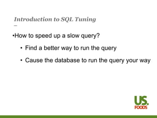
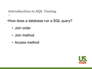
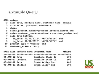
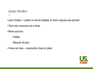
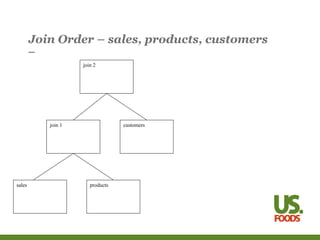
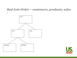
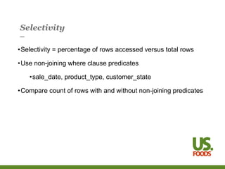
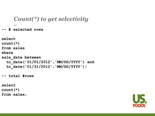
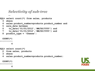
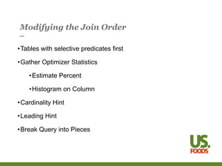
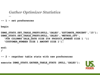
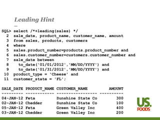
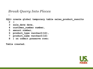
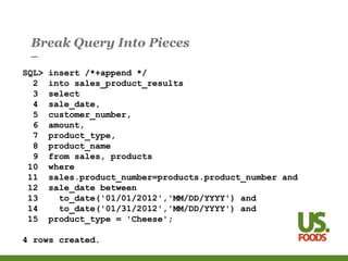
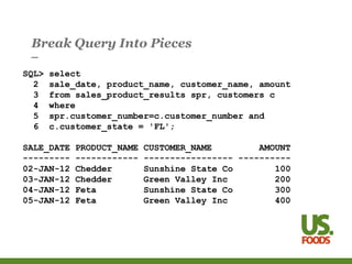
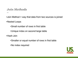
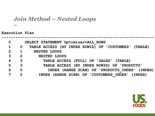
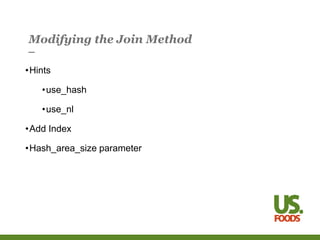
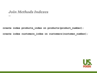
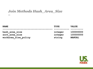
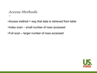
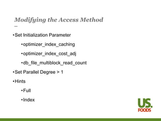
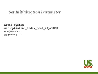
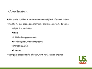
Introduction to SQL Tuning
Brown Bag
Three essential concepts
Introduction to SQL Tuning
•How to speed up a slow query?
• Find a better way to run the query
• Cause the database to run the query your way
Introduction to SQL Tuning
•How does a database run a SQL query?
• Join order
• Join method
• Access method
Example Query
SQL> select
2 sale_date, product_name, customer_name, amount
3 from sales, products, customers
4 where
5 sales.product_number=products.product_number and
6 sales.customer_number=customers.customer_number and
7 sale_date between
8 to_date('01/01/2012','MM/DD/YYYY') and
9 to_date('01/31/2012','MM/DD/YYYY') and
10 product_type = 'Cheese' and
11 customer_state = 'FL';
SALE_DATE PRODUCT_NAME CUSTOMER_NAME AMOUNT
--------- ------------ ----------------- ----------
04-JAN-12 Feta Sunshine State Co 300
02-JAN-12 Chedder Sunshine State Co 100
05-JAN-12 Feta Green Valley Inc 400
03-JAN-12 Chedder Green Valley Inc 200
Join Order
•Join Order = order in which tables in from clause are joined
•Two row sources at a time
•Row source:
•Table
•Result of join
•View as tree – execution tree or plan
Join Order – sales, products, customers
products
sales
join 1 customers
join 2
Join Order as Plan
Execution Plan
----------------------------------------------------------
0 SELECT STATEMENT
1 0 HASH JOIN
2 1 HASH JOIN
3 2 TABLE ACCESS (FULL) OF 'SALES' (TABLE)
4 2 TABLE ACCESS (FULL) OF 'PRODUCTS' (TABLE
5 1 TABLE ACCESS (FULL) OF 'CUSTOMERS' (TABLE)
Bad Join Order – customers, products, sales
products
customers
join 1 sales
join 2
Cartesian Join – all products to all customers
SQL> -- joining products and customers
SQL> -- cartesian join
SQL>
SQL> select
2 product_name,customer_name
3 from products, customers
4 where
5 product_type = 'Cheese' and
6 customer_state = 'FL';
PRODUCT_NAME CUSTOMER_NAME
------------ -----------------
Chedder Sunshine State Co
Chedder Green Valley Inc
Feta Sunshine State Co
Feta Green Valley Inc
Plan with Cartesian Join
Execution Plan
----------------------------------------------------------
0 SELECT STATEMENT Optimizer=ALL_ROWS
1 0 MERGE JOIN (CARTESIAN)
2 1 TABLE ACCESS (FULL) OF 'PRODUCTS' (TABLE)
3 1 BUFFER (SORT)
4 3 TABLE ACCESS (FULL) OF 'CUSTOMERS' (TABLE)
Selectivity
•Selectivity = percentage of rows accessed versus total rows
•Use non-joining where clause predicates
•sale_date, product_type, customer_state
•Compare count of rows with and without non-joining predicates
Count(*) to get selectivity
-- # selected rows
select
count(*)
from sales
where
sale_date between
to_date('01/01/2012','MM/DD/YYYY') and
to_date('01/31/2012','MM/DD/YYYY');
-- total #rows
select
count(*)
from sales;
Selectivity of sub-tree
SQL> select count(*) from sales, products
3 where
4 sales.product_number=products.product_number and
5 sale_date between
6 to_date('01/01/2012','MM/DD/YYYY') and
7 to_date('01/31/2012','MM/DD/YYYY') and
8 product_type = 'Cheese';
COUNT(*)
----------
4
SQL> select count(*)
2 from sales, products
3 where
4 sales.product_number=products.product_number;
COUNT(*)
----------
4
Modifying the Join Order
•Tables with selective predicates first
•Gather Optimizer Statistics
•Estimate Percent
•Histogram on Column
•Cardinality Hint
•Leading Hint
•Break Query into Pieces
Gather Optimizer Statistics
-- 1 - set preferences
begin
DBMS_STATS.SET_TABLE_PREFS(NULL,'SALES','ESTIMATE_PERCENT','10');
DBMS_STATS.SET_TABLE_PREFS(NULL,'SALES','METHOD_OPT',
'FOR COLUMNS SALE_DATE SIZE 254 PRODUCT_NUMBER SIZE 1 '||
'CUSTOMER_NUMBER SIZE 1 AMOUNT SIZE 1');
end;
/
-- 2 - regather table stats with new preferences
execute DBMS_STATS.GATHER_TABLE_STATS (NULL,'SALES');
Cardinality Hint
SQL> select /*+cardinality(sales 1) */
2 sale_date, product_name, customer_name, amount
3 from sales, products, customers
4 where
5 sales.product_number=products.product_number and
6 sales.customer_number=customers.customer_number and
7 sale_date between
8 to_date('01/01/2012','MM/DD/YYYY') and
9 to_date('01/31/2012','MM/DD/YYYY') and
10 product_type = 'Cheese' and
11 customer_state = 'FL';
SALE_DATE PRODUCT_NAME CUSTOMER_NAME AMOUNT
--------- ------------ ----------------- ----------
04-JAN-12 Feta Sunshine State Co 300
02-JAN-12 Chedder Sunshine State Co 100
05-JAN-12 Feta Green Valley Inc 400
03-JAN-12 Chedder Green Valley Inc 200
Plan with Cardinality hint
Execution Plan
----------------------------------------------------------
0 SELECT STATEMENT Optimizer=ALL_ROWS
1 0 HASH JOIN
2 1 HASH JOIN
3 2 TABLE ACCESS (FULL) OF 'SALES' (TABLE)
4 2 TABLE ACCESS (FULL) OF 'PRODUCTS' (TABLE
5 1 TABLE ACCESS (FULL) OF 'CUSTOMERS' (TABLE)
Leading Hint
SQL> select /*+leading(sales) */
2 sale_date, product_name, customer_name, amount
3 from sales, products, customers
4 where
5 sales.product_number=products.product_number and
6 sales.customer_number=customers.customer_number and
7 sale_date between
8 to_date('01/01/2012','MM/DD/YYYY') and
9 to_date('01/31/2012','MM/DD/YYYY') and
10 product_type = 'Cheese' and
11 customer_state = 'FL';
SALE_DATE PRODUCT_NAME CUSTOMER_NAME AMOUNT
--------- ------------ ----------------- ----------
04-JAN-12 Feta Sunshine State Co 300
02-JAN-12 Chedder Sunshine State Co 100
05-JAN-12 Feta Green Valley Inc 400
03-JAN-12 Chedder Green Valley Inc 200
Break Query Into Pieces
SQL> create global temporary table sales_product_results
2 (
3 sale_date date,
4 customer_number number,
5 amount number,
6 product_type varchar2(12),
7 product_name varchar2(12)
8 ) on commit preserve rows;
Table created.
Break Query Into Pieces
SQL> insert /*+append */
2 into sales_product_results
3 select
4 sale_date,
5 customer_number,
6 amount,
7 product_type,
8 product_name
9 from sales, products
10 where
11 sales.product_number=products.product_number and
12 sale_date between
13 to_date('01/01/2012','MM/DD/YYYY') and
14 to_date('01/31/2012','MM/DD/YYYY') and
15 product_type = 'Cheese';
4 rows created.
Break Query Into Pieces
SQL> select
2 sale_date, product_name, customer_name, amount
3 from sales_product_results spr, customers c
4 where
5 spr.customer_number=c.customer_number and
6 c.customer_state = 'FL';
SALE_DATE PRODUCT_NAME CUSTOMER_NAME AMOUNT
--------- ------------ ----------------- ----------
02-JAN-12 Chedder Sunshine State Co 100
03-JAN-12 Chedder Green Valley Inc 200
04-JAN-12 Feta Sunshine State Co 300
05-JAN-12 Feta Green Valley Inc 400
Join Methods
•Join Method = way that data from two sources is joined
•Nested Loops
•Small number of rows in first table
•Unique index on second large table
•Hash Join
•Smaller or equal number of rows in first table
•No index required
Join Method – Nested Loops
Execution Plan
------------------------------------------------------------------
0 SELECT STATEMENT Optimizer=ALL_ROWS
1 0 TABLE ACCESS (BY INDEX ROWID) OF 'CUSTOMERS' (TABLE)
2 1 NESTED LOOPS
3 2 NESTED LOOPS
4 3 TABLE ACCESS (FULL) OF 'SALES' (TABLE)
5 3 TABLE ACCESS (BY INDEX ROWID) OF 'PRODUCTS'
6 5 INDEX (RANGE SCAN) OF 'PRODUCTS_INDEX' (INDEX)
7 2 INDEX (RANGE SCAN) OF 'CUSTOMERS_INDEX' (INDEX)
Join Method – Hash Join
Execution Plan
----------------------------------------------------------
0 SELECT STATEMENT Optimizer=ALL_ROWS
1 0 HASH JOIN
2 1 HASH JOIN
3 2 TABLE ACCESS (FULL) OF 'SALES' (TABLE)
4 2 TABLE ACCESS (FULL) OF 'PRODUCTS'
5 1 TABLE ACCESS (FULL) OF 'CUSTOMERS' (TABLE)
Modifying the Join Method
•Hints
•use_hash
•use_nl
•Add Index
•Hash_area_size parameter
Join Methods Hints
/*+ use_hash(products) use_nl(customers) */
Join Methods Indexes
create index products_index on products(product_number);
create index customers_index on customers(customer_number);
Join Methods Hash_Area_Size
NAME TYPE VALUE
------------------------------------ ----------- ---------
hash_area_size integer 100000000
sort_area_size integer 100000000
workarea_size_policy string MANUAL
Access Methods
•Access method = way that data is retrieved from table
•Index scan – small number of rows accessed
•Full scan – larger number of rows accessed
Modifying the Access Method
•Set Initialization Parameter
•optimizer_index_caching
•optimizer_index_cost_adj
•db_file_multiblock_read_count
•Set Parallel Degree > 1
•Hints
•Full
•Index
Set Initialization Parameter
alter system
set optimizer_index_cost_adj=1000
scope=both
sid='*';
Set Parallel Degree
alter table sales parallel 8;
Full Scan and Index Hints
/*+ full(sales) index(customers) index(products) */
Conclusion
• Use count queries to determine selective parts of where clause
• Modify the join order, join methods, and access methods using
• Optimizer statistics
• Hints
• Initialization parameters
• Breaking the query into pieces
• Parallel degree
• Indexes
• Compare elapsed time of query with new plan to original
Check For Improved Elapsed Time
SQL> set timing on
SQL>
SQL> select …
… removed for clarity …
SALE_DATE PRODUCT_NAME CUSTOMER_NAME AMOUNT
--------- ------------ ----------------- ----------
02-JAN-12 Chedder Sunshine State Co 100
03-JAN-12 Chedder Green Valley Inc 200
04-JAN-12 Feta Sunshine State Co 300
05-JAN-12 Feta Green Valley Inc 400
Elapsed: 00:00:00.00
Further Reading
•Oracle Database Concepts
•Chapter 7 SQL
•Oracle Database Performance Tuning Guide
•Chapter 11 The Query Optimizer
•Chapter 19 Using Optimizer Hints
•Oracle Database Reference
•Chapter 1 Initialization Parameters
•Oracle Database PL/SQL Packages and Types Reference
•Chapter 141 DBMS_STATS
•Cost-Based Oracle Fundamentals - Jonathan Lewis
•http://www.bobbydurrettdba.com/resources/

OracleSQLTuning.ppt

  • 1.
    Introduction to SQLTuning Brown Bag Three essential concepts
  • 2.
    Introduction to SQLTuning •How to speed up a slow query? • Find a better way to run the query • Cause the database to run the query your way
  • 3.
    Introduction to SQLTuning •How does a database run a SQL query? • Join order • Join method • Access method
  • 4.
    Example Query SQL> select 2sale_date, product_name, customer_name, amount 3 from sales, products, customers 4 where 5 sales.product_number=products.product_number and 6 sales.customer_number=customers.customer_number and 7 sale_date between 8 to_date('01/01/2012','MM/DD/YYYY') and 9 to_date('01/31/2012','MM/DD/YYYY') and 10 product_type = 'Cheese' and 11 customer_state = 'FL'; SALE_DATE PRODUCT_NAME CUSTOMER_NAME AMOUNT --------- ------------ ----------------- ---------- 04-JAN-12 Feta Sunshine State Co 300 02-JAN-12 Chedder Sunshine State Co 100 05-JAN-12 Feta Green Valley Inc 400 03-JAN-12 Chedder Green Valley Inc 200
  • 5.
    Join Order •Join Order= order in which tables in from clause are joined •Two row sources at a time •Row source: •Table •Result of join •View as tree – execution tree or plan
  • 6.
    Join Order –sales, products, customers products sales join 1 customers join 2
  • 7.
    Join Order asPlan Execution Plan ---------------------------------------------------------- 0 SELECT STATEMENT 1 0 HASH JOIN 2 1 HASH JOIN 3 2 TABLE ACCESS (FULL) OF 'SALES' (TABLE) 4 2 TABLE ACCESS (FULL) OF 'PRODUCTS' (TABLE 5 1 TABLE ACCESS (FULL) OF 'CUSTOMERS' (TABLE)
  • 8.
    Bad Join Order– customers, products, sales products customers join 1 sales join 2
  • 9.
    Cartesian Join –all products to all customers SQL> -- joining products and customers SQL> -- cartesian join SQL> SQL> select 2 product_name,customer_name 3 from products, customers 4 where 5 product_type = 'Cheese' and 6 customer_state = 'FL'; PRODUCT_NAME CUSTOMER_NAME ------------ ----------------- Chedder Sunshine State Co Chedder Green Valley Inc Feta Sunshine State Co Feta Green Valley Inc
  • 10.
    Plan with CartesianJoin Execution Plan ---------------------------------------------------------- 0 SELECT STATEMENT Optimizer=ALL_ROWS 1 0 MERGE JOIN (CARTESIAN) 2 1 TABLE ACCESS (FULL) OF 'PRODUCTS' (TABLE) 3 1 BUFFER (SORT) 4 3 TABLE ACCESS (FULL) OF 'CUSTOMERS' (TABLE)
  • 11.
    Selectivity •Selectivity = percentageof rows accessed versus total rows •Use non-joining where clause predicates •sale_date, product_type, customer_state •Compare count of rows with and without non-joining predicates
  • 12.
    Count(*) to getselectivity -- # selected rows select count(*) from sales where sale_date between to_date('01/01/2012','MM/DD/YYYY') and to_date('01/31/2012','MM/DD/YYYY'); -- total #rows select count(*) from sales;
  • 13.
    Selectivity of sub-tree SQL>select count(*) from sales, products 3 where 4 sales.product_number=products.product_number and 5 sale_date between 6 to_date('01/01/2012','MM/DD/YYYY') and 7 to_date('01/31/2012','MM/DD/YYYY') and 8 product_type = 'Cheese'; COUNT(*) ---------- 4 SQL> select count(*) 2 from sales, products 3 where 4 sales.product_number=products.product_number; COUNT(*) ---------- 4
  • 14.
    Modifying the JoinOrder •Tables with selective predicates first •Gather Optimizer Statistics •Estimate Percent •Histogram on Column •Cardinality Hint •Leading Hint •Break Query into Pieces
  • 15.
    Gather Optimizer Statistics --1 - set preferences begin DBMS_STATS.SET_TABLE_PREFS(NULL,'SALES','ESTIMATE_PERCENT','10'); DBMS_STATS.SET_TABLE_PREFS(NULL,'SALES','METHOD_OPT', 'FOR COLUMNS SALE_DATE SIZE 254 PRODUCT_NUMBER SIZE 1 '|| 'CUSTOMER_NUMBER SIZE 1 AMOUNT SIZE 1'); end; / -- 2 - regather table stats with new preferences execute DBMS_STATS.GATHER_TABLE_STATS (NULL,'SALES');
  • 16.
    Cardinality Hint SQL> select/*+cardinality(sales 1) */ 2 sale_date, product_name, customer_name, amount 3 from sales, products, customers 4 where 5 sales.product_number=products.product_number and 6 sales.customer_number=customers.customer_number and 7 sale_date between 8 to_date('01/01/2012','MM/DD/YYYY') and 9 to_date('01/31/2012','MM/DD/YYYY') and 10 product_type = 'Cheese' and 11 customer_state = 'FL'; SALE_DATE PRODUCT_NAME CUSTOMER_NAME AMOUNT --------- ------------ ----------------- ---------- 04-JAN-12 Feta Sunshine State Co 300 02-JAN-12 Chedder Sunshine State Co 100 05-JAN-12 Feta Green Valley Inc 400 03-JAN-12 Chedder Green Valley Inc 200
  • 17.
    Plan with Cardinalityhint Execution Plan ---------------------------------------------------------- 0 SELECT STATEMENT Optimizer=ALL_ROWS 1 0 HASH JOIN 2 1 HASH JOIN 3 2 TABLE ACCESS (FULL) OF 'SALES' (TABLE) 4 2 TABLE ACCESS (FULL) OF 'PRODUCTS' (TABLE 5 1 TABLE ACCESS (FULL) OF 'CUSTOMERS' (TABLE)
  • 18.
    Leading Hint SQL> select/*+leading(sales) */ 2 sale_date, product_name, customer_name, amount 3 from sales, products, customers 4 where 5 sales.product_number=products.product_number and 6 sales.customer_number=customers.customer_number and 7 sale_date between 8 to_date('01/01/2012','MM/DD/YYYY') and 9 to_date('01/31/2012','MM/DD/YYYY') and 10 product_type = 'Cheese' and 11 customer_state = 'FL'; SALE_DATE PRODUCT_NAME CUSTOMER_NAME AMOUNT --------- ------------ ----------------- ---------- 04-JAN-12 Feta Sunshine State Co 300 02-JAN-12 Chedder Sunshine State Co 100 05-JAN-12 Feta Green Valley Inc 400 03-JAN-12 Chedder Green Valley Inc 200
  • 19.
    Break Query IntoPieces SQL> create global temporary table sales_product_results 2 ( 3 sale_date date, 4 customer_number number, 5 amount number, 6 product_type varchar2(12), 7 product_name varchar2(12) 8 ) on commit preserve rows; Table created.
  • 20.
    Break Query IntoPieces SQL> insert /*+append */ 2 into sales_product_results 3 select 4 sale_date, 5 customer_number, 6 amount, 7 product_type, 8 product_name 9 from sales, products 10 where 11 sales.product_number=products.product_number and 12 sale_date between 13 to_date('01/01/2012','MM/DD/YYYY') and 14 to_date('01/31/2012','MM/DD/YYYY') and 15 product_type = 'Cheese'; 4 rows created.
  • 21.
    Break Query IntoPieces SQL> select 2 sale_date, product_name, customer_name, amount 3 from sales_product_results spr, customers c 4 where 5 spr.customer_number=c.customer_number and 6 c.customer_state = 'FL'; SALE_DATE PRODUCT_NAME CUSTOMER_NAME AMOUNT --------- ------------ ----------------- ---------- 02-JAN-12 Chedder Sunshine State Co 100 03-JAN-12 Chedder Green Valley Inc 200 04-JAN-12 Feta Sunshine State Co 300 05-JAN-12 Feta Green Valley Inc 400
  • 22.
    Join Methods •Join Method= way that data from two sources is joined •Nested Loops •Small number of rows in first table •Unique index on second large table •Hash Join •Smaller or equal number of rows in first table •No index required
  • 23.
    Join Method –Nested Loops Execution Plan ------------------------------------------------------------------ 0 SELECT STATEMENT Optimizer=ALL_ROWS 1 0 TABLE ACCESS (BY INDEX ROWID) OF 'CUSTOMERS' (TABLE) 2 1 NESTED LOOPS 3 2 NESTED LOOPS 4 3 TABLE ACCESS (FULL) OF 'SALES' (TABLE) 5 3 TABLE ACCESS (BY INDEX ROWID) OF 'PRODUCTS' 6 5 INDEX (RANGE SCAN) OF 'PRODUCTS_INDEX' (INDEX) 7 2 INDEX (RANGE SCAN) OF 'CUSTOMERS_INDEX' (INDEX)
  • 24.
    Join Method –Hash Join Execution Plan ---------------------------------------------------------- 0 SELECT STATEMENT Optimizer=ALL_ROWS 1 0 HASH JOIN 2 1 HASH JOIN 3 2 TABLE ACCESS (FULL) OF 'SALES' (TABLE) 4 2 TABLE ACCESS (FULL) OF 'PRODUCTS' 5 1 TABLE ACCESS (FULL) OF 'CUSTOMERS' (TABLE)
  • 25.
    Modifying the JoinMethod •Hints •use_hash •use_nl •Add Index •Hash_area_size parameter
  • 26.
    Join Methods Hints /*+use_hash(products) use_nl(customers) */
  • 27.
    Join Methods Indexes createindex products_index on products(product_number); create index customers_index on customers(customer_number);
  • 28.
    Join Methods Hash_Area_Size NAMETYPE VALUE ------------------------------------ ----------- --------- hash_area_size integer 100000000 sort_area_size integer 100000000 workarea_size_policy string MANUAL
  • 29.
    Access Methods •Access method= way that data is retrieved from table •Index scan – small number of rows accessed •Full scan – larger number of rows accessed
  • 30.
    Modifying the AccessMethod •Set Initialization Parameter •optimizer_index_caching •optimizer_index_cost_adj •db_file_multiblock_read_count •Set Parallel Degree > 1 •Hints •Full •Index
  • 31.
    Set Initialization Parameter altersystem set optimizer_index_cost_adj=1000 scope=both sid='*';
  • 32.
    Set Parallel Degree altertable sales parallel 8;
  • 33.
    Full Scan andIndex Hints /*+ full(sales) index(customers) index(products) */
  • 34.
    Conclusion • Use countqueries to determine selective parts of where clause • Modify the join order, join methods, and access methods using • Optimizer statistics • Hints • Initialization parameters • Breaking the query into pieces • Parallel degree • Indexes • Compare elapsed time of query with new plan to original
  • 35.
    Check For ImprovedElapsed Time SQL> set timing on SQL> SQL> select … … removed for clarity … SALE_DATE PRODUCT_NAME CUSTOMER_NAME AMOUNT --------- ------------ ----------------- ---------- 02-JAN-12 Chedder Sunshine State Co 100 03-JAN-12 Chedder Green Valley Inc 200 04-JAN-12 Feta Sunshine State Co 300 05-JAN-12 Feta Green Valley Inc 400 Elapsed: 00:00:00.00
  • 36.
    Further Reading •Oracle DatabaseConcepts •Chapter 7 SQL •Oracle Database Performance Tuning Guide •Chapter 11 The Query Optimizer •Chapter 19 Using Optimizer Hints •Oracle Database Reference •Chapter 1 Initialization Parameters •Oracle Database PL/SQL Packages and Types Reference •Chapter 141 DBMS_STATS •Cost-Based Oracle Fundamentals - Jonathan Lewis •http://www.bobbydurrettdba.com/resources/

Editor's Notes

  • #2 The key word here is “Introduction”. SQL tuning in Oracle is a vast subject which would require multiple week long classes and that might not be enough. This talk is intended to be the first in a series to train US Foods DBAs and Developers in Oracle SQL tuning. I’ve tried to find a place to start talking about SQL tuning and I think I’ve found the three fundamental concepts which are at the heart of all Oracle SQL tuning. The plan is to touch on all three topics and give practical examples of how to tune queries using this knowledge. Even though this is an introductory talk and can’t go into much depth I want to leave people with a few practical tools they can use right after hearing this talk.
  • #3 The key thing about any SQL database is that the user doesn’t specify how the database will run the query. The database figures that out for you. In some cases the database runs your query very slowly. In that case you need to look at how the database is running the query and then find a different way to run it that you think is faster. Then you have to find a way to make the database use your preferred method. Lastly you have to test the query the new way to make sure it really is faster!
  • #4 The three essential concepts behind Oracle SQL tuning – and most likely all SQL tuning – are join order, join method and access method. Rest of talk is broken up into these three sections. I talk about how to figure out best choices for each and then give multiple methods to change the databases choices to be the one you think is best. Ultimately of course you have to test in the end to be sure you were right.
  • #5 This is a fictional sales application. Three tables – sales, products, and customers joined on product_number and customer number. It was key to have an example with three tables so you can show the results of one join being joined to a third table.
  • #6 key is that two things are joined together at a time – two tables, or the results of a join and a table, or the results of two earlier joins. Oracle calls these row sources so a join is always a join of two row sources – table or earlier join
  • #7 sales and products are joined first and then result is joined to customers. Key here is that sales is the first component of the join and products is second. We will talk later about how the order is important. i.e. in a hash join the first table makes the hash table and the second probes it so sales, products, customers join order differs from products, sales, customers
  • #8 tree is rotated to the left 90 degrees and then flipped across its horizontal axis to get the plan. The indentation shows how deep into the tree you are. The sales table is first in the hash join. The inner hash join is first in the second join to the customers table.
  • #9 The point of this example is to show a join order that is obviously bad. A cartesian join of customers and products would take forever if these were large tables. My simple example only has two rows in each table so it is fast, but in the real world with 100,000 customers and 100,000 products the resulting join would have 10 billion resulting rows
  • #10 This query mimics the subtree in the plan with the bad join order. products and customers are joined but there is no predicate in the where clause that relates the two tables. So, it joins every product with every customer. Since there are two of each we get 2 times 2 = 4 total.
  • #11 Notice the word “Cartesian” in the plan. Every products rows joined to every customers.
  • #12 This is really the crux of the talk. Use count(*) queries on pieces of the query to find out how many rows are really returned for the criteria specified in the where clause. So, in our example for sales the January 2012 date range how selective is that? If there are ten years of data in the sales table – 120 months then one month out of 120 is a selectivity of 1/120th. If the sales table only has two months data then one month would be 50% selective. The whole point of this talk is to find some huge improvement in query performance so the key is to find some part of the query’s where clause that is super selective and then adjust the join order, join methods, and access methods to take advantage of that fact. Key here is the assumption of the talk at this point is that you have a query that can be run fast but the optimizer is running it very slow. The only way this would happen is if the optimizer didn’t know that the predicates were so selective. Can’t get into why this in this talk but they key is that the optimizer is built for speed. It can’t take forever to figure out how to run the query so there has to be limits on how well it can choose the plan. Also, you may need to change things – like add indexes – to give the optimizer a good way to run the query anyway. Anyway, the point is to find some super selective part of the query and then take advantage of it – really the main point of the talk. This is the heart of query tuning.
  • #13 This gets the selectivity of the where clause predicates on a single table – sales in this case. You could do the same thing for products and customers. Sales only has a criteria on sale_date so we want to see how many of the sales rows meet that criteria. Do count on sales with the criteria and without it.
  • #14 This is trickier to explain, but the point is that you will have subtrees joined and some subtrees may return just a few rows. You will end up putting this subtree earlier in the join order and it will affect your choice of join method and access method. In our three table example we only have three possible subtrees – sales-products, sales-customers, products-customers. This example is the sales-products one. Note that the comparison is between the join with the sale_date and product_type criteria and without. Imagine that you had just started having cheese products in February 2012. The combination of January 2012 and Cheese would return 0 rows, but each individual condition – jan 2012 or cheese would return rows. So, a combined condition may be unexpectedly very selective and if you find one like this then you have the basis for dramatic performance improvement by exploiting this knowledge in your choice of join order, join method, and access method.
  • #15 Key here is that if you have some very selective predicates you want the table(s) these are on to be at the front of the join order. That way there are fewer rows to be joined to the later tables and it makes the whole query run faster. This is where the really practical details come in. Each of these isn’t the full story. I just give a quick example of each so people can do further research into it. But at least it gives you some tools to use right away to improve query performance. Estimate percents – with greater percents you will have more accurate view of column values. with histogram you see exceptional values. cardinality hint overrides optimizer’s estimate of number of rows from a table that will match the where clause criteria. Leading just makes that table go first. Note that hints are just that – hints – really the optimizer can do whatever it wants. It may ignore hints. Last thing breaking up queries is huge. So simple yet really powerful. You become the optimizer.
  • #16 In 11g you can set preferences on a table. Set estimate percentage on sales to 10% if default is less and not giving accurate cardinality estimates. METHOD_OPT tells which columns to have histograms – size is number of buckets. 1 bucket histogram is essentially the norm – no histogram. 254 buckets is the max. sales_date here has that. Once prefs are set can gather stats without specifying estimate_percent or method_opt and it will use the preference. Also, automatic stats job will use it. The point here is that if the optimizer knows how selective the predicates are it will set the associated table to the front of the join order. you can adjust the optimizer stats to give the optimizer better information and that results in a better join order.
  • #17 Cardinality is undocumented hint. Tells the optimizer that the sales table will return one row – i.e. january 2012 has one row. Reality here is that there are 4 rows. But, underestimating causes sales to go first in the join order because it makes the optimizer think that sales has fewer rows returned than products or customers. Note that the optimizer still determines the rest of the details of the join order – which is next, customers or products?
  • #18 Sales joins to products. result joins to customers. I don’t show the cardinality here for space but in the real output I copied this from cardinality of sales was listed as 1.
  • #19 Note about hints. In all my examples I have the name of the table to keep it simple. If you have a table alias you have to use the alias name. i.e. leading(s) if you have from sales s. This has the same effect as the cardinality hint except here you tell the optimizer that sales should be the first table in the join order. Isn’t a guarantee but the optimizer takes the hint into account. Plan is the same as for the cardinality hint.
  • #20 Powerful technique. Two big datawarehouse batch scripts resolved this way. Take the full query and break it into its smallest pieces – joining at most two tables at a time together and saving the results in a global temporary table. you become the optimizer. you can also use hints and other techniques on the smaller queries. This slide show creation of the table to save the results of the join between sales and products.
  • #21 This is the join between sales and products. It has the join condition on product_number to relate the tables and the conditions on sale_date and product_type from the original query. The columns are all the columns needed for the final result and the join to customers. In real script you need a commit after this insert but I left it out for clarity.
  • #22 Final query – same result. Here you join customers to the temp table on customer_number and include the customer_state criteria. The select column names are the same. what we have done here is force the join order to be sales-products-customers. Note that we have not forced the order of the tables in each join but have left that up to the optimizer. a leading hint could force that as well.
  • #23 Two methods I mainly use when forcing a join method – nested loops or hash join. not talking about merge join for simplicity and because I really don’t use it. nested loops – for each row in the first table probe the second table based on join columns hash join – load rows from first table into a hash table, probe it with every row from second table Key here is selectivity and cardinality. index on join columns is good for nested loops. unique index is just ideal, not required. Gives biggest improvement. Again, looking for big bang hash join even large numbers of rows can be in hash table. mostly on disk but buffered in pga memory.
  • #24 full scan of sales, probing products using products_index. result probes customers using customers_index. can mix and match. this is all nested loops for demonstration Note that the predicates are applied as well. Only the jan 2012 sales rows probe products. Only the cheese products prob customers. Only the florida customers are returned.
  • #25 Same plan we have seen before. all hash joins. all of sales read into hash table (all the january 2012 sales that is). cheese products probe hash table. result of this join loaded into a new hash table. florida customers probe hash table.
  • #26 if you have looked at the selectivity of the predicates and know how many rows each table will return you can change the join order. hints explicitly tell the optimizer which type to use. adding an index to the table with larger number of rows will encourage nested loops if the columns indexed are the join columns. Manually setting the pga memory hash area to a larger number encourages hash joins over nested loops
  • #27 inner (right) table of join
  • #28 shows how to create indexes on the columns used to join sales to products and customers. These enable a nested loops join to these tables to be efficient where they are joined on the indexed column. I don’t specify unique indexes here for simplicity but if the columns uniquely identify the rows it is the same effect regardless. You might want a combination of use_nl hint and index to force nl join. also you might want a combo of a full hint and use_hash hint to force a good hash join.
  • #29 These are settings in a real production system. Wanted to encourage hash joins and speed them up with the use of more PGA memory. Only challenge here is that wth a 100 meg hash and sort area that is per session. So with many sessions you could eat up a lot of memory. That is the downside with manually setting these memory parameters.
  • #30 There are a lot of different access methods not talked about here – partitioning, compression, bitmap indexes, clusters, etc. But, the difference between and plan b-tree index range scan and a full table scan is a fundamental concept which really applies to all the others anyway. The bottom line is how many rows or what percentage of the rows from the table are being pulled in. Small number of rows = index, large in full scan. Goes back to initial count(*) queries. have to know number of rows really returned after applying the where clause predicates. Note how these relate back to join order and join method. You want the index scan on the second table of a nested loops join. In many cases a full scan is ok for both tables of a hash join. you can still use an index scan for the hash joined tables and for the first table in a nested loops if the where clause predicates are on indexed columns.
  • #31 init parameters make indexes versus full scans overall more or less likely. parallel degree > 1 makes full scans more likely. hints encourage one or the other.
  • #32 Used this on an exadata system to encourage full scans – which get turned into Exadata smart scans. normal value of optimizer_index_cost_adj is 100. 1000 means indexes cost 10 times as much as normal so that gets factored into the optimizer’s choices so a full scan is more likely. note that it doesn’t eliminate index use. it just discourages it.
  • #33 with noparallel optimizer thinks a full scan takes X seconds. with parallel 8 it thinks it takes X/8. So, this makes it 8 times more likely to do a full scan.
  • #34 hints encourage use of the given access method. here I’m using the format index(table name). can also be index(table_name index_name). also table names would be the aliases. I left it this way for simplicity.
  • #35 This is good summary – do counts first, tweek the join order, join method, access method based on the counts to get the low row count things where they need to be. Double check everything with elapsed time. Get elapsed time with no changes – run multiple times. Then get elapsed time after with multiple runs.
  • #36 sqlplus set timing on to measure elapsed time. This is the real measure of success. After all the analysis and making sure you have the join order, join methods and access methods you BELIEVE are best then have to check the real elapsed time. If you find some extreme selectivity that the original plan didn’t exploit then your new run time could be 1000 time less than it was before. Elapsed time is the proof. all the rest is theory. test everything twice. don’t believe anything you don’t test for yourself.
  • #37 Chapters of the manuals that relate to topic. SQL reference also has hints under comments. Jonathan Lewis’s book was great help to me.