numpy.pdf

6.1 Introduction
NumPy stands for ‘Numerical Python’. It is a
package for data analysis and scientific computing
with Python. NumPy uses a multidimensional
array object, and has functions and tools
for working with these arrays. The powerful
n-dimensional array in NumPy speeds-up data
processing. NumPy can be easily interfaced with
other Python packages and provides tools for
integrating with other programming languages
like C, C++ etc.
Introduction
to NumPy
Chapter
6
“The goal is to turn data into information,
and information into insight.”
— Carly Fiorina
In this chapter
»
» Introduction
»
» Array
»
» NumPy Array
»
» Indexing and Slicing
»
» Operations on Arrays
»
» Concatenating Arrays
»
» Reshaping Arrays
»
» Splitting Arrays
»
» Statistical Operations
on Arrays
»
» Loading Arrays from
Files
»
» Saving NumPy Arrays
in Files on Disk
Chap 6.indd 95 19-Jul-19 3:43:32 PM
2022-23

96 Informatics Practices – Class XI
Installing NumPy
NumPy can be installed by typing following command:
pip install NumPy
6.2 Array
We have learnt about various data types like list, tuple,
and dictionary. In this chapter we will discuss another
datatype ‘Array’. An array is a data type used to store
multiple values using a single identifier (variable name).
An array contains an ordered collection of data elements
where each element is of the same type and can be
referenced by its index (position).
The important characteristics of an array are:
• Each element of the array is of same data
type, though the values stored in them may be
different.
• The entire array is stored contiguously in
memory. This makes operations on array fast.
• Each element of the array is identified or
referred using the name of the Array along with
the index of that element, which is unique for
each element. The index of an element is an
integral value associated with the element,
based on the element’s position in the array.
For example consider an array with 5 numbers:
[ 10, 9, 99, 71, 90 ]
Here, the 1st value in the array is 10 and has the
index value [0] associated with it; the 2nd
value in the
array is 9 and has the index value [1] associated with
it, and so on. The last value (in this case the 5th
value)
in this array has an index [4]. This is called zero based
indexing. This is very similar to the indexing of lists in
Python. The idea of arrays is so important that almost
all programming languages support it in one form or
another.
6.3 NumPy Array
NumPy arrays are used to store lists of numerical data,
vectors and matrices. The NumPy library has a large set of
routines (built-in functions) for creating, manipulating,
and transforming NumPy arrays. Python language also
has an array data structure, but it is not as versatile,
efficient and useful as the NumPy array. The NumPy
Contiguous memory
allocation:
The memory space
must be divided
into the fined sized
position and each
position is allocated
to a single data only.
Now Contiguous
Memory Allocation:
Divide the data into
several blocks and
place in different
parts of the memory
according to the
availability of memory
space.
Chap 6.indd 96 19-Jul-19 3:43:32 PM
2022-23

Introduction to NumPy 97
array is officially called ndarray but commonly known
as array. In rest of the chapter, we will be referring to
NumPy array whenever we use “array”. following are few
differences between list and Array.
6.3.1 Difference Between List and Array
List Array
List can have elements of different data
types for example, [1,3.4, ‘hello’, ‘a@’]
All elements of an array are of same data type for
example, an array of floats may be: [1.2, 5.4, 2.7]
Elements of a list are not stored
contiguously in memory.
Array elements are stored in contiguous memory
locations. This makes operations on arrays faster than
lists.
Listsdonotsupportelementwiseoperations,
for example, addition, multiplication, etc.
because elements may not be of same type.
Arrays support element wise operations. For example,
if A1 is an array, it is possible to say A1/3 to divide
each element of the array by 3.
Lists can contain objects of different
datatype that Python must store the type
information for every element along with its
element value. Thus lists take more space
in memory and are less efficient.
NumPy array takes up less space in memory as
compared to a list because arrays do not require to
store datatype of each element separately.
List is a part of core Python. Array (ndarray) is a part of NumPy library.
6.3.2 Creation of NumPy Arrays from List
There are several ways to create arrays. To create an
array and to use its methods, first we need to import the
NumPy library.
#NumPy is loaded as np (we can assign any
#name), numpy must be written in lowercase
>>> import numpy as np
The NumPy’s array() function converts a given list
into an array. For example,
#Create an array called array1 from the
#given list.
>>> array1 = np.array([10,20,30])
#Display the contents of the array
>>> array1
array([10, 20, 30])
• Creating a 1-D Array
An array with only single row of elements is called
1-D array. Let us try to create a 1-D array from
a list which contains numbers as well as strings.
>>> array2 = np.array([5,-7.4,'a',7.2])
>>> array2
Chap 6.indd 97 19-Jul-19 3:43:32 PM
2022-23

array(['5', '-7.4', 'a', '7.2'],
dtype='<U32')
Observe that since there is a string value in the
list, all integer and float values have been promoted to
string, while converting the list to array.
Note: U32 means Unicode-32 data type.
• Creating a 2-D Array
We can create a two dimensional (2-D) arrays by
passing nested lists to the array() function.
Example 6.1
>>> array3 = np.array([[2.4,3],
[4.91,7],[0,-1]])
>>> array3
array([[ 2.4 , 3. ],
[ 4.91, 7. ],
[ 0. , -1. ]])
Observe that the integers 3, 7, 0 and -1 have been
promoted to floats.
6.3.3 Attributes of NumPy Array
Some important attributes of a NumPy ndarray object are:
i) ndarray.ndim: gives the number of dimensions
of the array as an integer value. Arrays can be
1-D, 2-D or n-D. In this chapter, we shall focus
on 1-D and 2-D arrays only. NumPy calls the
dimensions as axes (plural of axis). Thus, a 2-D
array has two axes. The row-axis is called axis-0
and the column-axis is called axis-1. The number
of axes is also called the array’s rank.
Example 6.2
>>> array1.ndim
1
>>> array3.ndim
2
ii) ndarray.shape: It gives the sequence of integers
indicating the size of the array for each dimension.
Example 6.3
# array1 is 1D-array, there is nothing
# after , in sequence
>>> array1.shape
(3,)
>>> array2.shape
(4,)
>>> array3.shape
(3, 2)
A common mistake
occurs while passing
argument to array() if
we forget to put square
brackets. Make sure
only a single argument
containing list of
values is passed.
#incorrect way
>>> a =
np.array(1,2,3,4)
#correct way
>>> a =
np.array([1,2,3,4])
A list is called nested
list when each
element is a list itself.
Chap 6.indd 98 19-Jul-19 3:43:32 PM
2022-23

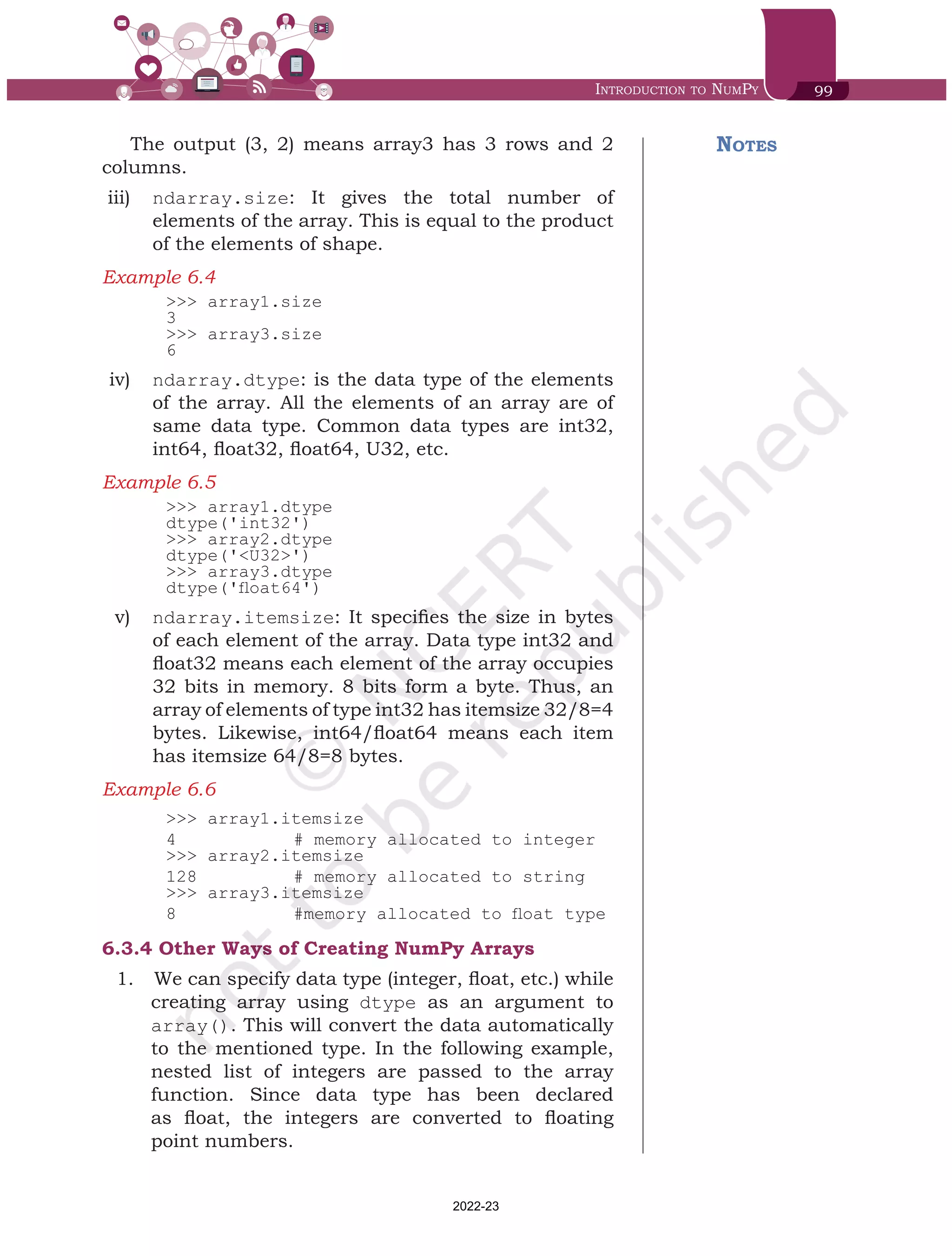
The output (3, 2) means array3 has 3 rows and 2
columns.
iii) ndarray.size: It gives the total number of
elements of the array. This is equal to the product
of the elements of shape.
Example 6.4
>>> array1.size
3
>>> array3.size
6
iv) ndarray.dtype: is the data type of the elements
of the array. All the elements of an array are of
same data type. Common data types are int32,
int64, float32, float64, U32, etc.
Example 6.5
>>> array1.dtype
dtype('int32')
>>> array2.dtype
dtype('<U32>')
>>> array3.dtype
dtype('float64')
v) ndarray.itemsize: It specifies the size in bytes
of each element of the array. Data type int32 and
float32 means each element of the array occupies
32 bits in memory. 8 bits form a byte. Thus, an
array of elements of type int32 has itemsize 32/8=4
bytes. Likewise, int64/float64 means each item
has itemsize 64/8=8 bytes.
Example 6.6
>>> array1.itemsize
4 # memory allocated to integer
>>> array2.itemsize
128 # memory allocated to string
>>> array3.itemsize
8 #memory allocated to float type
6.3.4 Other Ways of Creating NumPy Arrays
1. We can specify data type (integer, float, etc.) while
creating array using dtype as an argument to
array(). This will convert the data automatically
to the mentioned type. In the following example,
nested list of integers are passed to the array
function. Since data type has been declared
as float, the integers are converted to floating
point numbers.
Notes
Chap 6.indd 99 19-Jul-19 3:43:32 PM
2022-23

>>> array4 = np.array( [ [1,2], [3,4] ],
dtype=float)
>>> array4
array([[1., 2.],
[3., 4.]])
2. We can create an array with all elements initialised
to 0 using the function zeros(). By default, the
data type of the array created by zeros() is float.
The following code will create an array with 3 rows
and 4 columns with each element set to 0.
>>> array5 = np.zeros((3,4))
>>> array5
array([[0., 0., 0., 0.],
[0., 0., 0., 0.],
[0., 0., 0., 0.]])
3. We can create an array with all elements initialised
to 1 using the function ones(). By default, the
data type of the array created by ones() is float.
The following code will create an array with 3 rows
and 2 columns.
>>> array6 = np.ones((3,2))
>>> array6
array([[1., 1.],
[1., 1.],
[1., 1.]])
4. We can create an array with numbers in a given
range and sequence using the arange() function.
This function is analogous to the range() function
of Python.
>>> array7 = np.arange(6)
# an array of 6 elements is created with
start value 5 and step size 1
>>> array7
array([0, 1, 2, 3, 4, 5])
# Creating an array with start value -2, end
# value 24 and step size 4
>>> array8 = np.arange( -2, 24, 4 )
>>> array8
array([-2, 2, 6, 10, 14, 18, 22])
6.4 Indexing and Slicing
NumPy arrays can be indexed, sliced and iterated over.
6.4.1 Indexing
We have learnt about indexing single-dimensional
array in section 6.2. For 2-D arrays indexing for both
dimensions starts from 0, and each element is referenced
through two indexes i and j, where i represents the row
number and j represents the column number.
Think and Reflect
When we may require
to create an array
initialised to zeros or
ones?
Chap 6.indd 100 19-Jul-19 3:43:32 PM
2022-23

Table 6.1 Marks of students in different subjects
Name Maths English Science
Ramesh 78 67 56
Vedika 76 75 47
Harun 84 59 60
Prasad 67 72 54
Consider Table 6.1 showing marks obtained by
students in three different subjects. Let us create an
array called marks to store marks given in three subjects
for four students given in this table. As there are 4
students (i.e. 4 rows) and 3 subjects (i.e. 3 columns),
the array will be called marks[4][3]. This array can
store 4*3 = 12 elements.
Here, marks[i,j] refers to the element at (i+1)th
row
and (j+1)th
column because the index values start at 0.
Thus marks[3,1] is the element in 4th
row and second
column which is 72 (marks of Prasad in English).
# accesses the element in the 1st
row in
# the 3rd
column
>>> marks[0,2]
56
>>> marks [0,4]
index Out of Bound "Index Error". Index 4
is out of bounds for axis with size 3
6.4.2 Slicing
Sometimes we need to extract part of an array. This is
done through slicing. We can define which part of the
array to be sliced by specifying the start and end index
values using [start : end] along with the array name.
Example 6.7
>>> array8
array([-2, 2, 6, 10, 14, 18, 22])
# excludes the value at the end index
>>> array8[3:5]
array([10, 14])
# reverse the array
>>> array8[ : : -1]
array([22, 18, 14, 10, 6, 2, -2])
Notes
Chap 6.indd 101 19-Jul-19 3:43:32 PM
2022-23

Now let us see how slicing is done for 2-D arrays.
For this, let us create a 2-D array called array9 having
3 rows and 4 columns.
>>> array9 = np.array([[ -7, 0, 10, 20],
[ -5, 1, 40, 200],
[ -1, 1, 4, 30]])
# access all the elements in the 3rd
column
>>> array9[0:3,2]
array([10, 40, 4])
Note that we are specifying rows in the range 0:3
because the end value of the range is excluded.
# access elements of 2nd
and 3rd
row from 1st
# and 2nd
column
>>> array9[1:3,0:2]
array([[-5, 1],
[-1, 1]])
If row indices are not specified, it means all the rows
are to be considered. Likewise, if column indices are
not specified, all the columns are to be considered.
Thus, the statement to access all the elements in the 3rd
column can also be written as:
>>>array9[:,2]
array([10, 40, 4])
6.5 Operations on Arrays
Once arrays are declared, we con access it's element
or perform certain operations the last section, we
learnt about accessing elements. This section describes
multiple operations that can be applied on arrays.
6.5.1 Arithmetic Operations
Arithmetic operations on NumPy arrays are fast and
simple. When we perform a basic arithmetic operation
like addition, subtraction, multiplication, division etc. on
two arrays, the operation is done on each corresponding
pair of elements. For instance, adding two arrays will
result in the first element in the first array to be added
to the first element in the second array, and so on.
Consider the following element-wise operations on two
arrays:
>>> array1 = np.array([[3,6],[4,2]])
>>> array2 = np.array([[10,20],[15,12]])
Notes
Chap 6.indd 102 19-Jul-19 3:43:32 PM
2022-23

#Element-wise addition of two matrices.
>>> array1 + array2
array([[13, 26],
[19, 14]])
#Subtraction
>>> array1 - array2
array([[ -7, -14],
[-11, -10]])
#Multiplication
>>> array1 * array2
array([[ 30, 120],
[ 60, 24]])
#Matrix Multiplication
>>> array1 @ array2
array([[120, 132],
[ 70, 104]])
#Exponentiation
>>> array1 ** 3
array([[ 27, 216],
[ 64, 8]], dtype=int32)
#Division
>>> array2 / array1
array([[3.33333333, 3.33333333],
[3.75 , 6. ]])
#Element wise Remainder of Division
#(Modulo)
>>> array2 % array1
array([[1, 2],
[3, 0]], dtype=int32)
It is important to note that for element-wise
operations, size of both arrays must be same. That is,
array1.shape must be equal to array2.shape.
6.5.2 Transpose
Transposing an array turns its rows into columns and
columns into rows just like matrices in mathematics.
#Transpose
>>> array3 = np.array([[10,-7,0, 20],
[-5,1,200,40],[30,1,-1,4]])
>>> array3
array([[ 10, -7, 0, 20],
[ -5, 1, 200, 40],
[ 30, 1, -1, 4]])
Notes
Chap 6.indd 103 19-Jul-19 3:43:32 PM
2022-23

# the original array does not change
>>> array3.transpose()
array([[ 10, -5, 30],
[ -7, 1, 1],
[ 0, 200, -1],
[ 20, 40, 4]])
6.5.3 Sorting
Sorting is to arrange the elements of an array in
hierarchical order either ascending or descending. By
default, numpy does sorting in ascending order.
>>> array4 = np.array([1,0,2,-3,6,8,4,7])
>>> array4.sort()
>>> array4
array([-3, 0, 1, 2, 4, 6, 7, 8])
In 2-D array, sorting can be done along either of the
axes i.e., row-wise or column-wise. By default, sorting
is done row-wise (i.e., on axis = 1). It means to arrange
elements in each row in ascending order. When axis=0,
sorting is done column-wise, which means each column
is sorted in ascending order.
>>> array4 = np.array([[10,-7,0, 20],
[-5,1,200,40],[30,1,-1,4]])
>>> array4
array([[ 10, -7, 0, 20],
[ -5, 1, 200, 40],
[ 30, 1, -1, 4]])
#default is row-wise sorting
>>> array4.sort()
>>> array4
array([[ -7, 0, 10, 20],
[ -5, 1, 40, 200],
[ -1, 1, 4, 30]])
>>> array5 = np.array([[10,-7,0, 20],
[-5,1,200,40],[30,1,-1,4]])
#axis =0 means column-wise sorting
>>> array5.sort(axis=0)
>>> array5
array([[ -5, -7, -1, 4],
[ 10, 1, 0, 20],
[ 30, 1, 200, 40]])
6.6 Concatenating Arrays
Concatenation means joining two or more arrays.
Concatenating 1-D arrays means appending the
sequences one after another. NumPy.concatenate()
Notes
Chap 6.indd 104 19-Jul-19 3:43:32 PM
2022-23

function can be used to concatenate two or more
2-D arrays either row-wise or column-wise. All the
dimensions of the arrays to be concatenated must match
exactly except for the dimension or axis along which
they need to be joined. Any mismatch in the dimensions
results in an error. By default, the concatenation of the
arrays happens along axis=0.
Example 6.8
>>> array1 = np.array([[10, 20], [-30,40]])
>>> array2 = np.zeros((2, 3), dtype=array1.
dtype)
>>> array1
array([[ 10, 20],
[-30, 40]])
>>> array2
array([[0, 0, 0],
[0, 0, 0]])
>>> array1.shape
(2, 2)
>>> array2.shape
(2, 3)
>>> np.concatenate((array1,array2), axis=1)
array([[ 10, 20, 0, 0, 0],
[-30, 40, 0, 0, 0]])
>>> np.concatenate((array1,array2), axis=0)
Traceback (most recent call last):
File "<pyshell#3>", line 1, in <module>
np.concatenate((array1,array2))
ValueError: all the input array dimensions
except for the concatenation axis must
match exactly
6.7 Reshaping Arrays
We can modify the shape of an array using the reshape()
function. Reshaping an array cannot be used to change
the total number of elements in the array. Attempting
to change the number of elements in the array using
reshape() results in an error.
Example 6.9
>>> array3 = np.arange(10,22)
>>> array3
array([10, 11, 12, 13, 14, 15, 16, 17, 18,
19, 20, 21])
Notes
Chap 6.indd 105 19-Jul-19 3:43:32 PM
2022-23

>>> array3.reshape(3,4)
array([[10, 11, 12, 13],
[14, 15, 16, 17],
[18, 19, 20, 21]])
>>> array3.reshape(2,6)
array([[10, 11, 12, 13, 14, 15],
[16, 17, 18, 19, 20, 21]])
6.8 Splitting Arrays
We can split an array into two or more subarrays.
numpy.split() splits an array along the specified axis.
We can either specify sequence of index values where an
array is to be split; or we can specify an integer N, that
indicates the number of equal parts in which the array
is to be split, as parameter(s) to the NumPy.split()
function. By default, NumPy.split() splits along axis =
0. Consider the array given below:
>>> array4
array([[ 10, -7, 0, 20],
[ -5, 1, 200, 40],
[ 30, 1, -1, 4],
[ 1, 2, 0, 4],
[ 0, 1, 0, 2]])
# [1,3] indicate the row indices on which
# to split the array
>>> first, second, third = numpy split(array4,
[1, 3])
# array4 is split on the first row and
# stored on the sub-array first
>>> first
array([[10, -7, 0, 20]])
# array4 is split after the first row and
# upto the third row and stored on the
# sub-array second
>>> second
array([[ -5, 1, 200, 40],
[ 30, 1, -1, 4]])
# the remaining rows of array4 are stored
# on the sub-array third
>>> third
array([[1, 2, 0, 4],
[0, 1, 0, 2]])
Notes
Chap 6.indd 106 19-Jul-19 3:43:32 PM
2022-23

#[1, 2], axis=1 give the columns indices
#along which to split
>>> firstc, secondc, thirdc =numpy split(array4,
[1, 2], axis=1)
>>> firstc
array([[10],
[-5],
[30],
[ 1],
[ 0]])
>>> secondc
array([[-7],
[ 1],
[ 1],
[ 2],
[ 1]])
>>> thirdc
array([[ 0, 20],
[200, 40],
[ -1, 4],
[ 0, 4],
[ 0, 2]])
# 2nd
parameter 2 implies array is to be
# split in 2 equal parts axis=1 along the
# column axis
>>> firsthalf, secondhalf =np.split(array4,2,
axis=1)
>>> firsthalf
array([[10, -7],
[-5, 1],
[30, 1],
[ 1, 2],
[ 0, 1]])
>>> secondhalf
array([[ 0, 20],
[200, 40],
[ -1, 4],
[ 0, 4],
[ 0, 2]])
6.9 Statistical Operations on Arrays
NumPy provides functions to perform many useful
statistical operations on arrays. In this section, we will
apply the basic statistical techniques called descriptive
statistics that we have learnt in chapter 5.
Notes
Chap 6.indd 107 19-Jul-19 3:43:32 PM
2022-23

Let us consider two arrays:
>>> arrayA = np.array([1,0,2,-3,6,8,4,7])
>>> arrayB = np.array([[3,6],[4,2]])
1. The max() function finds the maximum element
from an array.
# max element form the whole 1-D array
>>> arrayA.max()
8
# max element form the whole 2-D array
>>> arrayB.max()
6
# if axis=1, it gives column wise maximum
>>> arrayB.max(axis=1)
array([6, 4])
# if axis=0, it gives row wise maximum
>>> arrayB.max(axis=0)
array([4, 6])
2. The min() function finds the minimum element
from an array.
>>> arrayA.min()
-3
>>> arrayB.min()
2
>>> arrayB.min(axis=0)
array([3, 2])
3. The sum() function finds the sum of all elements
of an array.
>>> arrayA.sum()
25
>>> arrayB.sum()
15
#axis is used to specify the dimension
#on which sum is to be made. Here axis = 1
#means the sum of elements on the first row
>>> arrayB.sum(axis=1)
array([9, 6])
4. The mean() function finds the average of elements
of the array.
>>> arrayA.mean()
3.125
>>> arrayB.mean()
3.75
>>> arrayB.mean(axis=0)
array([3.5, 4. ])
>>> arrayB.mean(axis=1)
array([4.5, 3. ])
5. The std() function is used to find standard
deviation of an array of elements.
>>> arrayA.std()
3.550968177835448
Notes
Chap 6.indd 108 19-Jul-19 3:43:32 PM
2022-23

>>> arrayB.std()
1.479019945774904
>>> arrayB.std(axis=0)
array([0.5, 2. ])
>>> arrayB.std(axis=1)
array([1.5, 1. ])
6.10 Loading Arrays from Files
Sometimes, we may have data in files and we may need
to load that data in an array for processing. numpy.
loadtxt() and numpy.genfromtxt()are the two
functions that can be used to load data from text files.
The most commonly used file type to handle large amount
of data is called CSV (Comma Separated Values).
Each row in the text file must have the same number
of values in order to load data from a text file into a
numpy array. Let us say we have the following data in a
text file named data.txt stored in the folder C:/NCERT.
RollNo Marks1 Marks2 Marks3
1, 36, 18, 57
2, 22, 23, 45
3, 43, 51, 37
4, 41, 40, 60
5, 13, 18, 37
We can load the data from the data.txt file into an
array say, studentdata in the following manner:
6.10.1 Using NumPy.loadtxt()
>>> studentdata = np.loadtxt('C:/NCERT/
data.txt', skiprows=1, delimiter=',',
dtype = int)
>>> studentdata
array([[ 1, 36, 18, 57],
[ 2, 22, 23, 45],
[ 3, 43, 51, 37],
[ 4, 41, 40, 60],
[ 5, 13, 18, 27]])
In the above statement, first we specify the name
and path of the text file containing the data. Let us
understand some of the parameters that we pass in the
np.loadtext() function:
Notes
Chap 6.indd 109 19-Jul-19 3:43:32 PM
2022-23

• The parameter skiprows=1 indicates that the
first row is the header row and therefore we
need to skip it as we do not want to load it in
the array.
• The delimiter specifies whether the values are
separated by comma, semicolon, tab or space
(the four are together called whitespace), or any
other character. The default value for delimiter
is space.
• We can also specify the data type of the array
to be created by specifying through the dtype
argument. By default, dtype is float.
We can load each row or column of the data file into
different numpy arrays using the unpack parameter.
By default, unpack=False means we can extract each
row of data as separate arrays. When unpack=True, the
returned array is transposed means we can extract the
columns as separate arrays.
# To import data into multiple NumPy arrays
# row wise. Values related to student1 in
# array stud1, student2 in array stud2 etc.
>>> stud1, stud2, stud3, stud4, stud5 =
np.loadtxt('C:/NCERT/data.txt',skiprows=1,
delimiter=',', dtype = int)
>>> stud1
array([ 1, 36, 18, 57])
>>> stud2
array([ 2, 22, 23, 45]) # and so on
# Import data into multiple arrays column
# wise. Data in column RollNo will be put
# in array rollno, data in column Marks1
# will be put in array mks1 and so on.
>>> rollno, mks1, mks2, mks3 =
np.loadtxt('C:/NCERT/data.txt',
skiprows=1, delimiter=',', unpack=True,
dtype = int)
>>> rollno
array([1, 2, 3, 4, 5])
>>> mks1
array([36, 22, 43, 41, 13])
>>> mks2
array([18, 23, 51, 40, 18])
>>> mks3
array([57, 45, 37, 60, 27])
.CSV files or comma
separated values
files are a type of text
files that have values
separated by commas.
A CSV file stores
tabular data in a text
file. CSV files can
be loaded in NumPy
arrays and their data
can be analyzed using
these functions.
Chap 6.indd 110 19-Jul-19 3:43:32 PM
2022-23

6.10.2 Using NumPy.genfromtxt()
genfromtxt() is another function in NumPy to load data
from files. As compared to loadtxt(), genfromtxt()
can also handle missing values in the data file. Let us
look at the following file dataMissing.txt with some
missing values and some non-numeric data:
RollNo Marks1 Marks2 Marks3
1, 36, 18, 57
2, ab, 23, 45
3, 43, 51,
4, 41, 40, 60
5, 13, 18, 27
>>> dataarray = np.genfromtxt('C:/NCERT/
dataMissing.txt',skip_header=1,
delimiter = ',')
>>> dataarray
array([[ 1., 36., 18., 57.],
[ 2., nan, 23., 45.],
[ 3., 43., 51., nan],
[ 4., 41., 40., 60.],
[ 5., 13., 18., 27.]])
The genfromtxt() function converts missing values
and character strings in numeric columns to nan. But if
we specify dtype as int, it converts the missing or other
non numeric values to -1. We can also convert these
missing values and character strings in the data files
to some specific value using the parameter filling_
values.
Example 6.10 Let us set the value of the missing or non
numeric data to -999:
>>> dataarray = np.genfromtxt('C:/NCERT/
dataMissing.txt',skip_header=1,
delimiter=',', filling_values=-999,
dtype = int)
>>> dataarray
array([[ 1, 36, 18, 57],
[ 2, -999, 23, 45],
[ 3, 43, 51, -999],
[ 4, 41, 40, 60],
[ 5, 13, 18, 27]])
Activity 6.1
Can you write the
command to load the
data.txt including the
header row as well?
Activity 6.2
Can you create a
datafile and import
data into multiple
NumPy arrays column
wise? (Hint: use unpack
parameter)
Chap 6.indd 111 19-Jul-19 3:43:32 PM
2022-23

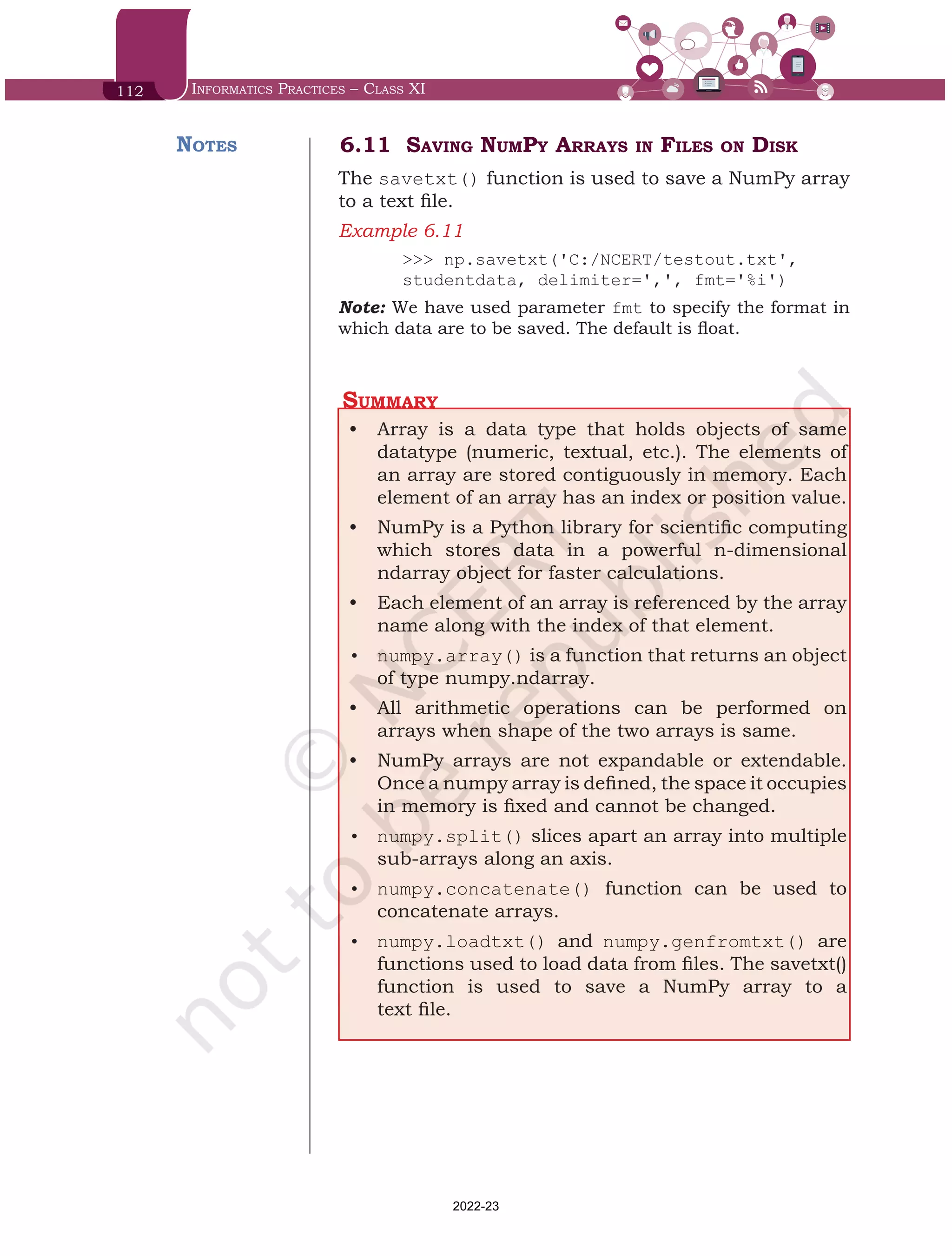
6.11 Saving NumPy Arrays in Files on Disk
The savetxt() function is used to save a NumPy array
to a text file.
Example 6.11
>>> np.savetxt('C:/NCERT/testout.txt',
studentdata, delimiter=',', fmt='%i')
Note: We have used parameter fmt to specify the format in
which data are to be saved. The default is float.
Summary
• Array is a data type that holds objects of same
datatype (numeric, textual, etc.). The elements of
an array are stored contiguously in memory. Each
element of an array has an index or position value.
• NumPy is a Python library for scientific computing
which stores data in a powerful n-dimensional
ndarray object for faster calculations.
• Each element of an array is referenced by the array
name along with the index of that element.
• numpy.array() is a function that returns an object
of type numpy.ndarray.
• All arithmetic operations can be performed on
arrays when shape of the two arrays is same.
• NumPy arrays are not expandable or extendable.
Once a numpy array is defined, the space it occupies
in memory is fixed and cannot be changed.
• numpy.split() slices apart an array into multiple
sub-arrays along an axis.
• numpy.concatenate() function can be used to
concatenate arrays.
• numpy.loadtxt() and numpy.genfromtxt() are
functions used to load data from files. The savetxt()
function is used to save a NumPy array to a
text file.
Notes
Chap 6.indd 112 19-Jul-19 3:43:32 PM
2022-23

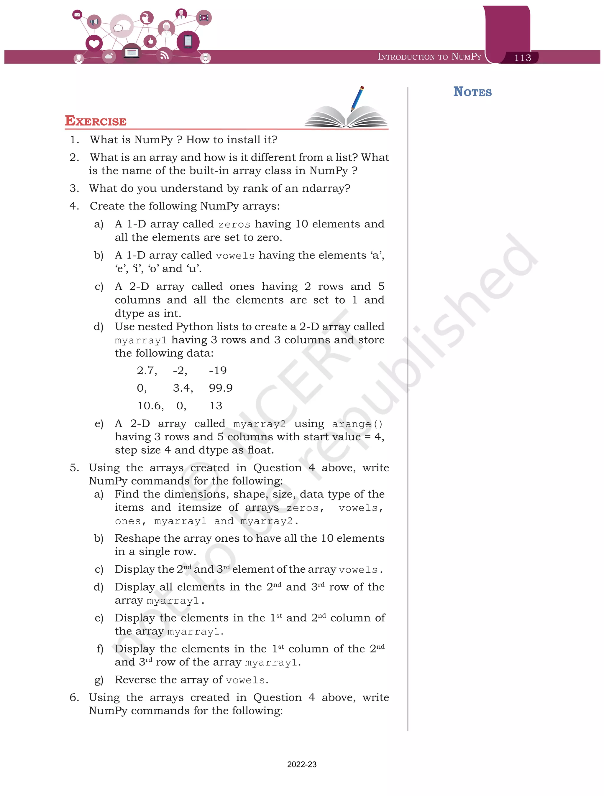
Exercise
1.
What is NumPy ? How to install it?
2. What is an array and how is it different from a list? What
is the name of the built-in array class in NumPy ?
3. What do you understand by rank of an ndarray?
4.
Create the following NumPy arrays:
a) A 1-D array called zeros having 10 elements and
all the elements are set to zero.
b) A 1-D array called vowels having the elements ‘a’,
‘e’, ‘i’, ‘o’ and ‘u’.
c) A 2-D array called ones having 2 rows and 5
columns and all the elements are set to 1 and
dtype as int.
d) Use nested Python lists to create a 2-D array called
myarray1 having 3 rows and 3 columns and store
the following data:
2.7, -2, -19
0, 3.4, 99.9
10.6, 0, 13
e) A 2-D array called myarray2 using arange()
having 3 rows and 5 columns with start value = 4,
step size 4 and dtype as float.
5. Using the arrays created in Question 4 above, write
NumPy commands for the following:
a) Find the dimensions, shape, size, data type of the
items and itemsize of arrays zeros, vowels,
ones, myarray1 and myarray2.
b) Reshape the array ones to have all the 10 elements
in a single row.
c) Display the 2nd
and 3rd
element of the array vowels.
d) Display all elements in the 2nd
and 3rd
row of the
array myarray1.
e) Display the elements in the 1st
and 2nd
column of
the array myarray1.
f) Display the elements in the 1st
column of the 2nd
and 3rd
row of the array myarray1.
g) Reverse the array of vowels.
6. Using the arrays created in Question 4 above, write
Notes
Chap 6.indd 113 19-Jul-19 3:43:33 PM
2022-23

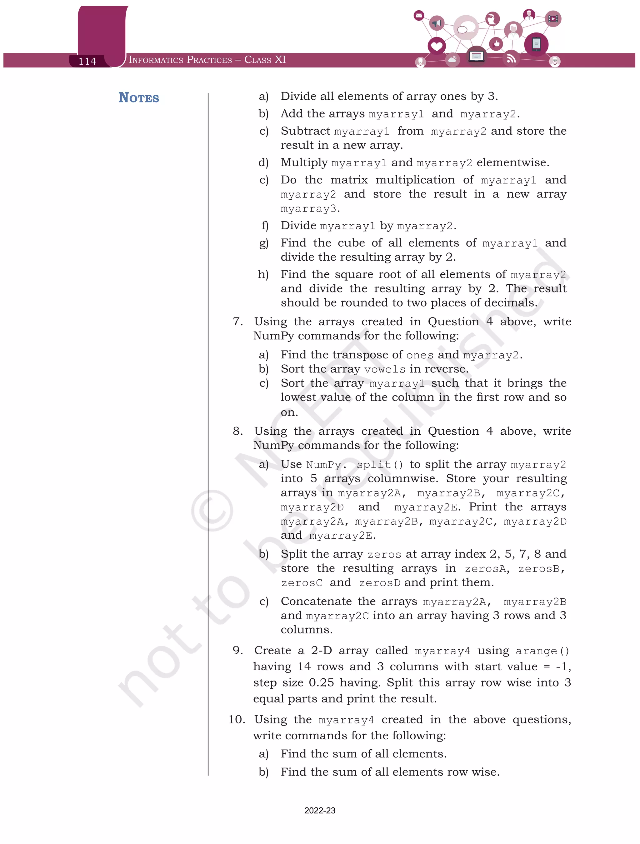
a) Divide all elements of array ones by 3.
b) Add the arrays myarray1 and myarray2.
c) Subtract myarray1 from myarray2 and store the
result in a new array.
d) Multiply myarray1 and myarray2 elementwise.
e) Do the matrix multiplication of myarray1 and
myarray2 and store the result in a new array
myarray3.
f) Divide myarray1 by myarray2.
g) Find the cube of all elements of myarray1 and
divide the resulting array by 2.
h) Find the square root of all elements of myarray2
and divide the resulting array by 2. The result
should be rounded to two places of decimals.
7.
Using the arrays created in Question 4 above, write
a) Find the transpose of ones and myarray2.
b) Sort the array vowels in reverse.
c) Sort the array myarray1 such that it brings the
lowest value of the column in the first row and so
on.
8.
Using the arrays created in Question 4 above, write
a) Use NumPy. split() to split the array myarray2
into 5 arrays columnwise. Store your resulting
arrays in myarray2A, myarray2B, myarray2C,
myarray2D and myarray2E. Print the arrays
myarray2A, myarray2B, myarray2C, myarray2D
and myarray2E.
b) Split the array zeros at array index 2, 5, 7, 8 and
store the resulting arrays in zerosA, zerosB,
zerosC and zerosD and print them.
c) Concatenate the arrays myarray2A, myarray2B
and myarray2C into an array having 3 rows and 3
columns.
9.
Create a 2-D array called myarray4 using arange()
having 14 rows and 3 columns with start value = -1,
step size 0.25 having. Split this array row wise into 3
equal parts and print the result.
10. Using the myarray4 created in the above questions,
write commands for the following:
a) Find the sum of all elements.
b) Find the sum of all elements row wise.
Notes
Chap 6.indd 114 19-Jul-19 3:43:33 PM
2022-23

Notes
c) Find the sum of all elements column wise.
d) Find the max of all elements.
e) Find the min of all elements in each row.
f) Find the mean of all elements in each row.
g) Find the standard deviation column wise.
Case Study (Solved)
We have already learnt that a data set (or dataset) is a
collection of data. Usually a data set corresponds to the
contents of a database table, or a statistical data matrix,
where every column of the table represents a particular
variable, and each row corresponds to a member or an item
etc. A data set lists values for each of the variables, such as
height and weight of a student, for each row (item) of the data
set. Open data refers to information released in a publicly
accessible repository.
The Iris flower data set is an example of an open data.
It is also called Fisher's Iris data set as this data set was
introduced by the British statistician and biologist Ronald
Fisher in 1936. The Iris data set consists of 50 samples from
each of the three species of the flower Iris (Iris setosa, Iris
virginica and Iris versicolor). Four features were measured
for each sample: the length and the width of the sepals and
petals, in centimeters. Based on the combination of these
four features, Fisher developed a model to distinguish one
species from each other. The full data set is freely available
on UCI Machine Learning Repository at https://archive.ics.
uci.edu/ml/datasets/iris.
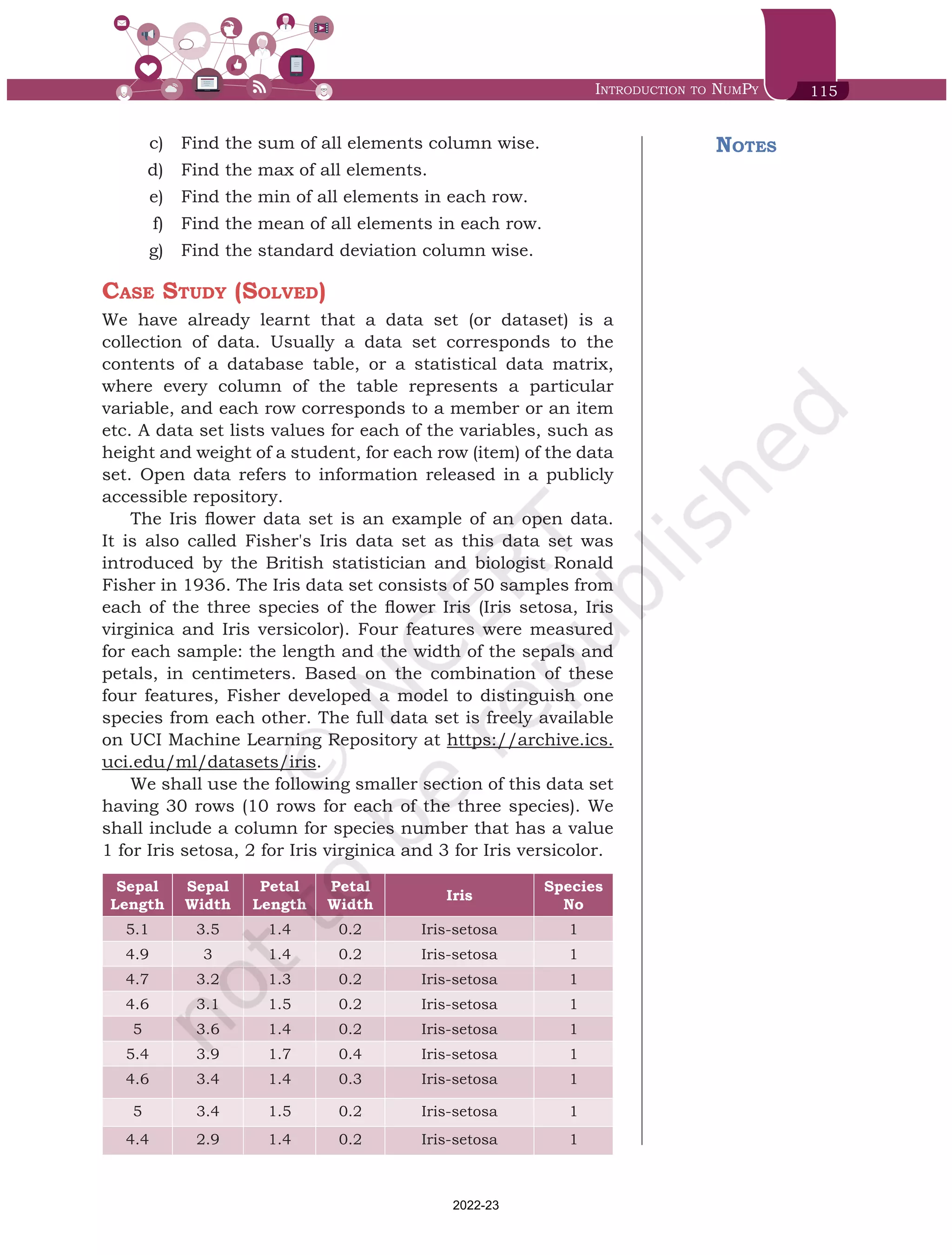
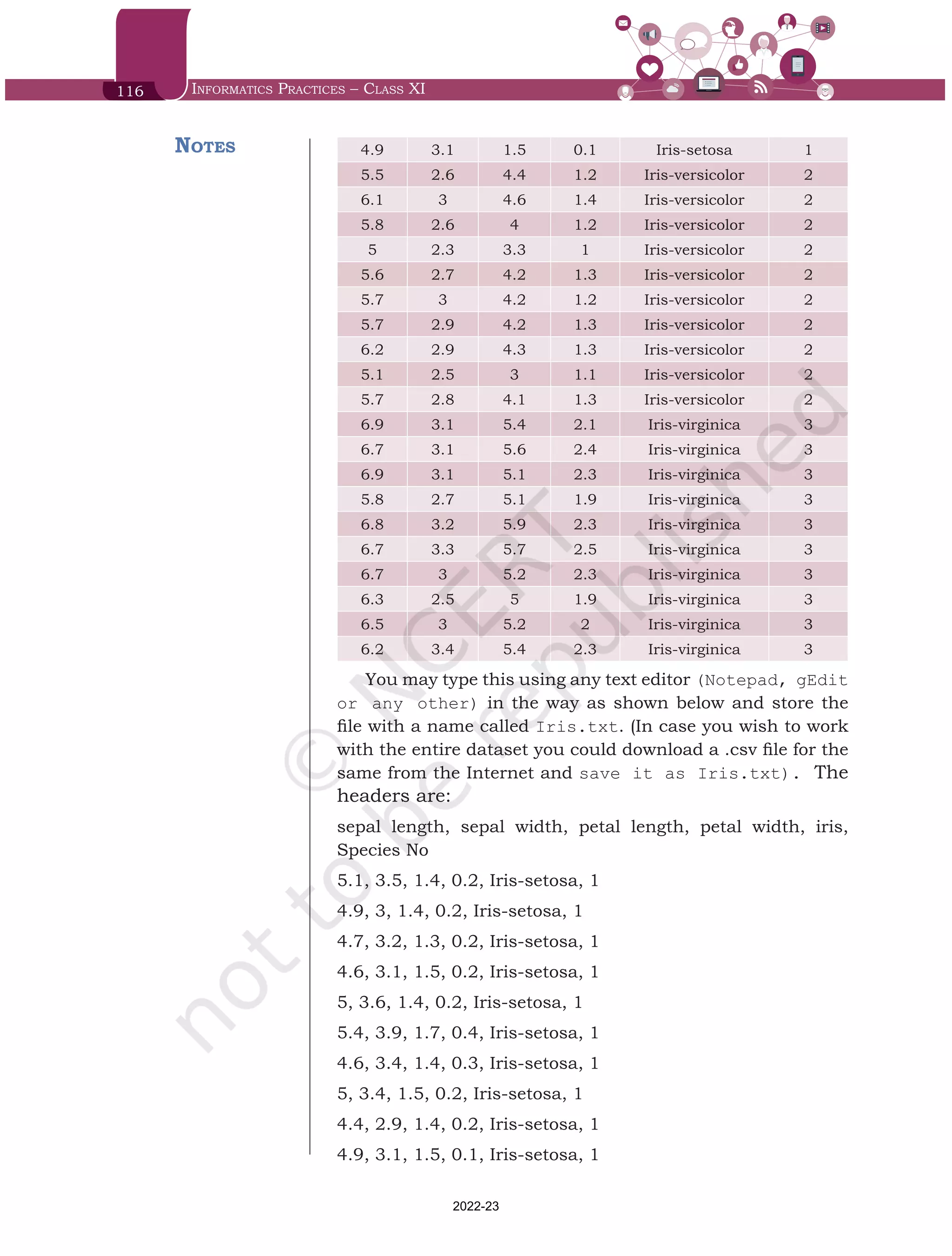
We shall use the following smaller section of this data set
having 30 rows (10 rows for each of the three species). We
shall include a column for species number that has a value
1 for Iris setosa, 2 for Iris virginica and 3 for Iris versicolor.
Sepal
Length
Sepal
Width
Petal
Length
Petal
Width
Iris
Species
No
5.1 3.5 1.4 0.2 Iris-setosa 1
4.9 3 1.4 0.2 Iris-setosa 1
4.7 3.2 1.3 0.2 Iris-setosa 1
4.6 3.1 1.5 0.2 Iris-setosa 1
5 3.6 1.4 0.2 Iris-setosa 1
5.4 3.9 1.7 0.4 Iris-setosa 1
4.6 3.4 1.4 0.3 Iris-setosa 1
5 3.4 1.5 0.2 Iris-setosa 1
4.4 2.9 1.4 0.2 Iris-setosa 1
Chap 6.indd 115 19-Jul-19 3:43:33 PM
2022-23

4.9 3.1 1.5 0.1 Iris-setosa 1
5.5 2.6 4.4 1.2 Iris-versicolor 2
6.1 3 4.6 1.4 Iris-versicolor 2
5.8 2.6 4 1.2 Iris-versicolor 2
5 2.3 3.3 1 Iris-versicolor 2
5.7 3 4.2 1.2 Iris-versicolor 2
5.1 2.5 3 1.1 Iris-versicolor 2
6.9 3.1 5.4 2.1 Iris-virginica 3
6.7 3 5.2 2.3 Iris-virginica 3
6.3 2.5 5 1.9 Iris-virginica 3
6.5 3 5.2 2 Iris-virginica 3
You may type this using any text editor (Notepad, gEdit
or any other) in the way as shown below and store the
file with a name called Iris.txt. (In case you wish to work
with the entire dataset you could download a .csv file for the
same from the Internet and save it as Iris.txt). The
headers are:
sepal length, sepal width, petal length, petal width, iris,
Species No
5.1, 3.5, 1.4, 0.2, Iris-setosa, 1
4.9, 3, 1.4, 0.2, Iris-setosa, 1
4.7, 3.2, 1.3, 0.2, Iris-setosa, 1
4.6, 3.1, 1.5, 0.2, Iris-setosa, 1
5, 3.6, 1.4, 0.2, Iris-setosa, 1
5.4, 3.9, 1.7, 0.4, Iris-setosa, 1
4.6, 3.4, 1.4, 0.3, Iris-setosa, 1
5, 3.4, 1.5, 0.2, Iris-setosa, 1
4.4, 2.9, 1.4, 0.2, Iris-setosa, 1
4.9, 3.1, 1.5, 0.1, Iris-setosa, 1
Notes
Chap 6.indd 116 19-Jul-19 3:43:33 PM
2022-23

5.5, 2.6, 4.4, 1.2, Iris-versicolor, 2
6.1, 3, 4.6, 1.4, Iris-versicolor, 2
5.8, 2.6, 4, 1.2, Iris-versicolor, 2
5, 2.3, 3.3, 1, Iris-versicolor, 2
5.6, 2.7, 4.2, 1.3, Iris-versicolor, 2
5.7, 3, 4.2, 1.2, Iris-versicolor, 2
5.7, 2.9, 4.2, 1.3, Iris-versicolor, 2
6.2, 2.9, 4.3, 1.3, Iris-versicolor, 2
5.1, 2.5, 3, 1.1, Iris-versicolor, 2
5.7, 2.8, 4.1, 1.3, Iris-versicolor, 2
6.9, 3.1, 5.4, 2.1, Iris-virginica, 3
6.7, 3.1, 5.6, 2.4, Iris-virginica, 3
6.9, 3.1, 5.1, 2.3, Iris-virginica, 3
5.8, 2.7, 5.1, 1.9, Iris-virginica, 3
6.8, 3.2, 5.9, 2.3, Iris-virginica, 3
6.7, 3.3, 5.7, 2.5, Iris-virginica, 3
6.7, 3, 5.2, 2.3, Iris-virginica, 3
6.3, 2.5, 5, 1.9, Iris-virginica, 3
6.5, 3, 5.2, 2, Iris-virginica, 3
6.2, 3.4, 5.4, 2.3, Iris-virginica, 3
1. Load the data in the file Iris.txt in a 2-D array called
iris.
2.
Drop column whose index = 4 from the array iris.
3.
Display the shape, dimensions and size of iris.
4. Split iris into three 2-D arrays, each array for a different
species. Call them iris1, iris2, iris3.
5.
Print the three arrays iris1, iris2, iris3
6.
Create a 1-D array header having elements "sepal
length", "sepal width", "petal length", "petal width",
"Species No" in that order.
7.
Display the array header.
8. Find the max, min, mean and standard deviation for the
columns of the iris and store the results in the arrays
iris_max, iris_min, iris_avg, iris_std, iris_
var respectively. The results must be rounded to not
more than two decimal places.
Notes
Chap 6.indd 117 19-Jul-19 3:43:33 PM
2022-23

9.
Similarly find the max, min, mean and standard deviation
for the columns of the iris1, iris2 and iris3 and
store the results in the arrays with appropriate names.
10.
Check the minimum value for sepal length, sepal width,
petal length and petal width of the three species in
comparison to the minimum value of sepal length, sepal
width, petal length and petal width for the data set as a
whole and fill the table below with True if the species value
is greater than the dataset value and False otherwise.
Iris setosa Iris virginica Iris versicolor
sepal length
sepal width
petal length
petal width
11.
Compare Iris setosa’s average sepal width to that of Iris
virginica.
12.
Compare Iris setosa’s average petal length to that of Iris
virginica.
13.
Compare Iris setosa’s average petal width to that of Iris
virginica.
14.
Save the array iris_avg in a comma separated file
named IrisMeanValues.txt on the hard disk.
15.
Save the arrays iris_max, iris_avg, iris_min in
a comma separated file named IrisStat.txt on the
hard disk.
Solutions to Case Study based Exercises
>>> import numpy as np
# Solution to Q1
>>> iris = np.genfromtxt('C:/NCERT/Iris.txt',skip_
header=1, delimiter=',', dtype = float)
# Solution to Q2
>>> iris = iris[0:30,[0,1,2,3,5]] # drop column 4
# Solution to Q3
>>> iris.shape
(30, 5)
>>> iris.ndim
Notes
Chap 6.indd 118 19-Jul-19 3:43:33 PM
2022-23

2
>>> iris.size
150
# Solution to Q4
# Split into three arrays, each array for a different
# species
>>> iris1, iris2, iris3 = np.split(iris, [10,20],
axis=0)
# Solution to Q5
# Print the three arrays
>>> iris1
array([[5.1, 3.5, 1.4, 0.2, 1. ],
[4.9, 3. , 1.4, 0.2, 1. ],
[4.7, 3.2, 1.3, 0.2, 1. ],
[4.6, 3.1, 1.5, 0.2, 1. ],
[5. , 3.6, 1.4, 0.2, 1. ],
[5.4, 3.9, 1.7, 0.4, 1. ],
[4.6, 3.4, 1.4, 0.3, 1. ],
[5. , 3.4, 1.5, 0.2, 1. ],
[4.4, 2.9, 1.4, 0.2, 1. ],
[4.9, 3.1, 1.5, 0.1, 1. ]])
>>> iris2
array([[5.5, 2.6, 4.4, 1.2, 2. ],
[6.1, 3. , 4.6, 1.4, 2. ],
[5.8, 2.6, 4. , 1.2, 2. ],
[5. , 2.3, 3.3, 1. , 2. ],
[5.6, 2.7, 4.2, 1.3, 2. ],
[5.7, 3. , 4.2, 1.2, 2. ],
[5.7, 2.9, 4.2, 1.3, 2. ],
[6.2, 2.9, 4.3, 1.3, 2. ],
[5.1, 2.5, 3. , 1.1, 2. ],
[5.7, 2.8, 4.1, 1.3, 2. ]])
>>> iris3
array([[6.9, 3.1, 5.4, 2.1, 3. ],
[6.7, 3.1, 5.6, 2.4, 3. ],
[6.9, 3.1, 5.1, 2.3, 3. ],
[5.8, 2.7, 5.1, 1.9, 3. ],
[6.8, 3.2, 5.9, 2.3, 3. ],
[6.7, 3.3, 5.7, 2.5, 3. ],
[6.7, 3. , 5.2, 2.3, 3. ],
[6.3, 2.5, 5. , 1.9, 3. ],
[6.5, 3. , 5.2, 2. , 3. ],
[6.2, 3.4, 5.4, 2.3, 3. ]])
Notes
Chap 6.indd 119 19-Jul-19 3:43:33 PM
2022-23

# Solution to Q6
>>> header =np.array(["sepal length", "sepal
width", "petal length", "petal width",
"Species No"])
# Solution to Q7
>>> print(header)
['sepal length' 'sepal width' 'petal length' 'petal
width' 'Species No']
# Solution to Q8
# Stats for array iris
# Finds the max of the data for sepal length, sepal
width, petal length, petal width, Species No
>>> iris_max = iris.max(axis=0)
>>> iris_max
array([6.9, 3.9, 5.9, 2.5, 3. ])
# Finds the min of the data for sepal length, sepal
# width, petal length, petal width, Species No
>>> iris_min = iris.min(axis=0)
>>> iris_min
array([4.4, 2.3, 1.3, 0.1, 1. ])
# Finds the mean of the data for sepal length, sepal
# width, petal length, petal width, Species No
>>> iris_avg = iris.mean(axis=0).round(2)
>>> iris_avg
array([5.68, 3.03, 3.61, 1.22, 2. ])
# Finds the standard deviation of the data for sepal
# length, sepal width, petal length, petal width,
# Species No
>>> iris_std = iris.std(axis=0).round(2)
>>> iris_std
array([0.76, 0.35, 1.65, 0.82, 0.82])
# Solution to Q9
>>> iris1_max = iris1.max(axis=0)
>>> iris1_max
array([5.4, 3.9, 1.7, 0.4, 1. ])
>>> iris2_max
array([6.2, 3. , 4.6, 1.4, 2. ])
Notes
Chap 6.indd 120 19-Jul-19 3:43:33 PM
2022-23

>>> iris3_max
array([6.9, 3.4, 5.9, 2.5, 3. ])
>>> iris1_min = iris1.min(axis=0)
>>> iris1_min
array([4.4, 2.9, 1.3, 0.1, 1. ])
>>> iris2_min
array([5. , 2.3, 3. , 1. , 2. ])
>>> iris3_min
array([5.8, 2.5, 5. , 1.9, 3. ])
>>> iris1_avg = iris1.mean(axis=0)
>>> iris1_avg
array([4.86, 3.31, 1.45, 0.22, 1. ])
>>> iris2_avg
array([5.64, 2.73, 4.03, 1.23, 2. ])
>>> iris3_avg
array([6.55, 3.04, 5.36, 2.2 , 3. ])
>>> iris1_std = iris1.std(axis=0).round(2)
>>> iris1_std
array([0.28, 0.29, 0.1 , 0.07, 0. ])
>>> iris2_std
array([0.36, 0.22, 0.47, 0.11, 0. ])
>>> iris3_std
array([0.34, 0.25, 0.28, 0.2 , 0. ])
# Solution to Q10 (solve other parts on the same lines)
# min sepal length of each species Vs the min sepal
# length in the data set
>>> iris1_min[0] > iris_min[0] #sepal length
False
Notes
Chap 6.indd 121 19-Jul-19 3:43:33 PM
2022-23

>>> iris2_min[0] > iris_min[0]
True
>>> iris3_min[0] > iris_min[0]
True
# Solution to Q11
#Compare Iris setosa and Iris virginica
>>> iris1_avg[1] > iris2_avg[1] #sepal width
True
# Solution to Q12
>>> iris1_avg[2] > iris2_avg[2] #petal length
False
# Solution to Q13
>>> iris1_avg[3] > iris2_avg[3] #petal width
False
# Solution to Q14
>>> np.savetxt('C:/NCERT/IrisMeanValues.txt',
iris_avg, delimiter = ',')
# Solution to Q15
>>> np.savetxt('C:/NCERT/IrisStat.txt', (iris_
max, iris_avg, iris_min), delimiter=',')
Notes
Chap 6.indd 122 19-Jul-19 3:43:33 PM
2022-23

numpy.pdf

Recommended

Recommended

More Related Content

Similar to numpy.pdf

Similar to numpy.pdf (20)

Recently uploaded

Recently uploaded (20)

numpy.pdf