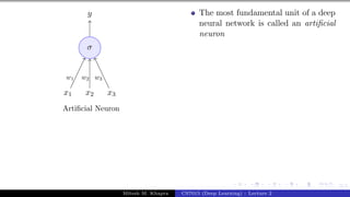
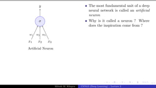
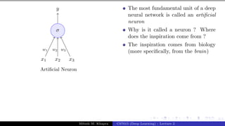
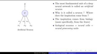
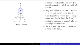
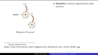
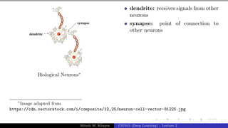
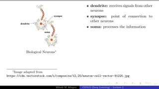
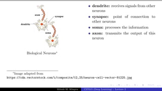
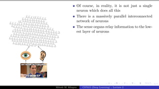
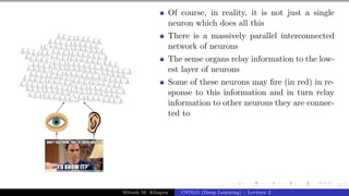
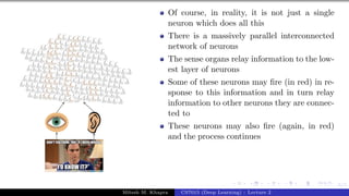
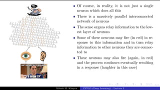
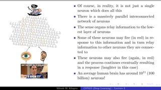
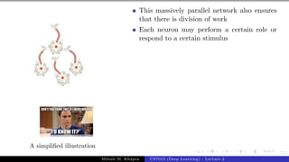
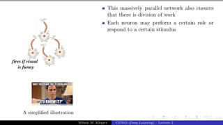
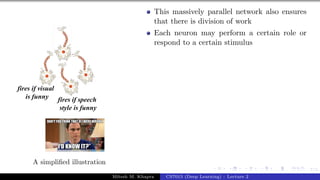
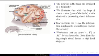
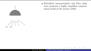
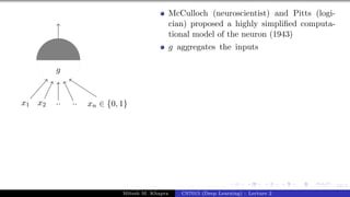
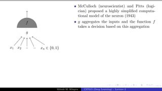
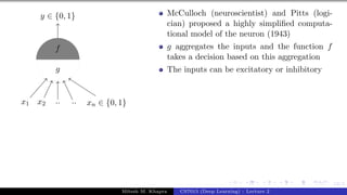
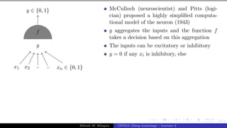
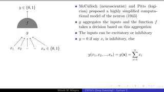
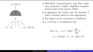
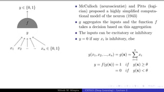
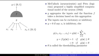
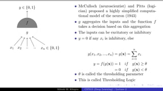
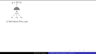
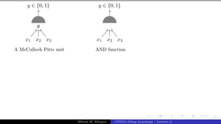
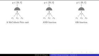
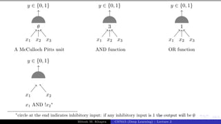
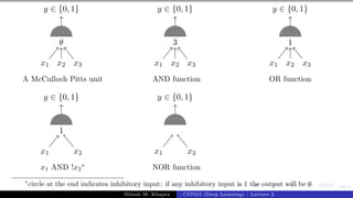
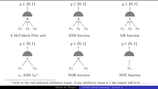
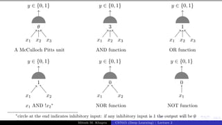
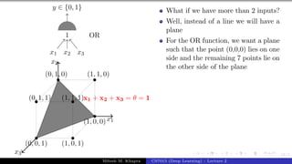
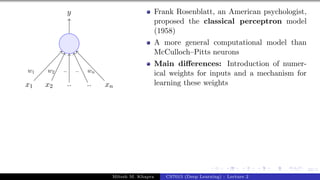
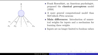
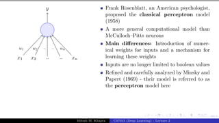
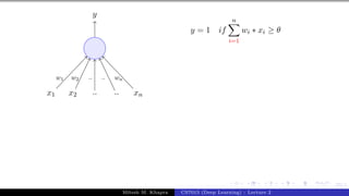
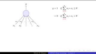
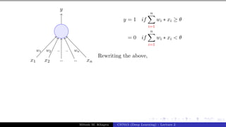
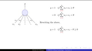
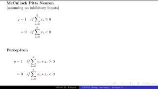
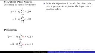
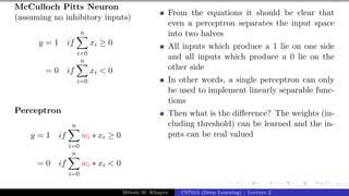
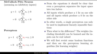
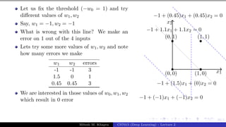
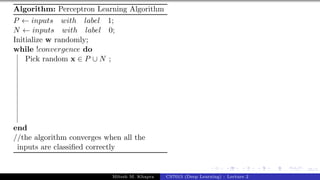
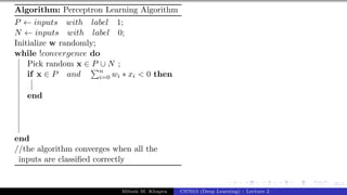
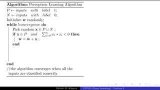
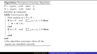
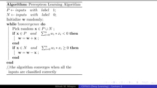
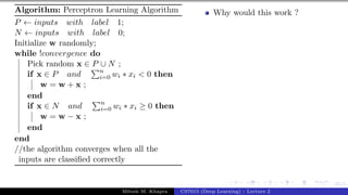
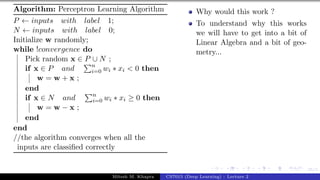
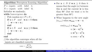
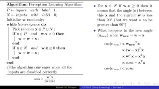
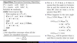
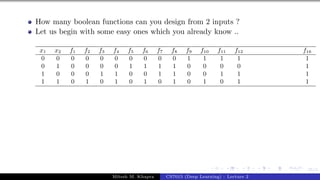
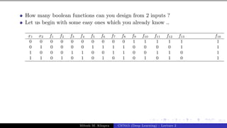
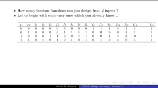
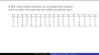
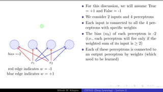
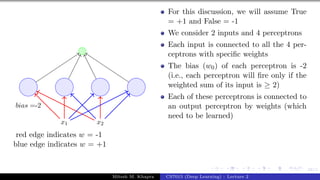
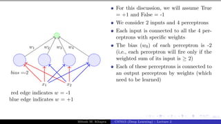
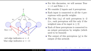
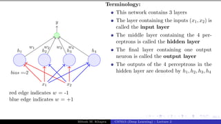
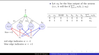
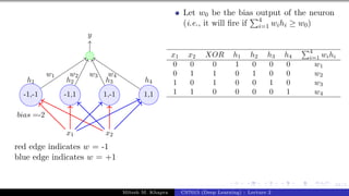
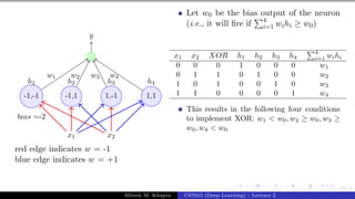
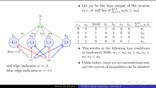
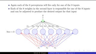
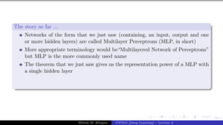
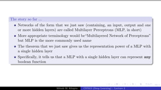
The document describes a lecture on deep learning. It begins by discussing biological neurons and how they inspired artificial neurons. The McCulloch-Pitts neuron is then introduced as a simplified computational model of a neuron. The model defines a neuron as having binary inputs that are aggregated and passed through an activation function to produce a binary output. The lecture also covers topics like threshold logic, perceptrons, multilayer perceptrons, and the hierarchical arrangement of neurons in the brain.


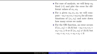
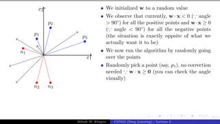
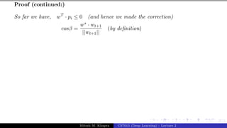
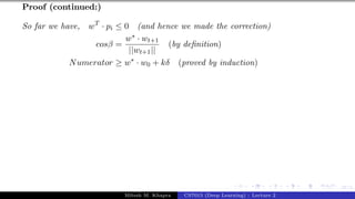
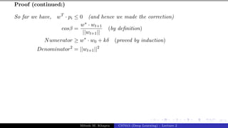
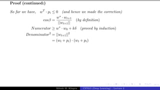
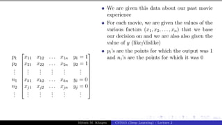
![25/1
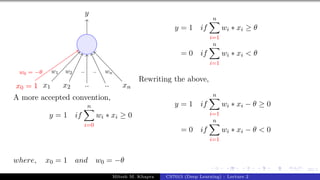
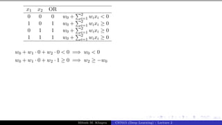
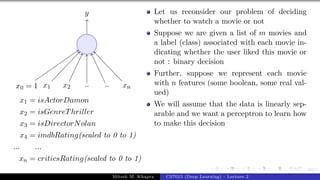
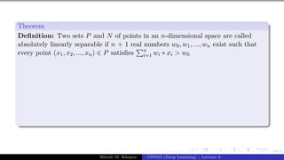
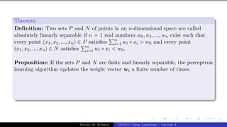
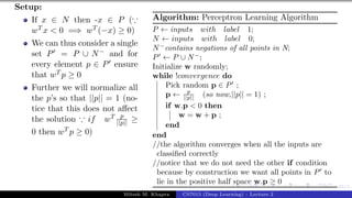
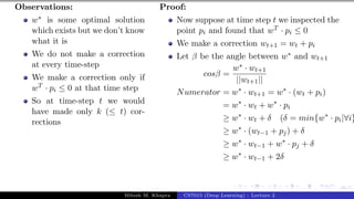
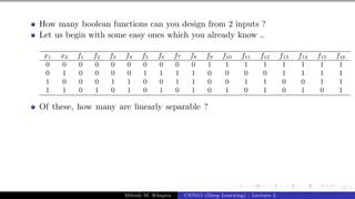
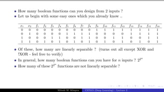
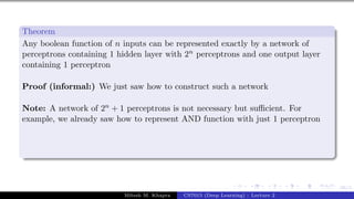
x0 = 1 x1 x2 x3
y
w0 = −θ w1 w2 w3
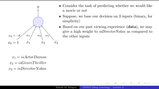
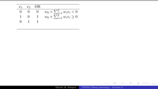
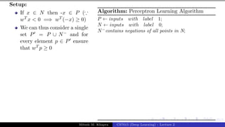
x1 = isActorDamon
x2 = isGenreThriller
x3 = isDirectorNolan
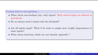
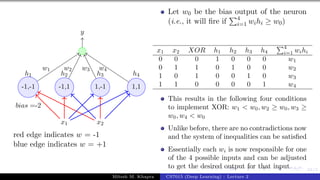
w0 is called the bias as it represents the prior (preju-
dice)
A movie buff may have a very low threshold and may
watch any movie irrespective of the genre, actor, dir-
ector [θ = 0]
Mitesh M. Khapra CS7015 (Deep Learning) : Lecture 2](https://image.slidesharecdn.com/lecture2-240214132905-7cd361d0/85/NPTEL-Deep-Learning-Lecture-notes-for-session-2-119-320.jpg)
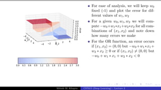
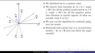
![25/1
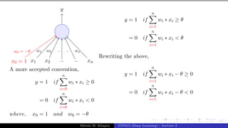
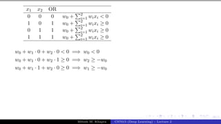
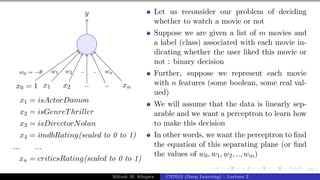
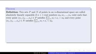
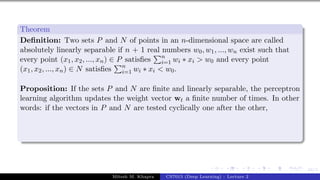
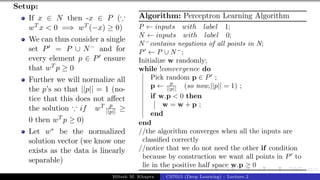
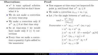
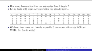
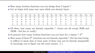
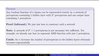
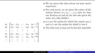
x0 = 1 x1 x2 x3
y
w0 = −θ w1 w2 w3
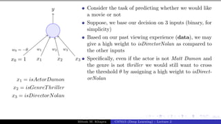
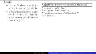
x1 = isActorDamon
x2 = isGenreThriller
x3 = isDirectorNolan
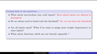
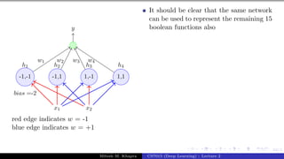
w0 is called the bias as it represents the prior (preju-
dice)
A movie buff may have a very low threshold and may
watch any movie irrespective of the genre, actor, dir-
ector [θ = 0]
On the other hand, a selective viewer may only watch
thrillers starring Matt Damon and directed by Nolan
[θ = 3]
Mitesh M. Khapra CS7015 (Deep Learning) : Lecture 2](https://image.slidesharecdn.com/lecture2-240214132905-7cd361d0/85/NPTEL-Deep-Learning-Lecture-notes-for-session-2-120-320.jpg)
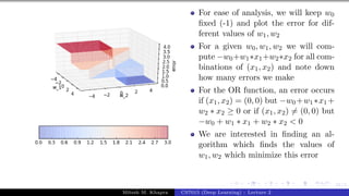
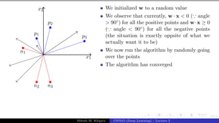
![25/1
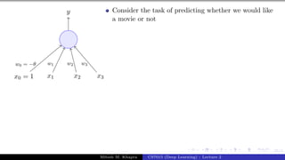
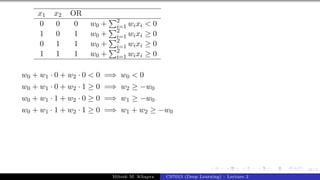
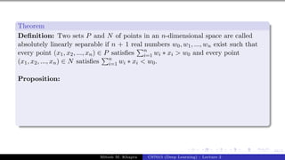
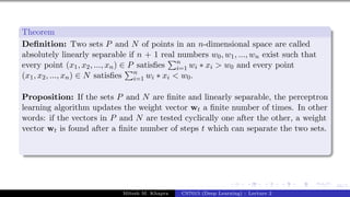
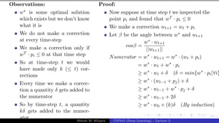
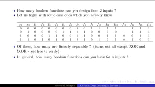
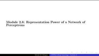
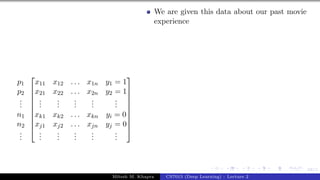
x0 = 1 x1 x2 x3
y
w0 = −θ w1 w2 w3
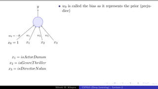
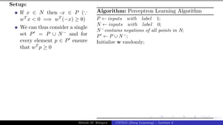
x1 = isActorDamon
x2 = isGenreThriller
x3 = isDirectorNolan
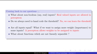
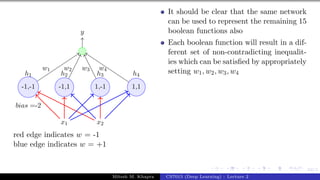
w0 is called the bias as it represents the prior (preju-
dice)
A movie buff may have a very low threshold and may
watch any movie irrespective of the genre, actor, dir-
ector [θ = 0]
On the other hand, a selective viewer may only watch
thrillers starring Matt Damon and directed by Nolan
[θ = 3]
The weights (w1, w2, ..., wn) and the bias (w0) will de-
pend on the data (viewer history in this case)
Mitesh M. Khapra CS7015 (Deep Learning) : Lecture 2](https://image.slidesharecdn.com/lecture2-240214132905-7cd361d0/85/NPTEL-Deep-Learning-Lecture-notes-for-session-2-121-320.jpg)


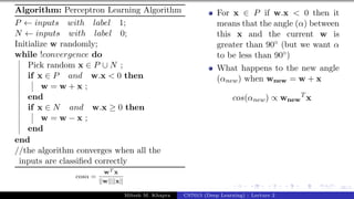
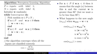
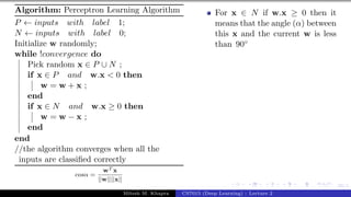
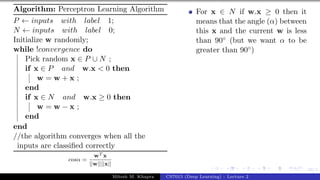
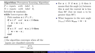
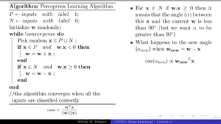
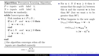
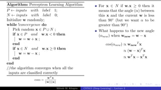
![36/1
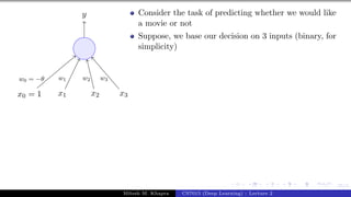
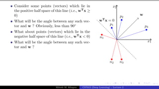
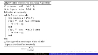
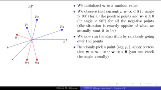
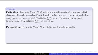
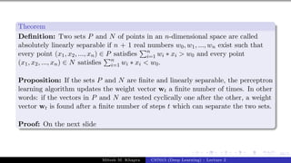
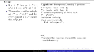
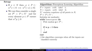
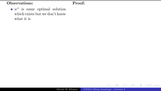
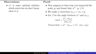
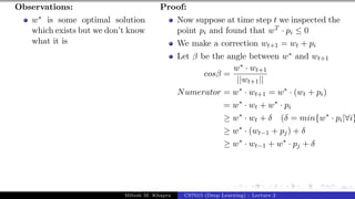
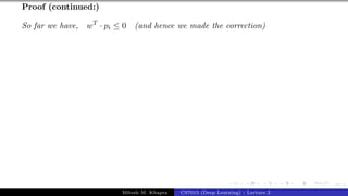
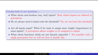
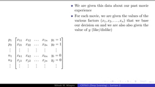
Consider two vectors w and x
w = [w0, w1, w2, ..., wn]
x = [1, x1, x2, ..., xn]
Mitesh M. Khapra CS7015 (Deep Learning) : Lecture 2](https://image.slidesharecdn.com/lecture2-240214132905-7cd361d0/85/NPTEL-Deep-Learning-Lecture-notes-for-session-2-188-320.jpg)
![36/1
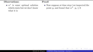
Consider two vectors w and x
w = [w0, w1, w2, ..., wn]
x = [1, x1, x2, ..., xn]
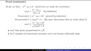
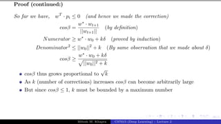
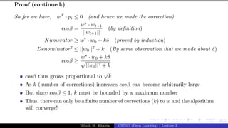
w · x = wT
x =
n
X
i=0
wi ∗ xi
Mitesh M. Khapra CS7015 (Deep Learning) : Lecture 2](https://image.slidesharecdn.com/lecture2-240214132905-7cd361d0/85/NPTEL-Deep-Learning-Lecture-notes-for-session-2-189-320.jpg)
![36/1
Consider two vectors w and x
w = [w0, w1, w2, ..., wn]
x = [1, x1, x2, ..., xn]
w · x = wT
x =
n
X
i=0
wi ∗ xi
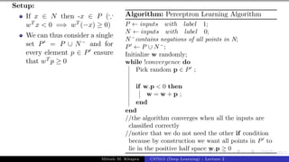
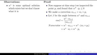
We can thus rewrite the perceptron
rule as
Mitesh M. Khapra CS7015 (Deep Learning) : Lecture 2](https://image.slidesharecdn.com/lecture2-240214132905-7cd361d0/85/NPTEL-Deep-Learning-Lecture-notes-for-session-2-190-320.jpg)
![36/1
Consider two vectors w and x
w = [w0, w1, w2, ..., wn]
x = [1, x1, x2, ..., xn]
w · x = wT
x =
n
X
i=0
wi ∗ xi
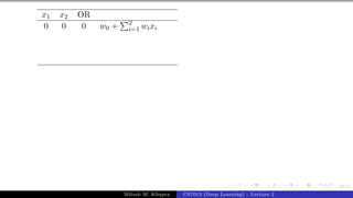
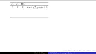
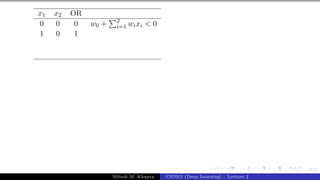
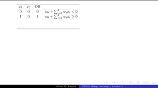
We can thus rewrite the perceptron
rule as
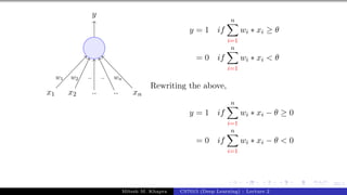
y = 1 if wT
x ≥ 0
= 0 if wT
x < 0
Mitesh M. Khapra CS7015 (Deep Learning) : Lecture 2](https://image.slidesharecdn.com/lecture2-240214132905-7cd361d0/85/NPTEL-Deep-Learning-Lecture-notes-for-session-2-191-320.jpg)
![36/1
Consider two vectors w and x
w = [w0, w1, w2, ..., wn]
x = [1, x1, x2, ..., xn]
w · x = wT
x =
n
X
i=0
wi ∗ xi
We can thus rewrite the perceptron
rule as
y = 1 if wT
x ≥ 0
= 0 if wT
x < 0
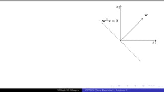
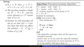
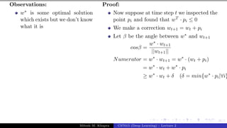
We are interested in finding the line
wTx = 0 which divides the input
space into two halves
Mitesh M. Khapra CS7015 (Deep Learning) : Lecture 2](https://image.slidesharecdn.com/lecture2-240214132905-7cd361d0/85/NPTEL-Deep-Learning-Lecture-notes-for-session-2-192-320.jpg)
![36/1
Consider two vectors w and x
w = [w0, w1, w2, ..., wn]
x = [1, x1, x2, ..., xn]
w · x = wT
x =
n
X
i=0
wi ∗ xi
We can thus rewrite the perceptron
rule as
y = 1 if wT
x ≥ 0
= 0 if wT
x < 0
We are interested in finding the line
wTx = 0 which divides the input
space into two halves
Every point (x) on this line satisfies
the equation wTx = 0
Mitesh M. Khapra CS7015 (Deep Learning) : Lecture 2](https://image.slidesharecdn.com/lecture2-240214132905-7cd361d0/85/NPTEL-Deep-Learning-Lecture-notes-for-session-2-193-320.jpg)
![36/1
Consider two vectors w and x
w = [w0, w1, w2, ..., wn]
x = [1, x1, x2, ..., xn]
w · x = wT
x =
n
X
i=0
wi ∗ xi
We can thus rewrite the perceptron
rule as
y = 1 if wT
x ≥ 0
= 0 if wT
x < 0
We are interested in finding the line
wTx = 0 which divides the input
space into two halves
Every point (x) on this line satisfies
the equation wTx = 0
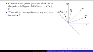
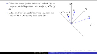
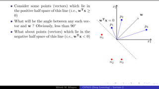
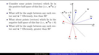
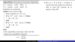
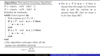
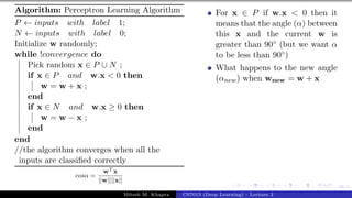
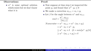
What can you tell about the angle (α)
between w and any point (x) which
lies on this line ?
Mitesh M. Khapra CS7015 (Deep Learning) : Lecture 2](https://image.slidesharecdn.com/lecture2-240214132905-7cd361d0/85/NPTEL-Deep-Learning-Lecture-notes-for-session-2-194-320.jpg)
![36/1
Consider two vectors w and x
w = [w0, w1, w2, ..., wn]
x = [1, x1, x2, ..., xn]
w · x = wT
x =
n
X
i=0
wi ∗ xi
We can thus rewrite the perceptron
rule as
y = 1 if wT
x ≥ 0
= 0 if wT
x < 0
We are interested in finding the line
wTx = 0 which divides the input
space into two halves
Every point (x) on this line satisfies
the equation wTx = 0
What can you tell about the angle (α)
between w and any point (x) which
lies on this line ?
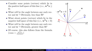
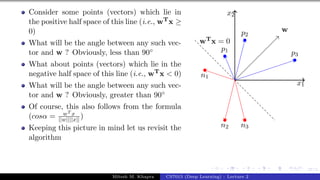
The angle is 90◦ (∵ cosα = wT x
||w||||x|| =
0)
Mitesh M. Khapra CS7015 (Deep Learning) : Lecture 2](https://image.slidesharecdn.com/lecture2-240214132905-7cd361d0/85/NPTEL-Deep-Learning-Lecture-notes-for-session-2-195-320.jpg)
![36/1
Consider two vectors w and x
w = [w0, w1, w2, ..., wn]
x = [1, x1, x2, ..., xn]
w · x = wT
x =
n
X
i=0
wi ∗ xi
We can thus rewrite the perceptron
rule as
y = 1 if wT
x ≥ 0
= 0 if wT
x < 0
We are interested in finding the line
wTx = 0 which divides the input
space into two halves
Every point (x) on this line satisfies
the equation wTx = 0
What can you tell about the angle (α)
between w and any point (x) which
lies on this line ?
The angle is 90◦ (∵ cosα = wT x
||w||||x|| =
0)
Since the vector w is perpendicular to
every point on the line it is actually
perpendicular to the line itself
Mitesh M. Khapra CS7015 (Deep Learning) : Lecture 2](https://image.slidesharecdn.com/lecture2-240214132905-7cd361d0/85/NPTEL-Deep-Learning-Lecture-notes-for-session-2-196-320.jpg)


![Presentation on b trees [autosaved]](https://cdn.slidesharecdn.com/ss_thumbnails/presentationonbtreesautosaved-210209155822-thumbnail.jpg?width=640&height=640&fit=bounds)


