Machine Learning
By
Dr.G.MADHU
M.Tech., Ph.D., MIEEE., MCSI., MISTE., MISRS., MIRSS., MIAENG
Professor,
Department of Information Technology,
VNR Vignana Jyothi Institute of Engineering & Technology,
Bachupally, Nizampet (S.O.)
Hyderabad- 500 090,RangaReddy Dt. TELANGANA, INDIA.
Cell: +919849085728
E-mail: madhu_g@vnrvjiet.in
Subject Code: 22PC1IT302
Unit-5: Artificial Neural Networks
Machine Learning Course- Dr G Madhu 2
4/28/2025
• “Artificial Neural Networks or ANN is an
information processing paradigm that is inspired
by the way the biological nervous system such as
brain process information.
• It is composed of large number of highly
interconnected processing elements (neurons)
working in unison to solve a specific problem.”
• The brain is a highly complex, nonlinear, and
parallel computer (information-processing
system).
Machine Learning Course- Dr G Madhu 3
Introduction to Artificial Neural Networks
4/28/2025
• Brain has the capability to organize its structural
constituents, known as neurons, so as to
perform certain computations (e.g., pattern
recognition, perception, and motor control)
many times faster than the fastest digital
computer in existence today.
• Consider, for example, human vision, which is
an information-processing task.
• It is the function of the visual system to provide
a representation of the environment around us
and, more important, to supply the information
we need to interact with the environment.
Machine Learning Course- Dr G Madhu 4
4/28/2025
• To be specific, the brain routinely
accomplishes perceptual recognition tasks
(e.g., recognizing a familiar face embedded in
an unfamiliar scene) in approximately
100–200 ms, whereas tasks of much lesser
complexity take a great deal longer on a
powerful computer.
4/28/2025 Machine Learning Course- Dr G Madhu 5
4/28/2025 Machine Learning Course- Dr G Madhu 6
• Although artificial neurons and perceptrons
were inspired by the biological processes
scientists were able to observe in the brain
back in the 50s, they do differ from their
biological counterparts in several ways.
• Birds have inspired flight and horses have
inspired locomotives and cars, yet none of
today’s transportation vehicles resemble metal
skeletons of living-breathing-self replicating
animals.
• Def: A neural network is a massively parallel
distributed processor made up of simple
processing units that has a natural propensity
for storing experiential knowledge and making
it available for use.
• It resembles the brain in two respects:
1. Knowledge is acquired by the network from its
environment through a learning process.
2. Inter-neuron connection strengths, known as
synaptic weights, are used to store the acquired
knowledge.
4/28/2025 Machine Learning Course- Dr G Madhu 7
• The procedure used to perform the learning
process is called a learning algorithm
Biological Neural Networks
• A biological neural network is composed of a
groups of chemically connected or functionally
associated neurons.
4/28/2025 Machine Learning Course- Dr G Madhu 8
4/28/2025 Machine Learning Course- Dr G Madhu 9
https://en.wikipedia.org/wiki/Artificial_neural_network#/media/File:Neuron3.png
• The human nervous system contains cells, which
are referred to as neurons.
• The neurons are connected to one another with
the use of axons and dendrites, and the
connecting regions between axons and dendrites
are referred to as synapses.
• Tree like nerve fibres called dendrites are
associated with the cell body.
• These dendrites receive signals from other
neurons.
4/28/2025 Machine Learning Course- Dr G Madhu 10
4/28/2025 Machine Learning Course- Dr G Madhu 11
4/28/2025 Machine Learning Course- Dr G Madhu 12
4/28/2025 Machine Learning Course- Dr G Madhu 13
Source: https://www.kaggle.com/androbomb/simple-nn-with-python-multi-layer-perceptron
• These dendrites receive signals from other
neurons.
• Extending from the cell body is a single long
fibre called the axon, which eventually
branches into strands and substrands
connecting to many other neurons at the
synaptic junctions, or synapses.
4/28/2025 Machine Learning Course- Dr G Madhu 14
Basic Notations
4/28/2025
1. Dendrite
– Dendrites are responsible for getting
incoming signals from outside
2. Soma
– Soma is the cell body responsible for
the processing of input signals and
deciding whether a neuron should
fire an output signal
3. Axon
– Axon is responsible for getting
processed signals from neuron to
relevant cells
4. Synapse
– Synapse is the connection between
an axon and other neuron dendrites
Machine Learning Course- Dr G Madhu 15
What is Artificial
Neuron?
• An artificial neuron is a mathematical function
conceived as a model of biological neurons, a
neural network.
• Artificial neurons are elementary units in an
artificial neural network.
4/28/2025 Machine Learning Course- Dr G Madhu 16
4/28/2025 Machine Learning Course- Dr G Madhu 17
illustration of a single biological neuron annotated to describe a single artificial neurons
function.
4/28/2025 Machine Learning Course- Dr G Madhu 18
• A biological neuron receives input signals
from its dendrites from other neurons and
sends output signals along its axon, which
branches out and connects to other neurons.
• In the illustration above, the input signal is
represented by x0
, as this signal ‘travels’ it is
multiplied (w0
x0
) based on the a weight
variable (w0
).
• The weight variables are learnable and the
weights strength and polarity (positive or
negative) control the influence of the signal.
4/28/2025 Machine Learning Course- Dr G Madhu 19
• The influence is determined by summing the
signal input and weight (∑wi
xi
+ b) which is
then calculated by the activation function f, if
it is above a certain threshold the neuron
fires.
4/28/2025 Machine Learning Course- Dr G Madhu 20
Artificial Neurons
• Artificial neuron also known as perceptron is
the basic unit of the neural network.
• In simple terms, it is a mathematical function
based on a model of biological neurons.
or
A neuron is an information-processing unit that is
fundamental to the operation of a neural
network
4/28/2025 Machine Learning Course- Dr G Madhu 21
What is Artificial Neural Network (ANN)?
• The human brain is considered the most
complicated object in the universe.
• Artificial Neural Network (ANN), which is a
system of computing that is loosely modelled on
the structure of the brain.
4/28/2025 Machine Learning Course- Dr G Madhu 22
The Block Diagram of Model of a Neuron
4/28/2025 Machine Learning Course- Dr G Madhu 23
Fig.1. Nonlinear model of a neuron, labelled k.
• In mathematical terms, we may describe the
neuron k depicted in above Fig.1 by writing
the pair of equations:
4/28/2025 Machine Learning Course- Dr G Madhu 24
• The use of bias bk
has the effect of applying an affine
transformation to the output uk
of the linear combiner
in the model of Fig.1, as shown by
• In particular, depending on whether the bias bk
is
positive or negative, the relationship between the
induced local field, or activation potential, vk
of
neuron k and the linear combiner output uk
is
modified in the manner illustrated in Fig. 2;
4/28/2025 Machine Learning Course- Dr G Madhu 25
• hereafter, these two terms are used interchangeably.
• Note that as a result of this affine transformation, the graph of
vk
versus uk
no longer passes through the origin.
4/28/2025 Machine Learning Course- Dr G Madhu 26
Fig.2. Affine transformation produced by the presence of a bias; note that vk=bk at uk=0
• The bias bk
is an external parameter of neuron k. We
may account for its presence as in Eq. (2).
Equivalently, we may formulate the combination of
Eqs. (1) to (3) as follows:
4/28/2025 Machine Learning Course- Dr G Madhu 27
• We may therefore reformulate the model of
neuron k as shown in Fig. 3.
4/28/2025 Machine Learning Course- Dr G Madhu 28
4/28/2025 Machine Learning Course- Dr G Madhu 29
• The values of the two inputs(x1
,x2
) are 0.8 and 1.2
• We have a set of weights (1.0,0.75) corresponding to the two
inputs
• Then we have a bias with value 0.5 which needs to be added
to the sum
• The input to activation function is then calculated using the
formula:
4/28/2025 Machine Learning Course- Dr G Madhu 30
Biological Neuron vs. Artificial Neuron
4/28/2025 Machine Learning Course- Dr G Madhu 31
NEURAL NETWORK REPRESENTATIONS
4/28/2025 Machine Learning Course- Dr G Madhu 32
NEURAL NETWORK REPRESENTATIONS
4/28/2025 Machine Learning Course- Dr G Madhu 33
Appropriate problems for ANN Learning
• ANN learning is well-suited to problems in which
the training data corresponds to noisy, complex
sensor data, such as inputs from cameras and
microphones.
• It is also applicable to problems for which more
symbolic representations are often used, such
as the decision tree learning tasks discussed in
Chapter 2.
• In these cases ANN and decision tree learning
often produce results of comparable accuracy.
4/28/2025 Machine Learning Course- Dr G Madhu 34
Appropriate problems for ANN Learning
• The BACKPROPAGATION algorithm is the most
commonly used ANN learning technique. It is
appropriate for problems with the following
characteristics:
1. Instances are represented by many
attribute-value pairs: The target function to be
learned is defined over instances that can be
described by a vector of predefined features, such
as the pixel values in the ALVINN example. These
input attributes may be highly correlated or
independent of one another. Input values can be
any real values.
4/28/2025 Machine Learning Course- Dr G Madhu 35
Appropriate for problems ANN Learning
2. The target function output may be discrete-valued,
real-valued, or a vector of several real- or discrete-
valued attributes.
– For example, in the ALVINN system the output is a vector of
30 attributes, each corresponding to a recommendation
regarding the steering direction.
– The value of each output is some real number between 0
and 1, which in this case corresponds to the confidence in
predicting the corresponding steering direction.
– We can also train a single network to output both the
steering command and suggested acceleration, simply by
concatenating the vectors that encode these two output
predictions.
4/28/2025 Machine Learning Course- Dr G Madhu 36
Appropriate problems for ANN Learning
3. The training examples may contain errors. ANN
learning methods are quite robust to noise in the
training data.
4. Long training times are acceptable. Network
training algorithms typically require longer training
times than, say, decision tree learning algorithms.
• Training times can range from a few seconds to
many hours, depending on factors such as the
number of weights in the network, the number of
training examples considered, and the settings of
various learning algorithm parameters
4/28/2025 Machine Learning Course- Dr G Madhu 37
Appropriate problems for ANN Learning
5. Fast evaluation of the learned target function
may be required.
– Although ANN learning times are relatively long,
evaluating the learned network, in order to apply it
to a subsequent instance, is typically very fast.
– For example, ALVINN applies its neural network
several times per second to continually update its
steering command as the vehicle drives forward.
4/28/2025 Machine Learning Course- Dr G Madhu 38
6. The ability of humans to understand the learned
target function is not important.
– The weights learned by neural networks are often
difficult for humans to interpret. Learned neural
networks are less easily communicated to humans
than learned rules.
4/28/2025 Machine Learning Course- Dr G Madhu 39
Appropriate problems for ANN Learning
PERCEPTRONS
• Artificial neuron also known as perceptron is
the basic unit of the neural network.
• Any type of ANN system is based on a unit,
called a perceptron.
• A perceptron is a neural network unit (an
artificial neuron) that does certain
computations to detect features in the input
data.
4/28/2025 Machine Learning Course- Dr G Madhu 40
4/28/2025 Machine Learning Course- Dr G Madhu 41
Perceptron was introduced by Frank Rosenblatt in 1957. He proposed a Perceptron
learning rule based on the original MCP neuron.
4/28/2025 Machine Learning Course- Dr G Madhu 42
How does it work?
• A perceptron takes a vector of real-valued
inputs, calculates a linear combination of these
inputs, then outputs is 1 if the result is greater
than some threshold and -1 otherwise.
• More precisely, given inputs x1
through xn
,the
output o(x1
, . . . , xn
) computed by the
perceptron is
4/28/2025 Machine Learning Course- Dr G Madhu 43
• we will sometimes write the perceptron function as
• Learning a perceptron involves choosing values for
the weights wo
, . . . , wn
.
• Therefore, the space H of candidate hypotheses
considered in perceptron learning is the set of all
possible real-valued weight vectors.
4/28/2025 Machine Learning Course- Dr G Madhu 44
How the Perceptron Algorithm Works
4/28/2025 Machine Learning Course- Dr G Madhu 45
• Step-1: Assign a weight to each feature.
– In this case, there are two features, so we have two
weights. Set the initial values of the weights to 0.
4/28/2025 Machine Learning Course- Dr G Madhu 46
• Step-2: For the first training example, take the
sum of each feature value multiplied by its
weight then add a bias term b which is also
initially set to 0.
4/28/2025 Machine Learning Course- Dr G Madhu 47
Note : This represents an equation of a line. Currently, the line has 0 slope because we
initialized the weights as 0. We will be updating the weights momentarily and this will
result in the slope of the line converging to a value that separates the data linearly.
• Step-3: Apply a step function and assign the
result as the output prediction.
4/28/2025 Machine Learning Course- Dr G Madhu 48
Note: Later, when learning about the multilayer perceptron, a different
activation function will be used such as the sigmoid, RELU or Tanh function.
• Step-4: Update the values of the weights and the
bias term.
• Step-5: Repeat steps 2,3 and 4 for each training
example.
• Step-6: Repeat until a specified number of
iterations have not resulted in the weights
changing or until the MSE (mean squared error) or
MAE (mean absolute error) is lower than a
specified value.
• Step-7: Use the weights and bias to predict the
output value of new observed values of x.
4/28/2025 Machine Learning Course- Dr G Madhu 49
Illustrative Example
4/28/2025 Machine Learning Course- Dr G Madhu 50
4/28/2025 Machine Learning Course- Dr G Madhu 51
4/28/2025 Machine Learning Course- Dr G Madhu 52
4/28/2025 Machine Learning Course- Dr G Madhu 53
4/28/2025 Machine Learning Course- Dr G Madhu 54
Challenges with Artificial Neural Network (ANN)
• While solving an image classification problem
using ANN, the first step is to convert a
2-dimensional image into a 1-dimensional
vector prior to training the model.
• This has two drawbacks:
– The number of trainable parameters increases
drastically with an increase in the size of the image
– ANN loses the spatial features of an image. Spatial
features refer to the arrangement of the pixels in
an image.
4/28/2025 Machine Learning Course- Dr G Madhu 55
4/28/2025 Machine Learning Course- Dr G Madhu 56
Comparing the Different Types of Neural Networks (MLP(ANN) vs. RNN vs. CNN)
4/28/2025 Machine Learning Course- Dr G Madhu 57
Types of Perceptron's
There are two types of Perceptrons:
– Single layer and
– Multilayer
2. Single-layer Perceptron can learn only linearly separable
patterns.
3. Multilayer Perceptron or feedforward neural networks
with two or more layers have greater processing power.
4. The Perceptron algorithm learns the input signal weights
to draw a linear decision boundary.
5. This lets you distinguish between the two linearly
separable classes +1 and -1.
4/28/2025 Machine Learning Course- Dr G Madhu 58
Single layer Perceptron
• A single layer perceptron (SLP) is a
feed-forward network based on a threshold
transfer function.
• SLP is the simplest type of artificial neural
networks and can only classify linearly
separable cases with a binary target (1 , 0).
• The single layer perceptron does not have a
priori knowledge, so the initial weights are
assigned randomly.
4/28/2025 Machine Learning Course- Dr G Madhu 59
4/28/2025 Machine Learning Course- Dr G Madhu 60
• SLP sums all the weighted inputs and if the sum is above the
threshold (some predetermined value), SLP is said to be
activated (output=1).
Machine Learning Course- Dr G Madhu 4/28/2025 61
The input values are presented to the perceptron, and if the predicted output is
the same as the desired output, then the performance is considered satisfactory
and no changes to the weights are made. However, if the output does not match
the desired output, then the weights need to be changed to reduce the error.
Perceptron Weight Adjustment
• Below is the equation in Perceptron weight
adjustment:
4/28/2025 Machine Learning Course- Dr G Madhu 62
• Since this network model works with the linear classification and if the data is
not linearly separable, then this model will not show the proper results.
Representational Power of Perceptrons
4/28/2025 Machine Learning Course- Dr G Madhu 63
A single perceptron can be used to represent many boolean
functions.
For example, if we assume boolean values of 1(true) and -1(false),
then one way to use a two-input perceptron to implement the AND
function is to set the weights w0=-0.8, and w1=w2=0.5.
• In fact, AND and OR can be viewed as special
cases of m-of-n functions: that is, functions
where at least m of the n inputs to the
perceptron must be true.
• However, some boolean functions cannot be
represented by a single perceptron, such as
the XOR function.
4/28/2025 Machine Learning Course- Dr G Madhu 64
4/28/2025 Machine Learning Course- Dr G Madhu 65
The decision surface represented by a two-input perceptron. x1 and
x2 are the perceptron inputs.
(a) A set of training examples and the decision surface of a
perceptron that classifies them correctly
(b) A set of training examples that is not linearly separable
• Because SLP is a linear classifier and if the
cases are not linearly separable the learning
process will never reach a point where all the
cases are classified properly.
• The most famous example of the inability of
perceptron to solve problems with linearly
non-separable cases is the XOR problem.
4/28/2025 Machine Learning Course- Dr G Madhu 66
• However, a multi-layer perceptron using the
backpropagation algorithm can successfully
classify the XOR data.
4/28/2025 Machine Learning Course- Dr G Madhu 67
The Perceptron Training Rule
• How does a single perceptron learn the weight?
– The precise learning problem is to determine a weight
vector that causes the perceptron to produce the correct
+1, -1 output for each of the given training examples.
• One way to learn an acceptable weight vector is
1. to begin with random weights
2. then iteratively apply the perceptron to each training
example
3. modifying the perceptron weights whenever it
misclassifies an example.
4. this process is repeated until the perceptron classifies all
training examples correctly.
4/28/2025 Machine Learning Course- Dr G Madhu 68
• Weights are modified at each step according
to their perceptron training rule, which revises
the weight wi
associated with input xi
.
4/28/2025 Machine Learning Course- Dr G Madhu 69
• It is usually set to some small value (e.g., 0.1) and
is sometimes made to decay as the number of
weight-tuning iterations increases.
• In fact, the above learning procedure can be
proven to converge within a finite number of
applications of the perceptron training rule to a
weight vector that correctly classifies all training
examples, provided the training examples are
linearly separable and provided a sufficiently
small 7 is used (see Minsky and Paper 1969). If the
data are not linearly separable, convergence is not
assured.
4/28/2025 Machine Learning Course- Dr G Madhu 70
Multi-Layer Perceptron
• One input layer, one output layer, and one or
more hidden layers of processing units.
• No feedback connections (e.g. a Multi-Layer
Perceptron)
4/28/2025 Machine Learning Course- Dr G Madhu 71
4/28/2025 Machine Learning Course- Dr G Madhu 72
Questions
1. Make a perceptron that mimicks logical and, or, NAND,
Not, NOR etc.
2. Discuss the making of perceptron that output if
atleast m of n inputs are one.
3. Why perceptron model cannot learn XOR logic?
4. State Perceptron Learning Algorithm and discuss its
convergence
5. Compare Perceptron training rule and gradient descent
rule.
Compare incremental and stochastic approximation to
gradient descent
6. Discuss representational power of two layer perceptron
model versus multilayer perceptron model.
4/28/2025 Machine Learning Course- Dr G Madhu 73
How a single perceptron can be used to represent the Boolean functions such as
AND, OR
4/28/2025 Machine Learning Course- Dr G Madhu 74
Example-1: Representation of AND functions
4/28/2025 Machine Learning Course- Dr G Madhu 75
4/28/2025 Machine Learning Course- Dr G Madhu 76
Example-2: Representation of AND functions
4/28/2025 Machine Learning Course- Dr G Madhu 77
Example-3: Representation of OR functions
4/28/2025 Machine Learning Course- Dr G Madhu 78
4/28/2025 Machine Learning Course- Dr G Madhu 79
4/28/2025 Machine Learning Course- Dr G Madhu 80
Ans: Suppose the perceptron has two inputs A, B and constant 1.
4/28/2025 Machine Learning Course- Dr G Madhu 81
4/28/2025 Machine Learning Course- Dr G Madhu 82
Q.2. Design a two-layer network of perceptron's that implements A XOR B.
4/28/2025 Machine Learning Course- Dr G Madhu 83
Why perceptron model cannot learn XOR logic?
Single Layer Perceptron Cannot Solve the "XOR" Problem
XOR logical Operator :
• XOR, or Exclusive OR, is a binary logical operator that takes in Boolean inputs and gives
out True if and only if the two inputs are different.
• This logical operator is especially useful when we want to check two conditions that can't
be simultaneously true. The following is the Truth table for the XOR function
The XOR Problem
• The XOR problem is that we need to build a Neural
Network (a perceptron in our case) to produce the
truth table related to the XOR logical operator.
• This is a binary classification problem. Hence,
supervised learning is a better way to solve it. In this
case, we will be using perceptrons.
• Uni layered perceptrons can only work with linearly
separable data.
• But in the following diagram drawn in accordance
with the truth table of the XOR logical operator, we
can see that the data is NOT linearly separable.
4/28/2025 Machine Learning Course- Dr G Madhu 84
4/28/2025 Machine Learning Course- Dr G Madhu 85
The Solution
• To solve this problem, we add an extra layer
to our vanilla perceptron, i.e., we create a
Multi Layered Perceptron (or MLP).
• We call this extra layer as the Hidden layer.
• To build a perceptron, we first need to
understand that the XOR gate can be written
as a combination of AND gates, NOT gates and
OR gates in the following way:
• a XOR b = (a AND NOT b)OR(b AND NOT a)
• The following is a plan for the perceptron.
4/28/2025 Machine Learning Course- Dr G Madhu 86
4/28/2025 Machine Learning Course- Dr G Madhu 87
Here, we need to observe that our inputs are 0s and 1s. To make it a XOR gate, we will make
the h1 node to perform the (x2 AND NOT x1) operation, the h2 node to perform (x1 AND
NOT x2) operation and the y node to perform (h1 OR h2) operation.
The NOT gate can be produced for an input a by writing (1-a), the AND gate can be produced
for inputs a and b by writing (a.b) and the OR gate can be produced for inputs a and b by
writing (a+b). Also, we'll use the sigmoid function as our activation function σ, i.e., σ(x) =
1/(1+e^(-x)) and the threshold for classification would be 0.5, i.e., any x with σ(x)>0.5 will be
classified as 1 and others will be classified as 0.
4/28/2025 Machine Learning Course- Dr G Madhu 88
• Now, since we have all the information, we
can go on to define h1, h2 and y.
• Using the formulae for AND, NOT and OR
gates, we get:
– h1 = σ((1-x1) + x2) = σ((-1)x1 + x2 + 1)
– h2 = σ(x1 + (1-x2)) = σ(x1 + (-1)x2 + 1)
– y = σ(h1 + h2) = σ(h1 + h2 + 0)
4/28/2025 Machine Learning Course- Dr G Madhu 89
Hence, we have built a multi layered perceptron
with the following weights and it predicts the
output of a XOR logical operator.
4/28/2025 Machine Learning Course- Dr G Madhu 90
Q.2. Design a two-layer network of perceptron's that implements A XOR B.
4/28/2025 Machine Learning Course- Dr G Madhu 91
4/28/2025 Machine Learning Course- Dr G Madhu 92
• Drawback of Perceptron :
– The perceptron rule finds a successful weight
vector when the training examples are linearly
separable, it can fail to converge if the examples
are not linearly separable
• The Perceptron Training Rule
– The learning problem is to determine a weight
vector that causes the perceptron to produce the
correct + 1 or - 1 output for each of the given
training examples.
4/28/2025 Machine Learning Course- Dr G Madhu 93
To learn an acceptable weight vector
• Begin with random weights, then iteratively
apply the perceptron to each training example,
modifying the perceptron weights whenever it
misclassifies an example.
• This process is repeated, iterating through the
training examples as many times as needed until
the perceptron classifies all training examples
correctly.
4/28/2025 Machine Learning Course- Dr G Madhu 94
• Weights are modified at each
step according to the perceptron
training rule, which revises the
weight wi
associated with input xi
according to the rule.
4/28/2025 Machine Learning Course- Dr G Madhu 95
• The role of the learning rate is to moderate the
degree to which weights are changed at each
step.
• It is usually set to some small value (e.g., 0.1)
and is sometimes made to decay as the
number of weight-tuning iterations increases
4/28/2025 Machine Learning Course- Dr G Madhu 96
Drawback:
• The perceptron rule finds a successful weight
vector when the training examples are linearly
separable, it can fail to converge if the
examples are not linearly separable.
State Perceptron Learning Algorithm and Discuss its Convergence
• The perceptron convergence theorem basically
states that the perceptron learning algorithm
converges in finite number of steps, given a
linearly separable dataset.
4/28/2025 Machine Learning Course- Dr G Madhu 97
4/28/2025 Machine Learning Course- Dr G Madhu 98
4/28/2025 Machine Learning Course- Dr G Madhu 99
4/28/2025 Machine Learning Course- Dr G Madhu 100
Gradient Descent and the Delta Rule
• The perceptron rule finds a successful weight
vector when the training examples are linearly
separable.
• It can fail to converge if the examples are not
linearly separable.
• A second training rule, called the delta rule, is
designed to overcome this difficulty.
• If the training examples are not linearly
separable, the delta rule converges toward a
best-fit approximation to the target concept.
4/28/2025 Machine Learning Course- Dr G Madhu 101
Gradient Descent and the Delta Rule
• The key idea behind the delta rule is to use
gradient descent to search the hypothesis
space of possible weight vectors to find the
weights that best fit the training examples.
• This rule is important because gradient descent
provides the basis for the BACKPROPAGATION
Algorithm, which can learn networks with many
interconnected units.
4/28/2025 Machine Learning Course- Dr G Madhu 102
• It is also important because gradient descent can
serve as the basis for learning algorithms that
must search through hypothesis spaces
containing many different types of continuously
parameterized hypotheses.
• Gradient Descent : It is an optimization
algorithm used to find the values of parameters
(coefficients) of a function (f) that minimizes a
cost function (cost).
4/28/2025 Machine Learning Course- Dr G Madhu 103
Gradient Descent and the Delta Rule
4/28/2025 Machine Learning Course- Dr G Madhu 104
4/28/2025 Machine Learning Course- Dr G Madhu 105
4/28/2025 Machine Learning Course- Dr G Madhu 106
To understand the gradient descent algorithm, it is helpful to visualize the entire
hypothesis space of possible weight vectors and their associated E values, as
illustrated in Figure
4/28/2025 Machine Learning Course- Dr G Madhu 107
• Here the axes w0
and w1
represent possible
values for the two weights of a simple linear
unit.
• The w0, w1 plane therefore represents the
entire hypothesis space.
• The vertical axis indicates the error E relative
to some fixed set of training examples.
• The error surface shown in the figure thus
summarizes the desirability of every weight
vector in the hypothesis space (we desire a
hypothesis with minimum error).
Source: Machine Learning, Tom Mitchell, McGraw Hill, 1997.
4/28/2025 Machine Learning Course- Dr G Madhu 108
4/28/2025 Machine Learning Course- Dr G Madhu 109
• Gradient descent search determines a weight
vector that minimizes E by starting with an
arbitrary initial weight vector, then repeatedly
modifying it in small steps.
4/28/2025 Machine Learning Course- Dr G Madhu 110
DERIVATION OF THE GRADIENT DESCENT RULE
4/28/2025 Machine Learning Course- Dr G Madhu 111
• Since the gradient specifies the direction of
steepest increase of E, the training rule for
gradient descent is
4/28/2025 Machine Learning Course- Dr G Madhu 112
4/28/2025 Machine Learning Course- Dr G Madhu 113
Source: Machine Learning, Tom Mitchell, McGraw Hill, 1997.
4/28/2025 Machine Learning Course- Dr G Madhu 114
Feature of Gradient Descent Algorithm
4/28/2025 Machine Learning Course- Dr G Madhu 115
Stochastic Approximation to Gradient Descent
4/28/2025 Machine Learning Course- Dr G Madhu 116
4/28/2025 Machine Learning Course- Dr G Madhu 117
Differences Between Standard Gradient Descent and Stochastic Gradient Descent
4/28/2025 Machine Learning Course- Dr G Madhu 118
Remarks
• We have considered two similar algorithms for
iteratively learning perceptron weights.
• The key difference between these algorithms is
that the perceptron training rule updates
weights based on the error in the thresholded
perceptron output, whereas the delta rule
updates weights based on the error in the
un-thresholded linear combination of inputs.
4/28/2025 Machine Learning Course- Dr G Madhu 119
• The difference between these two training rules
is reflected in different convergence properties.
– The perceptron training rule converges after a finite
number of iterations to a hypothesis that perfectly
classifies the training data, provided the training
examples are linearly separable.
– The delta rule converges only asymptotically toward
the minimum error hypothesis, possibly requiring
unbounded time, but converges regardless of
whether the training data are linearly separable.
4/28/2025 Machine Learning Course- Dr G Madhu 120
Multilayer Networks and the Backpropagation Algorithm
• Single perceptrons can only express linear
decision surfaces.
• In contrast, the kind of multilayer networks
learned by the BACKPROPACATION algorithm are
capable of expressing a rich variety of nonlinear
decision surface.
• This section discusses how to learn such
multilayer networks using a gradient descent
algorithm.
4/28/2025 Machine Learning Course- Dr G Madhu 121
4/28/2025 Machine Learning Course- Dr G Madhu 122
• The network shown here was trained to recognize 1 of 10 vowel sounds occurring in
the context "h_d" (e.g., "had," "hid").
• The network input consists of two parameters, F1 and F2, obtained from a spectral
analysis of the sound.
• The 10 network outputs correspond to the 10 possible vowel sounds.
• The network prediction is the output whose value is highest. The plot on the right
illustrates the highly nonlinear decision surface represented by the learned network.
• Points shown on the plot are test examples distinct from the examples used to train
the network.
Source: Machine Learning, Tom Mitchell, McGraw Hill, 1997.
A Differentiable Threshold Unit
• What type of unit shall we use as the basis for
constructing multilayer networks?
• At first we might be tempted to choose the
linear units discussed in the previous section, for
which we have already derived a gradient
descent learning rule.
• However, multiple layers of cascaded linear
units still produce only linear functions, and we
prefer networks capable of representing highly
nonlinear functions.
4/28/2025 Machine Learning Course- Dr G Madhu 123
• The perceptron unit is another possible
choice, but its discontinuous threshold makes
it undifferentiable and hence unsuitable for
gradient descent.
• What we need is a unit whose output is a
nonlinear function of its inputs, but whose
output is also a differentiable function of its
inputs.
• One solution is the sigmoid unit:
– a unit very much like a perceptron, but based on a
smoothed, differentiable threshold function.
4/28/2025 Machine Learning Course- Dr G Madhu 124
The Sigmoid Threshold Unit
• The sigmoid unit is illustrated in following Figure.
• Like the perceptron, the sigmoid unit first computes a
linear combination of its inputs, then applies a
threshold to the result.
• In the case of the sigmoid unit, however, the threshold
output is a
4/28/2025 Machine Learning Course- Dr G Madhu 125
4/28/2025 Machine Learning Course- Dr G Madhu 126
The BACKPROPAGATION Algorithm
• The BACKPROPAGATION Algorithm learns the
weights for a multilayer network, given a
network with a fixed set of units and
interconnections.
• It employs gradient descent to attempt to
minimize the squared error between the
network output values and the target values
for these outputs.
4/28/2025 Machine Learning Course- Dr G Madhu 127
Forward and Backward passes in Neural Networks
• To train a neural network, there are 2 passes
(phases):
– Forward
– Backward
• In the forward pass, we start by propagating
the data inputs to the input layer, go through
the hidden layer(s), measure the network’s
predictions from the output layer, and finally
calculate the network error based on the
predictions the network made.
4/28/2025 Machine Learning Course- Dr G Madhu 128
4/28/2025 Machine Learning Course- Dr G Madhu 129
4/28/2025 Machine Learning Course- Dr G Madhu 130
• This network error measures how far
the network is from making the
correct prediction.
The forward and backward phases are
repeated from some epochs. In each
epoch, the following occurs:
1.The inputs are propagated from
the input to the output layer.
2.The network error is calculated.
3.The error is propagated from the
output layer to the input layer.
• In the backward pass, the flow is reversed so
that we start by propagating the error to the
output layer until reaching the input layer
passing through the hidden layer(s).
• The process of propagating the network error
from the output layer to the input layer is
called backward propagation, or
simple backpropagation.
• The backpropagation algorithm is the set of
steps used to update network weights to reduce
the network error.
4/28/2025 Machine Learning Course- Dr G Madhu 131
• In BACKPROPAGATION algorithm, we consider
networks with multiple output units rather
than single units as before, so we redefine E to
sum the errors over all of the network output
units.
4/28/2025 Machine Learning Course- Dr G Madhu 132
Algorithm
4/28/2025 Machine Learning Course- Dr G Madhu 133
4/28/2025 Machine Learning Course- Dr G Madhu 134
4/28/2025 Machine Learning Course- Dr G Madhu 135
4/28/2025 Machine Learning Course- Dr G Madhu 136
4/28/2025 Machine Learning Course- Dr G Madhu 137
4/28/2025 Machine Learning Course- Dr G Madhu 138
4/28/2025 Machine Learning Course- Dr G Madhu 139
4/28/2025 Machine Learning Course- Dr G Madhu 140
4/28/2025 Machine Learning Course- Dr G Madhu 141
1.Convergence and Local Minima
• Backpropagation is only guaranteed to converge
to a local, and not a global, minima.
• However, since each weight in a network
essentially corresponds to a different dimension
in the error space, a local minimum with respect
to one weight may not be a local minimum with
respect to other weights.
• This can provide an “escape route” from
becoming trapped in local minima.
4/28/2025 Machine Learning Course- Dr G Madhu 142
• If the weights are initialized to values close to
zero, the sigmoid threshold function is
approximately linear and so they produce linear
outputs.
• As the weights grow, though, the network is
able to represent more complex functions that
are not linear in nature.
• It is the hope that by the time the weights are
able to approximate the desired function that
they will be close enough to the global
minimum that even becoming stuck in a local
minima will be acceptable.
4/28/2025 Machine Learning Course- Dr G Madhu 143
Common Heuristic methods to reduce the problem of local minima
are:
• Add a momentum term to the weight-update rule.
• Use stochastic gradient descent rather than true
gradient descent.
• Train multiple networks using the same training
data but initialize the networks with different
random weights.
• If the different networks lead to different local
minima, choose the network that performs best on
a validation set of data or all networks can be kept
and treated as a committee whose output is the
(possibly weighted) average of individual network
outputs.
4/28/2025 Machine Learning Course- Dr G Madhu 144
• A local minimum of a function
is a point where the function
value is smaller than at
nearby points, but possibly
greater than at a distant
point.
• A global minimum is a point
where the function value is
smaller than at all other
feasible points.
4/28/2025 Machine Learning Course- Dr G Madhu 145
4/28/2025 Machine Learning Course- Dr G Madhu 146
4/28/2025 Machine Learning Course- Dr G Madhu 147
4/28/2025 Machine Learning Course- Dr G Madhu 148
4/28/2025 Machine Learning Course- Dr G Madhu 149
4/28/2025 Machine Learning Course- Dr G Madhu 150
4/28/2025 Machine Learning Course- Dr G Madhu 151
Recurrent Neural Network
• A recurrent neural network (RNN) is a class of
artificial neural networks where connections
between nodes form a directed or undirected
graph along a temporal sequence.
• This allows it to exhibit temporal dynamic
behaviour.
• Derived from feedforward neural networks,
RNNs can use their internal state (memory) to
process variable length sequences of inputs
4/28/2025 Machine Learning Course- Dr G Madhu 152
4/28/2025 Machine Learning Course- Dr G Madhu 153
• Recurrent neural networks (RNN) are the state
of the art algorithm for sequential data and
are used by Apple's Siri and and Google's voice
search.
• It is the first algorithm that remembers its
input, due to an internal memory, which
makes it perfectly suited for machine learning
problems that involve sequential data.
4/28/2025 Machine Learning Course- Dr G Madhu 154
4/28/2025 Machine Learning Course- Dr G Madhu 155
4/28/2025 Machine Learning Course- Dr G Madhu 156
Recurrent Neural Network (RNN) Feed-forward Neural Network –
Multilayer Perceptron (MLP)

Unit-5 madhu .pdf

  • 1.
    Machine Learning By Dr.G.MADHU M.Tech., Ph.D.,MIEEE., MCSI., MISTE., MISRS., MIRSS., MIAENG Professor, Department of Information Technology, VNR Vignana Jyothi Institute of Engineering & Technology, Bachupally, Nizampet (S.O.) Hyderabad- 500 090,RangaReddy Dt. TELANGANA, INDIA. Cell: +919849085728 E-mail: madhu_g@vnrvjiet.in Subject Code: 22PC1IT302
  • 2.
    Unit-5: Artificial NeuralNetworks Machine Learning Course- Dr G Madhu 2 4/28/2025
  • 3.
    • “Artificial NeuralNetworks or ANN is an information processing paradigm that is inspired by the way the biological nervous system such as brain process information. • It is composed of large number of highly interconnected processing elements (neurons) working in unison to solve a specific problem.” • The brain is a highly complex, nonlinear, and parallel computer (information-processing system). Machine Learning Course- Dr G Madhu 3 Introduction to Artificial Neural Networks 4/28/2025
  • 4.
    • Brain hasthe capability to organize its structural constituents, known as neurons, so as to perform certain computations (e.g., pattern recognition, perception, and motor control) many times faster than the fastest digital computer in existence today. • Consider, for example, human vision, which is an information-processing task. • It is the function of the visual system to provide a representation of the environment around us and, more important, to supply the information we need to interact with the environment. Machine Learning Course- Dr G Madhu 4 4/28/2025
  • 5.
    • To bespecific, the brain routinely accomplishes perceptual recognition tasks (e.g., recognizing a familiar face embedded in an unfamiliar scene) in approximately 100–200 ms, whereas tasks of much lesser complexity take a great deal longer on a powerful computer. 4/28/2025 Machine Learning Course- Dr G Madhu 5
  • 6.
    4/28/2025 Machine LearningCourse- Dr G Madhu 6 • Although artificial neurons and perceptrons were inspired by the biological processes scientists were able to observe in the brain back in the 50s, they do differ from their biological counterparts in several ways. • Birds have inspired flight and horses have inspired locomotives and cars, yet none of today’s transportation vehicles resemble metal skeletons of living-breathing-self replicating animals.
  • 7.
    • Def: Aneural network is a massively parallel distributed processor made up of simple processing units that has a natural propensity for storing experiential knowledge and making it available for use. • It resembles the brain in two respects: 1. Knowledge is acquired by the network from its environment through a learning process. 2. Inter-neuron connection strengths, known as synaptic weights, are used to store the acquired knowledge. 4/28/2025 Machine Learning Course- Dr G Madhu 7 • The procedure used to perform the learning process is called a learning algorithm
  • 8.
    Biological Neural Networks •A biological neural network is composed of a groups of chemically connected or functionally associated neurons. 4/28/2025 Machine Learning Course- Dr G Madhu 8
  • 9.
    4/28/2025 Machine LearningCourse- Dr G Madhu 9 https://en.wikipedia.org/wiki/Artificial_neural_network#/media/File:Neuron3.png
  • 10.
    • The humannervous system contains cells, which are referred to as neurons. • The neurons are connected to one another with the use of axons and dendrites, and the connecting regions between axons and dendrites are referred to as synapses. • Tree like nerve fibres called dendrites are associated with the cell body. • These dendrites receive signals from other neurons. 4/28/2025 Machine Learning Course- Dr G Madhu 10
  • 11.
    4/28/2025 Machine LearningCourse- Dr G Madhu 11
  • 12.
    4/28/2025 Machine LearningCourse- Dr G Madhu 12
  • 13.
    4/28/2025 Machine LearningCourse- Dr G Madhu 13 Source: https://www.kaggle.com/androbomb/simple-nn-with-python-multi-layer-perceptron
  • 14.
    • These dendritesreceive signals from other neurons. • Extending from the cell body is a single long fibre called the axon, which eventually branches into strands and substrands connecting to many other neurons at the synaptic junctions, or synapses. 4/28/2025 Machine Learning Course- Dr G Madhu 14
  • 15.
    Basic Notations 4/28/2025 1. Dendrite –Dendrites are responsible for getting incoming signals from outside 2. Soma – Soma is the cell body responsible for the processing of input signals and deciding whether a neuron should fire an output signal 3. Axon – Axon is responsible for getting processed signals from neuron to relevant cells 4. Synapse – Synapse is the connection between an axon and other neuron dendrites Machine Learning Course- Dr G Madhu 15
  • 16.
    What is Artificial Neuron? •An artificial neuron is a mathematical function conceived as a model of biological neurons, a neural network. • Artificial neurons are elementary units in an artificial neural network. 4/28/2025 Machine Learning Course- Dr G Madhu 16
  • 17.
    4/28/2025 Machine LearningCourse- Dr G Madhu 17 illustration of a single biological neuron annotated to describe a single artificial neurons function.
  • 18.
    4/28/2025 Machine LearningCourse- Dr G Madhu 18
  • 19.
    • A biologicalneuron receives input signals from its dendrites from other neurons and sends output signals along its axon, which branches out and connects to other neurons. • In the illustration above, the input signal is represented by x0 , as this signal ‘travels’ it is multiplied (w0 x0 ) based on the a weight variable (w0 ). • The weight variables are learnable and the weights strength and polarity (positive or negative) control the influence of the signal. 4/28/2025 Machine Learning Course- Dr G Madhu 19
  • 20.
    • The influenceis determined by summing the signal input and weight (∑wi xi + b) which is then calculated by the activation function f, if it is above a certain threshold the neuron fires. 4/28/2025 Machine Learning Course- Dr G Madhu 20
  • 21.
    Artificial Neurons • Artificialneuron also known as perceptron is the basic unit of the neural network. • In simple terms, it is a mathematical function based on a model of biological neurons. or A neuron is an information-processing unit that is fundamental to the operation of a neural network 4/28/2025 Machine Learning Course- Dr G Madhu 21
  • 22.
    What is ArtificialNeural Network (ANN)? • The human brain is considered the most complicated object in the universe. • Artificial Neural Network (ANN), which is a system of computing that is loosely modelled on the structure of the brain. 4/28/2025 Machine Learning Course- Dr G Madhu 22
  • 23.
    The Block Diagramof Model of a Neuron 4/28/2025 Machine Learning Course- Dr G Madhu 23 Fig.1. Nonlinear model of a neuron, labelled k.
  • 24.
    • In mathematicalterms, we may describe the neuron k depicted in above Fig.1 by writing the pair of equations: 4/28/2025 Machine Learning Course- Dr G Madhu 24
  • 25.
    • The useof bias bk has the effect of applying an affine transformation to the output uk of the linear combiner in the model of Fig.1, as shown by • In particular, depending on whether the bias bk is positive or negative, the relationship between the induced local field, or activation potential, vk of neuron k and the linear combiner output uk is modified in the manner illustrated in Fig. 2; 4/28/2025 Machine Learning Course- Dr G Madhu 25
  • 26.
    • hereafter, thesetwo terms are used interchangeably. • Note that as a result of this affine transformation, the graph of vk versus uk no longer passes through the origin. 4/28/2025 Machine Learning Course- Dr G Madhu 26 Fig.2. Affine transformation produced by the presence of a bias; note that vk=bk at uk=0
  • 27.
    • The biasbk is an external parameter of neuron k. We may account for its presence as in Eq. (2). Equivalently, we may formulate the combination of Eqs. (1) to (3) as follows: 4/28/2025 Machine Learning Course- Dr G Madhu 27
  • 28.
    • We maytherefore reformulate the model of neuron k as shown in Fig. 3. 4/28/2025 Machine Learning Course- Dr G Madhu 28
  • 29.
    4/28/2025 Machine LearningCourse- Dr G Madhu 29
  • 30.
    • The valuesof the two inputs(x1 ,x2 ) are 0.8 and 1.2 • We have a set of weights (1.0,0.75) corresponding to the two inputs • Then we have a bias with value 0.5 which needs to be added to the sum • The input to activation function is then calculated using the formula: 4/28/2025 Machine Learning Course- Dr G Madhu 30
  • 31.
    Biological Neuron vs.Artificial Neuron 4/28/2025 Machine Learning Course- Dr G Madhu 31
  • 32.
    NEURAL NETWORK REPRESENTATIONS 4/28/2025Machine Learning Course- Dr G Madhu 32
  • 33.
    NEURAL NETWORK REPRESENTATIONS 4/28/2025Machine Learning Course- Dr G Madhu 33
  • 34.
    Appropriate problems forANN Learning • ANN learning is well-suited to problems in which the training data corresponds to noisy, complex sensor data, such as inputs from cameras and microphones. • It is also applicable to problems for which more symbolic representations are often used, such as the decision tree learning tasks discussed in Chapter 2. • In these cases ANN and decision tree learning often produce results of comparable accuracy. 4/28/2025 Machine Learning Course- Dr G Madhu 34
  • 35.
    Appropriate problems forANN Learning • The BACKPROPAGATION algorithm is the most commonly used ANN learning technique. It is appropriate for problems with the following characteristics: 1. Instances are represented by many attribute-value pairs: The target function to be learned is defined over instances that can be described by a vector of predefined features, such as the pixel values in the ALVINN example. These input attributes may be highly correlated or independent of one another. Input values can be any real values. 4/28/2025 Machine Learning Course- Dr G Madhu 35
  • 36.
    Appropriate for problemsANN Learning 2. The target function output may be discrete-valued, real-valued, or a vector of several real- or discrete- valued attributes. – For example, in the ALVINN system the output is a vector of 30 attributes, each corresponding to a recommendation regarding the steering direction. – The value of each output is some real number between 0 and 1, which in this case corresponds to the confidence in predicting the corresponding steering direction. – We can also train a single network to output both the steering command and suggested acceleration, simply by concatenating the vectors that encode these two output predictions. 4/28/2025 Machine Learning Course- Dr G Madhu 36
  • 37.
    Appropriate problems forANN Learning 3. The training examples may contain errors. ANN learning methods are quite robust to noise in the training data. 4. Long training times are acceptable. Network training algorithms typically require longer training times than, say, decision tree learning algorithms. • Training times can range from a few seconds to many hours, depending on factors such as the number of weights in the network, the number of training examples considered, and the settings of various learning algorithm parameters 4/28/2025 Machine Learning Course- Dr G Madhu 37
  • 38.
    Appropriate problems forANN Learning 5. Fast evaluation of the learned target function may be required. – Although ANN learning times are relatively long, evaluating the learned network, in order to apply it to a subsequent instance, is typically very fast. – For example, ALVINN applies its neural network several times per second to continually update its steering command as the vehicle drives forward. 4/28/2025 Machine Learning Course- Dr G Madhu 38
  • 39.
    6. The abilityof humans to understand the learned target function is not important. – The weights learned by neural networks are often difficult for humans to interpret. Learned neural networks are less easily communicated to humans than learned rules. 4/28/2025 Machine Learning Course- Dr G Madhu 39 Appropriate problems for ANN Learning
  • 40.
    PERCEPTRONS • Artificial neuronalso known as perceptron is the basic unit of the neural network. • Any type of ANN system is based on a unit, called a perceptron. • A perceptron is a neural network unit (an artificial neuron) that does certain computations to detect features in the input data. 4/28/2025 Machine Learning Course- Dr G Madhu 40
  • 41.
    4/28/2025 Machine LearningCourse- Dr G Madhu 41 Perceptron was introduced by Frank Rosenblatt in 1957. He proposed a Perceptron learning rule based on the original MCP neuron.
  • 42.
    4/28/2025 Machine LearningCourse- Dr G Madhu 42
  • 43.
    How does itwork? • A perceptron takes a vector of real-valued inputs, calculates a linear combination of these inputs, then outputs is 1 if the result is greater than some threshold and -1 otherwise. • More precisely, given inputs x1 through xn ,the output o(x1 , . . . , xn ) computed by the perceptron is 4/28/2025 Machine Learning Course- Dr G Madhu 43
  • 44.
    • we willsometimes write the perceptron function as • Learning a perceptron involves choosing values for the weights wo , . . . , wn . • Therefore, the space H of candidate hypotheses considered in perceptron learning is the set of all possible real-valued weight vectors. 4/28/2025 Machine Learning Course- Dr G Madhu 44
  • 45.
    How the PerceptronAlgorithm Works 4/28/2025 Machine Learning Course- Dr G Madhu 45
  • 46.
    • Step-1: Assigna weight to each feature. – In this case, there are two features, so we have two weights. Set the initial values of the weights to 0. 4/28/2025 Machine Learning Course- Dr G Madhu 46
  • 47.
    • Step-2: Forthe first training example, take the sum of each feature value multiplied by its weight then add a bias term b which is also initially set to 0. 4/28/2025 Machine Learning Course- Dr G Madhu 47 Note : This represents an equation of a line. Currently, the line has 0 slope because we initialized the weights as 0. We will be updating the weights momentarily and this will result in the slope of the line converging to a value that separates the data linearly.
  • 48.
    • Step-3: Applya step function and assign the result as the output prediction. 4/28/2025 Machine Learning Course- Dr G Madhu 48 Note: Later, when learning about the multilayer perceptron, a different activation function will be used such as the sigmoid, RELU or Tanh function.
  • 49.
    • Step-4: Updatethe values of the weights and the bias term. • Step-5: Repeat steps 2,3 and 4 for each training example. • Step-6: Repeat until a specified number of iterations have not resulted in the weights changing or until the MSE (mean squared error) or MAE (mean absolute error) is lower than a specified value. • Step-7: Use the weights and bias to predict the output value of new observed values of x. 4/28/2025 Machine Learning Course- Dr G Madhu 49
  • 50.
    Illustrative Example 4/28/2025 MachineLearning Course- Dr G Madhu 50
  • 51.
    4/28/2025 Machine LearningCourse- Dr G Madhu 51
  • 52.
    4/28/2025 Machine LearningCourse- Dr G Madhu 52
  • 53.
    4/28/2025 Machine LearningCourse- Dr G Madhu 53
  • 54.
    4/28/2025 Machine LearningCourse- Dr G Madhu 54
  • 55.
    Challenges with ArtificialNeural Network (ANN) • While solving an image classification problem using ANN, the first step is to convert a 2-dimensional image into a 1-dimensional vector prior to training the model. • This has two drawbacks: – The number of trainable parameters increases drastically with an increase in the size of the image – ANN loses the spatial features of an image. Spatial features refer to the arrangement of the pixels in an image. 4/28/2025 Machine Learning Course- Dr G Madhu 55
  • 56.
    4/28/2025 Machine LearningCourse- Dr G Madhu 56 Comparing the Different Types of Neural Networks (MLP(ANN) vs. RNN vs. CNN)
  • 57.
    4/28/2025 Machine LearningCourse- Dr G Madhu 57
  • 58.
    Types of Perceptron's Thereare two types of Perceptrons: – Single layer and – Multilayer 2. Single-layer Perceptron can learn only linearly separable patterns. 3. Multilayer Perceptron or feedforward neural networks with two or more layers have greater processing power. 4. The Perceptron algorithm learns the input signal weights to draw a linear decision boundary. 5. This lets you distinguish between the two linearly separable classes +1 and -1. 4/28/2025 Machine Learning Course- Dr G Madhu 58
  • 59.
    Single layer Perceptron •A single layer perceptron (SLP) is a feed-forward network based on a threshold transfer function. • SLP is the simplest type of artificial neural networks and can only classify linearly separable cases with a binary target (1 , 0). • The single layer perceptron does not have a priori knowledge, so the initial weights are assigned randomly. 4/28/2025 Machine Learning Course- Dr G Madhu 59
  • 60.
    4/28/2025 Machine LearningCourse- Dr G Madhu 60 • SLP sums all the weighted inputs and if the sum is above the threshold (some predetermined value), SLP is said to be activated (output=1).
  • 61.
    Machine Learning Course-Dr G Madhu 4/28/2025 61 The input values are presented to the perceptron, and if the predicted output is the same as the desired output, then the performance is considered satisfactory and no changes to the weights are made. However, if the output does not match the desired output, then the weights need to be changed to reduce the error.
  • 62.
    Perceptron Weight Adjustment •Below is the equation in Perceptron weight adjustment: 4/28/2025 Machine Learning Course- Dr G Madhu 62 • Since this network model works with the linear classification and if the data is not linearly separable, then this model will not show the proper results.
  • 63.
    Representational Power ofPerceptrons 4/28/2025 Machine Learning Course- Dr G Madhu 63 A single perceptron can be used to represent many boolean functions. For example, if we assume boolean values of 1(true) and -1(false), then one way to use a two-input perceptron to implement the AND function is to set the weights w0=-0.8, and w1=w2=0.5.
  • 64.
    • In fact,AND and OR can be viewed as special cases of m-of-n functions: that is, functions where at least m of the n inputs to the perceptron must be true. • However, some boolean functions cannot be represented by a single perceptron, such as the XOR function. 4/28/2025 Machine Learning Course- Dr G Madhu 64
  • 65.
    4/28/2025 Machine LearningCourse- Dr G Madhu 65 The decision surface represented by a two-input perceptron. x1 and x2 are the perceptron inputs. (a) A set of training examples and the decision surface of a perceptron that classifies them correctly (b) A set of training examples that is not linearly separable
  • 66.
    • Because SLPis a linear classifier and if the cases are not linearly separable the learning process will never reach a point where all the cases are classified properly. • The most famous example of the inability of perceptron to solve problems with linearly non-separable cases is the XOR problem. 4/28/2025 Machine Learning Course- Dr G Madhu 66
  • 67.
    • However, amulti-layer perceptron using the backpropagation algorithm can successfully classify the XOR data. 4/28/2025 Machine Learning Course- Dr G Madhu 67
  • 68.
    The Perceptron TrainingRule • How does a single perceptron learn the weight? – The precise learning problem is to determine a weight vector that causes the perceptron to produce the correct +1, -1 output for each of the given training examples. • One way to learn an acceptable weight vector is 1. to begin with random weights 2. then iteratively apply the perceptron to each training example 3. modifying the perceptron weights whenever it misclassifies an example. 4. this process is repeated until the perceptron classifies all training examples correctly. 4/28/2025 Machine Learning Course- Dr G Madhu 68
  • 69.
    • Weights aremodified at each step according to their perceptron training rule, which revises the weight wi associated with input xi . 4/28/2025 Machine Learning Course- Dr G Madhu 69
  • 70.
    • It isusually set to some small value (e.g., 0.1) and is sometimes made to decay as the number of weight-tuning iterations increases. • In fact, the above learning procedure can be proven to converge within a finite number of applications of the perceptron training rule to a weight vector that correctly classifies all training examples, provided the training examples are linearly separable and provided a sufficiently small 7 is used (see Minsky and Paper 1969). If the data are not linearly separable, convergence is not assured. 4/28/2025 Machine Learning Course- Dr G Madhu 70
  • 71.
    Multi-Layer Perceptron • Oneinput layer, one output layer, and one or more hidden layers of processing units. • No feedback connections (e.g. a Multi-Layer Perceptron) 4/28/2025 Machine Learning Course- Dr G Madhu 71
  • 72.
    4/28/2025 Machine LearningCourse- Dr G Madhu 72
  • 73.
    Questions 1. Make aperceptron that mimicks logical and, or, NAND, Not, NOR etc. 2. Discuss the making of perceptron that output if atleast m of n inputs are one. 3. Why perceptron model cannot learn XOR logic? 4. State Perceptron Learning Algorithm and discuss its convergence 5. Compare Perceptron training rule and gradient descent rule. Compare incremental and stochastic approximation to gradient descent 6. Discuss representational power of two layer perceptron model versus multilayer perceptron model. 4/28/2025 Machine Learning Course- Dr G Madhu 73
  • 74.
    How a singleperceptron can be used to represent the Boolean functions such as AND, OR 4/28/2025 Machine Learning Course- Dr G Madhu 74
  • 75.
    Example-1: Representation ofAND functions 4/28/2025 Machine Learning Course- Dr G Madhu 75
  • 76.
    4/28/2025 Machine LearningCourse- Dr G Madhu 76
  • 77.
    Example-2: Representation ofAND functions 4/28/2025 Machine Learning Course- Dr G Madhu 77
  • 78.
    Example-3: Representation ofOR functions 4/28/2025 Machine Learning Course- Dr G Madhu 78
  • 79.
    4/28/2025 Machine LearningCourse- Dr G Madhu 79
  • 80.
    4/28/2025 Machine LearningCourse- Dr G Madhu 80 Ans: Suppose the perceptron has two inputs A, B and constant 1.
  • 81.
    4/28/2025 Machine LearningCourse- Dr G Madhu 81
  • 82.
    4/28/2025 Machine LearningCourse- Dr G Madhu 82
  • 83.
    Q.2. Design atwo-layer network of perceptron's that implements A XOR B. 4/28/2025 Machine Learning Course- Dr G Madhu 83 Why perceptron model cannot learn XOR logic? Single Layer Perceptron Cannot Solve the "XOR" Problem XOR logical Operator : • XOR, or Exclusive OR, is a binary logical operator that takes in Boolean inputs and gives out True if and only if the two inputs are different. • This logical operator is especially useful when we want to check two conditions that can't be simultaneously true. The following is the Truth table for the XOR function
  • 84.
    The XOR Problem •The XOR problem is that we need to build a Neural Network (a perceptron in our case) to produce the truth table related to the XOR logical operator. • This is a binary classification problem. Hence, supervised learning is a better way to solve it. In this case, we will be using perceptrons. • Uni layered perceptrons can only work with linearly separable data. • But in the following diagram drawn in accordance with the truth table of the XOR logical operator, we can see that the data is NOT linearly separable. 4/28/2025 Machine Learning Course- Dr G Madhu 84
  • 85.
    4/28/2025 Machine LearningCourse- Dr G Madhu 85
  • 86.
    The Solution • Tosolve this problem, we add an extra layer to our vanilla perceptron, i.e., we create a Multi Layered Perceptron (or MLP). • We call this extra layer as the Hidden layer. • To build a perceptron, we first need to understand that the XOR gate can be written as a combination of AND gates, NOT gates and OR gates in the following way: • a XOR b = (a AND NOT b)OR(b AND NOT a) • The following is a plan for the perceptron. 4/28/2025 Machine Learning Course- Dr G Madhu 86
  • 87.
    4/28/2025 Machine LearningCourse- Dr G Madhu 87 Here, we need to observe that our inputs are 0s and 1s. To make it a XOR gate, we will make the h1 node to perform the (x2 AND NOT x1) operation, the h2 node to perform (x1 AND NOT x2) operation and the y node to perform (h1 OR h2) operation. The NOT gate can be produced for an input a by writing (1-a), the AND gate can be produced for inputs a and b by writing (a.b) and the OR gate can be produced for inputs a and b by writing (a+b). Also, we'll use the sigmoid function as our activation function σ, i.e., σ(x) = 1/(1+e^(-x)) and the threshold for classification would be 0.5, i.e., any x with σ(x)>0.5 will be classified as 1 and others will be classified as 0.
  • 88.
    4/28/2025 Machine LearningCourse- Dr G Madhu 88
  • 89.
    • Now, sincewe have all the information, we can go on to define h1, h2 and y. • Using the formulae for AND, NOT and OR gates, we get: – h1 = σ((1-x1) + x2) = σ((-1)x1 + x2 + 1) – h2 = σ(x1 + (1-x2)) = σ(x1 + (-1)x2 + 1) – y = σ(h1 + h2) = σ(h1 + h2 + 0) 4/28/2025 Machine Learning Course- Dr G Madhu 89 Hence, we have built a multi layered perceptron with the following weights and it predicts the output of a XOR logical operator.
  • 90.
    4/28/2025 Machine LearningCourse- Dr G Madhu 90
  • 91.
    Q.2. Design atwo-layer network of perceptron's that implements A XOR B. 4/28/2025 Machine Learning Course- Dr G Madhu 91
  • 92.
    4/28/2025 Machine LearningCourse- Dr G Madhu 92
  • 93.
    • Drawback ofPerceptron : – The perceptron rule finds a successful weight vector when the training examples are linearly separable, it can fail to converge if the examples are not linearly separable • The Perceptron Training Rule – The learning problem is to determine a weight vector that causes the perceptron to produce the correct + 1 or - 1 output for each of the given training examples. 4/28/2025 Machine Learning Course- Dr G Madhu 93
  • 94.
    To learn anacceptable weight vector • Begin with random weights, then iteratively apply the perceptron to each training example, modifying the perceptron weights whenever it misclassifies an example. • This process is repeated, iterating through the training examples as many times as needed until the perceptron classifies all training examples correctly. 4/28/2025 Machine Learning Course- Dr G Madhu 94
  • 95.
    • Weights aremodified at each step according to the perceptron training rule, which revises the weight wi associated with input xi according to the rule. 4/28/2025 Machine Learning Course- Dr G Madhu 95
  • 96.
    • The roleof the learning rate is to moderate the degree to which weights are changed at each step. • It is usually set to some small value (e.g., 0.1) and is sometimes made to decay as the number of weight-tuning iterations increases 4/28/2025 Machine Learning Course- Dr G Madhu 96 Drawback: • The perceptron rule finds a successful weight vector when the training examples are linearly separable, it can fail to converge if the examples are not linearly separable.
  • 97.
    State Perceptron LearningAlgorithm and Discuss its Convergence • The perceptron convergence theorem basically states that the perceptron learning algorithm converges in finite number of steps, given a linearly separable dataset. 4/28/2025 Machine Learning Course- Dr G Madhu 97
  • 98.
    4/28/2025 Machine LearningCourse- Dr G Madhu 98
  • 99.
    4/28/2025 Machine LearningCourse- Dr G Madhu 99
  • 100.
    4/28/2025 Machine LearningCourse- Dr G Madhu 100
  • 101.
    Gradient Descent andthe Delta Rule • The perceptron rule finds a successful weight vector when the training examples are linearly separable. • It can fail to converge if the examples are not linearly separable. • A second training rule, called the delta rule, is designed to overcome this difficulty. • If the training examples are not linearly separable, the delta rule converges toward a best-fit approximation to the target concept. 4/28/2025 Machine Learning Course- Dr G Madhu 101
  • 102.
    Gradient Descent andthe Delta Rule • The key idea behind the delta rule is to use gradient descent to search the hypothesis space of possible weight vectors to find the weights that best fit the training examples. • This rule is important because gradient descent provides the basis for the BACKPROPAGATION Algorithm, which can learn networks with many interconnected units. 4/28/2025 Machine Learning Course- Dr G Madhu 102
  • 103.
    • It isalso important because gradient descent can serve as the basis for learning algorithms that must search through hypothesis spaces containing many different types of continuously parameterized hypotheses. • Gradient Descent : It is an optimization algorithm used to find the values of parameters (coefficients) of a function (f) that minimizes a cost function (cost). 4/28/2025 Machine Learning Course- Dr G Madhu 103 Gradient Descent and the Delta Rule
  • 104.
    4/28/2025 Machine LearningCourse- Dr G Madhu 104
  • 105.
    4/28/2025 Machine LearningCourse- Dr G Madhu 105
  • 106.
    4/28/2025 Machine LearningCourse- Dr G Madhu 106
  • 107.
    To understand thegradient descent algorithm, it is helpful to visualize the entire hypothesis space of possible weight vectors and their associated E values, as illustrated in Figure 4/28/2025 Machine Learning Course- Dr G Madhu 107 • Here the axes w0 and w1 represent possible values for the two weights of a simple linear unit. • The w0, w1 plane therefore represents the entire hypothesis space. • The vertical axis indicates the error E relative to some fixed set of training examples. • The error surface shown in the figure thus summarizes the desirability of every weight vector in the hypothesis space (we desire a hypothesis with minimum error). Source: Machine Learning, Tom Mitchell, McGraw Hill, 1997.
  • 108.
    4/28/2025 Machine LearningCourse- Dr G Madhu 108
  • 109.
    4/28/2025 Machine LearningCourse- Dr G Madhu 109
  • 110.
    • Gradient descentsearch determines a weight vector that minimizes E by starting with an arbitrary initial weight vector, then repeatedly modifying it in small steps. 4/28/2025 Machine Learning Course- Dr G Madhu 110
  • 111.
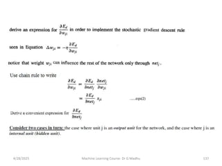
    DERIVATION OF THEGRADIENT DESCENT RULE 4/28/2025 Machine Learning Course- Dr G Madhu 111
  • 112.
    • Since thegradient specifies the direction of steepest increase of E, the training rule for gradient descent is 4/28/2025 Machine Learning Course- Dr G Madhu 112
  • 113.
    4/28/2025 Machine LearningCourse- Dr G Madhu 113 Source: Machine Learning, Tom Mitchell, McGraw Hill, 1997.
  • 114.
    4/28/2025 Machine LearningCourse- Dr G Madhu 114
  • 115.
    Feature of GradientDescent Algorithm 4/28/2025 Machine Learning Course- Dr G Madhu 115
  • 116.
    Stochastic Approximation toGradient Descent 4/28/2025 Machine Learning Course- Dr G Madhu 116
  • 117.
    4/28/2025 Machine LearningCourse- Dr G Madhu 117
  • 118.
    Differences Between StandardGradient Descent and Stochastic Gradient Descent 4/28/2025 Machine Learning Course- Dr G Madhu 118
  • 119.
    Remarks • We haveconsidered two similar algorithms for iteratively learning perceptron weights. • The key difference between these algorithms is that the perceptron training rule updates weights based on the error in the thresholded perceptron output, whereas the delta rule updates weights based on the error in the un-thresholded linear combination of inputs. 4/28/2025 Machine Learning Course- Dr G Madhu 119
  • 120.
    • The differencebetween these two training rules is reflected in different convergence properties. – The perceptron training rule converges after a finite number of iterations to a hypothesis that perfectly classifies the training data, provided the training examples are linearly separable. – The delta rule converges only asymptotically toward the minimum error hypothesis, possibly requiring unbounded time, but converges regardless of whether the training data are linearly separable. 4/28/2025 Machine Learning Course- Dr G Madhu 120
  • 121.
    Multilayer Networks andthe Backpropagation Algorithm • Single perceptrons can only express linear decision surfaces. • In contrast, the kind of multilayer networks learned by the BACKPROPACATION algorithm are capable of expressing a rich variety of nonlinear decision surface. • This section discusses how to learn such multilayer networks using a gradient descent algorithm. 4/28/2025 Machine Learning Course- Dr G Madhu 121
  • 122.
    4/28/2025 Machine LearningCourse- Dr G Madhu 122 • The network shown here was trained to recognize 1 of 10 vowel sounds occurring in the context "h_d" (e.g., "had," "hid"). • The network input consists of two parameters, F1 and F2, obtained from a spectral analysis of the sound. • The 10 network outputs correspond to the 10 possible vowel sounds. • The network prediction is the output whose value is highest. The plot on the right illustrates the highly nonlinear decision surface represented by the learned network. • Points shown on the plot are test examples distinct from the examples used to train the network. Source: Machine Learning, Tom Mitchell, McGraw Hill, 1997.
  • 123.
    A Differentiable ThresholdUnit • What type of unit shall we use as the basis for constructing multilayer networks? • At first we might be tempted to choose the linear units discussed in the previous section, for which we have already derived a gradient descent learning rule. • However, multiple layers of cascaded linear units still produce only linear functions, and we prefer networks capable of representing highly nonlinear functions. 4/28/2025 Machine Learning Course- Dr G Madhu 123
  • 124.
    • The perceptronunit is another possible choice, but its discontinuous threshold makes it undifferentiable and hence unsuitable for gradient descent. • What we need is a unit whose output is a nonlinear function of its inputs, but whose output is also a differentiable function of its inputs. • One solution is the sigmoid unit: – a unit very much like a perceptron, but based on a smoothed, differentiable threshold function. 4/28/2025 Machine Learning Course- Dr G Madhu 124
  • 125.
    The Sigmoid ThresholdUnit • The sigmoid unit is illustrated in following Figure. • Like the perceptron, the sigmoid unit first computes a linear combination of its inputs, then applies a threshold to the result. • In the case of the sigmoid unit, however, the threshold output is a 4/28/2025 Machine Learning Course- Dr G Madhu 125
  • 126.
    4/28/2025 Machine LearningCourse- Dr G Madhu 126
  • 127.
    The BACKPROPAGATION Algorithm •The BACKPROPAGATION Algorithm learns the weights for a multilayer network, given a network with a fixed set of units and interconnections. • It employs gradient descent to attempt to minimize the squared error between the network output values and the target values for these outputs. 4/28/2025 Machine Learning Course- Dr G Madhu 127
  • 128.
    Forward and Backwardpasses in Neural Networks • To train a neural network, there are 2 passes (phases): – Forward – Backward • In the forward pass, we start by propagating the data inputs to the input layer, go through the hidden layer(s), measure the network’s predictions from the output layer, and finally calculate the network error based on the predictions the network made. 4/28/2025 Machine Learning Course- Dr G Madhu 128
  • 129.
    4/28/2025 Machine LearningCourse- Dr G Madhu 129
  • 130.
    4/28/2025 Machine LearningCourse- Dr G Madhu 130 • This network error measures how far the network is from making the correct prediction. The forward and backward phases are repeated from some epochs. In each epoch, the following occurs: 1.The inputs are propagated from the input to the output layer. 2.The network error is calculated. 3.The error is propagated from the output layer to the input layer.
  • 131.
    • In thebackward pass, the flow is reversed so that we start by propagating the error to the output layer until reaching the input layer passing through the hidden layer(s). • The process of propagating the network error from the output layer to the input layer is called backward propagation, or simple backpropagation. • The backpropagation algorithm is the set of steps used to update network weights to reduce the network error. 4/28/2025 Machine Learning Course- Dr G Madhu 131
  • 132.
    • In BACKPROPAGATIONalgorithm, we consider networks with multiple output units rather than single units as before, so we redefine E to sum the errors over all of the network output units. 4/28/2025 Machine Learning Course- Dr G Madhu 132
  • 133.
  • 134.
    4/28/2025 Machine LearningCourse- Dr G Madhu 134
  • 135.
    4/28/2025 Machine LearningCourse- Dr G Madhu 135
  • 136.
    4/28/2025 Machine LearningCourse- Dr G Madhu 136
  • 137.
    4/28/2025 Machine LearningCourse- Dr G Madhu 137
  • 138.
    4/28/2025 Machine LearningCourse- Dr G Madhu 138
  • 139.
    4/28/2025 Machine LearningCourse- Dr G Madhu 139
  • 140.
    4/28/2025 Machine LearningCourse- Dr G Madhu 140
  • 141.
    4/28/2025 Machine LearningCourse- Dr G Madhu 141
  • 142.
    1.Convergence and LocalMinima • Backpropagation is only guaranteed to converge to a local, and not a global, minima. • However, since each weight in a network essentially corresponds to a different dimension in the error space, a local minimum with respect to one weight may not be a local minimum with respect to other weights. • This can provide an “escape route” from becoming trapped in local minima. 4/28/2025 Machine Learning Course- Dr G Madhu 142
  • 143.
    • If theweights are initialized to values close to zero, the sigmoid threshold function is approximately linear and so they produce linear outputs. • As the weights grow, though, the network is able to represent more complex functions that are not linear in nature. • It is the hope that by the time the weights are able to approximate the desired function that they will be close enough to the global minimum that even becoming stuck in a local minima will be acceptable. 4/28/2025 Machine Learning Course- Dr G Madhu 143
  • 144.
    Common Heuristic methodsto reduce the problem of local minima are: • Add a momentum term to the weight-update rule. • Use stochastic gradient descent rather than true gradient descent. • Train multiple networks using the same training data but initialize the networks with different random weights. • If the different networks lead to different local minima, choose the network that performs best on a validation set of data or all networks can be kept and treated as a committee whose output is the (possibly weighted) average of individual network outputs. 4/28/2025 Machine Learning Course- Dr G Madhu 144
  • 145.
    • A localminimum of a function is a point where the function value is smaller than at nearby points, but possibly greater than at a distant point. • A global minimum is a point where the function value is smaller than at all other feasible points. 4/28/2025 Machine Learning Course- Dr G Madhu 145
  • 146.
    4/28/2025 Machine LearningCourse- Dr G Madhu 146
  • 147.
    4/28/2025 Machine LearningCourse- Dr G Madhu 147
  • 148.
    4/28/2025 Machine LearningCourse- Dr G Madhu 148
  • 149.
    4/28/2025 Machine LearningCourse- Dr G Madhu 149
  • 150.
    4/28/2025 Machine LearningCourse- Dr G Madhu 150
  • 151.
    4/28/2025 Machine LearningCourse- Dr G Madhu 151
  • 152.
    Recurrent Neural Network •A recurrent neural network (RNN) is a class of artificial neural networks where connections between nodes form a directed or undirected graph along a temporal sequence. • This allows it to exhibit temporal dynamic behaviour. • Derived from feedforward neural networks, RNNs can use their internal state (memory) to process variable length sequences of inputs 4/28/2025 Machine Learning Course- Dr G Madhu 152
  • 153.
    4/28/2025 Machine LearningCourse- Dr G Madhu 153
  • 154.
    • Recurrent neuralnetworks (RNN) are the state of the art algorithm for sequential data and are used by Apple's Siri and and Google's voice search. • It is the first algorithm that remembers its input, due to an internal memory, which makes it perfectly suited for machine learning problems that involve sequential data. 4/28/2025 Machine Learning Course- Dr G Madhu 154
  • 155.
    4/28/2025 Machine LearningCourse- Dr G Madhu 155
  • 156.
    4/28/2025 Machine LearningCourse- Dr G Madhu 156 Recurrent Neural Network (RNN) Feed-forward Neural Network – Multilayer Perceptron (MLP)