Noname manuscript No.(will be inserted by the editor)A c.docx

Noname manuscript No.
(will be inserted by the editor)
A combined first and second order variational approach
for image reconstruction
Konstantinos Papafitsoros · Carola-Bibiane Schönlieb
July 10, 2012
Abstract In this paper we study a variational prob-
lem in the space of functions of bounded Hessian. Our
model constitutes a straightforward higher-order ex-
tension of the well known ROF functional (total vari-
ation minimisation) to which we add a non-smooth
second-order regulariser. It combines convex functions
of the total variation and the total variation of the
first derivatives. In what follows, we prove existence
and uniqueness of minimisers of the combined model
and present the numerical solution of the correspond-
ing discretised problem by employing the split Breg-

man method. The paper is furnished with applications
of our model to image denoising, deblurring as well
as image inpainting. The obtained numerical results
are compared with results obtained from TGV (total
generalised variation), infimal convolution and Euler’s
elastica, three other state of the art higher-order mod-
els. The numerical discussion confirms that the pro-
posed higher-order model competes with models of its
kind in avoiding the creation of undesirable artifacts
and blocky-like structures in the reconstructed images
– a known disadvantage of the ROF model – while be-
ing simple and efficiently numerically solvable.
Keywords Functions of bounded Hessian · Split
Bregman · Denoising · Deblurring · Inpainting ·
Staircasing
Mathematics Subject Classification (2000)
49J52 · 65K10 · 65N21 · 90C25 · 52A41 · 68U10
K. Papafitsoros
Cambridge Centre for Analysis, Department of Applied
Mathematics and Theoretical Physics, University of Cam-
bridge, Wilberforce Road, Cambridge CB3 0WA,

E-mail: [email protected]
C.B.Schönlieb
Cambridge Centre for Analysis, Department of Applied
Mathematics and Theoretical Physics, University of Cam-
bridge, Wilberforce Road, Cambridge CB3 0WA,
E-mail: [email protected]
1 Introduction
We consider the following general framework of a com-
bined first and second order non-smooth regularisa-
tion procedure. For a given datum u0 ∈ Ls(Ω), Ω ⊂
R2, s = 1, 2, we compute a regularised reconstruction
u as a minimiser of a combined first and second order
functional H(u). More precisely, we are interested in
solving
min
u
{
H(u) =
1
s
ˆ
Ω
|u0 −Tu|s dx + α
ˆ
Ω

f(∇ u) dx
+β
ˆ
Ω
g(∇ 2u) dx
}
, (1.1)
for s ∈ {1, 2}, non-negative regularisation parameters
α,β, convex functions f : R2 → R+, g : R4 → R+
with at most linear growth at infinity, and a suitable
linear operator T , see Section 3 for details. The ap-
propriate space for this minimisation is the space of
functions of bounded Hessian BH(Ω) which consists
of all functions u ∈ W1,1(Ω) such that ∇ u is a function
of bounded variation. The idea of this combination of
first and second order dynamics is to regularise with
a fairly large weight α in the first order term – pre-
serving the jumps as good as possible – and using a
small weight β for the second order term such that
artifacts (staircasing) created by the first order regu-
lariser are eliminated without introducing any serious

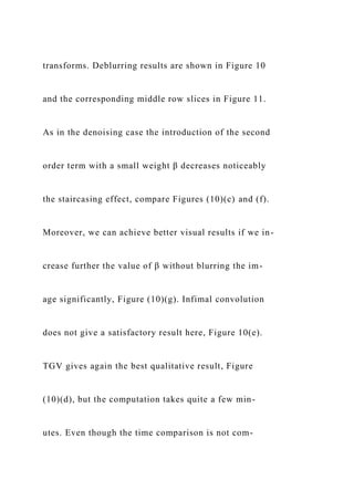
blur in the reconstructed image. We will show that for
image denoising, deblurring as well as inpainting the
model (1.1) offers solutions whose quality (accessed
by an image quality measure) is not far off from the
ones produced by some of the currently best higher-
order reconstruction methods in the field, e.g., the
recently proposed total generalised variation (TGV)
model [14]. Moreover, the computational effort needed
for its numerical solution is not much more than the
one needed for solving the standard ROF model [60].
For comparison the numerical solution for TGV reg-
ularisation is in general about ten times slower than
this, see Table 1 at the end of the paper.
In this paper we prove existence and uniqueness
of (1.1) for the classical setting of the problem in the
space W2,1(Ω) by means of relaxation. The general-
ity of this result includes both the classical variational

formulation in W2,1, e.g. for the Huber regularised ver-
sion of the total variation, as well as the non-smooth
norm minimisation setting in BH(Ω), which consti-
tutes the relaxed version of (1.1). In the numerical
part of the paper a discretised version of (1.1) is min-
imised by means of an operator splitting technique for
the cases f(x) = |x| and g(x) = |x|, and its appli-
cation to image denoising, deblurring and inpainting
is discussed. The rest of this section is structured as
follows. In Section 1.1 we phrase the general inverse
problem for image reconstruction, which leads us to
non-smooth norm minimisation, e.g. total variation
minimisation, and eventually to the introduction of
higher-order regularisers within this class. This sec-
tion is followed by a presentation of state of the art
higher-order methods in imaging in Section 1.2 and a
discussion of some models from this group which are
closely related to (1.1) in Section 1.3.

1.1 Context
A general inverse problem in imaging reads as follows.
Observing or measuring data u0 ∈ H in a suitable
Hilbert space of real functions defined on a domain
Ω, we seek for the original or reconstructed image u
that fulfils the model
u0 = Tu + n, (1.2)
where T is a linear operator in H, i.e., T ∈ L(H), and
n = n(u0) denotes a possible noise component which
– depending on the noise statistics – might depend on
the data u0. The operator T is the forward operator
of this problem. Examples are blurring operators (in
which case Tu denotes the convolution of u with a
blurring kernel), T = F the Fourier transform or T =
Pn a projection operator onto a subspace of H (i.e.,
only a few samples of u are given).
To reconstruct u one has to invert the operator T .
This is not always possible since in many applications
a problem can be ill-posed and further complicated by
interferences like noise. In this case a common proce-

dure in inverse problems is to add a-priori information
to the model, which in general is given by a certain
regularity assumption on the image u. Hence, instead
of solving (1.2) one computes u as a minimiser of
J(u) = Φ (u0,Tu) + αψ(u),
defined in a suitable Banach space Hψ. Here, ψ models
the regularity assumption on u with a certain regular-
ity parameter α > 0 and is called the regulariser of the
problem, and Φ is a distance function in H that en-
forces (1.2). The latter depends on the statistics of the
data u0, which can be either estimated or are known
from the physics behind the acquisition of u0. For u0
corrupted by normally distributed additive noise, this
distance function is the squared L2 norm of u0 −Tu.
For the choice of the regulariser ψ, squared Hilbert
space norms have a long tradition in inverse problems.
The most prominent example is H1 regularisation
min
u∈ H1
{
1

2
‖u0 −Tu‖2L2(Ω) + α‖∇ u‖
2
L2(Ω)
}
, (1.3)
see also [74, 67]. For T = Id, the gradient flow of
the corresponding Euler-Lagrange equation of (1.3)
reads ut = α∆u − u + u0. The result of such a reg-
ularisation technique is a linearly, i.e., isotropically,
smoothed image u, for which the smoothing strength
does not depend on u0. Hence, while eliminating the
disruptive noise in the given data u0 also prominent
structures like edges in the reconstructed image are
blurred. This observation gave way to a new class of
non-smooth norm regularisers, which aim to eliminate
noise and smooth the image in homogeneous areas,
while preserving the relevant structures such as ob-
ject boundaries and edges. More precisely, instead of
(1.3) one considers the following functional over the

space W1,1(Ω):
J(u) =
1
2
‖u0 −Tu‖2L2(Ω) +
ˆ
Ω
f(∇ u) dx, (1.4)
where f is a function from R2 to R+ with at most
linear growth, see [69]. As stated in (1.4) the min-
imisation of J over W1,1(Ω) is not well-posed in gen-
eral. For this reason relaxation procedures are applied,
which embed the optimisation for J into the opti-
misation for its lower semicontinuous envelope within
the larger space of functions of bounded variation, see
Section 2. The most famous example in image pro-
cessing is f(x) = |x|, which for T = Id results in
the so-called ROF model [60]. In this case the relaxed
formulation of (1.4) is the total variation denoising
model, where ‖∇ u‖L1(Ω) is replaced by the total vari-
ation |Du|(Ω) and J is minimised over the space of
functions of bounded variation. Other examples for
f are regularised versions of the total variation like

f(x) =
√
x2 + �2 for a positive � � 1 [1, 40], the
Huber-regulariser and alike [27, 46, 21, 53]. The con-
sideration of such regularised versions of |∇ u| is some-
times of advantage in applications where perfect edges
are traded against a certain smoothness in homoge-
neous parts of the image, [57]. Moreover such regular-
isations become necessary for the numerical solution
of (1.4) by means of time-stepping [69] or multigrid-
methods [70, 42, 68] for instance.
As these and many more contributions in the im-
age processing community have proven, this new non-
smooth regularisation procedure indeed results in a
nonlinear smoothing of the image, smoothing more in
homogeneous areas of the image domain and preserv-
ing characteristic structures such as edges. In partic-
ular, the total variation regulariser is tuned towards
2

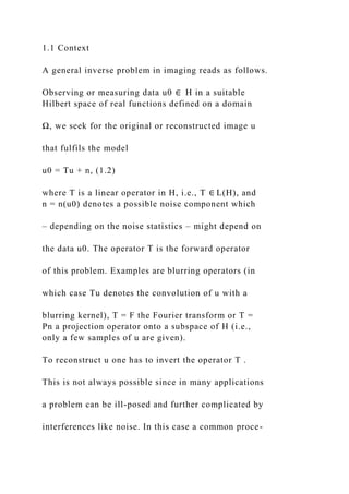
the preservation of edges and performs very well if
the reconstructed image is piecewise constant. The
drawback of such a regularisation procedure becomes
apparent as soon as one considers images or signals
(in 1D) which do not only consist of flat regions and
jumps, but also possess slanted regions, i.e. piecewise
linear parts. The artifact introduced by total varia-
tion regularisation in this case is called staircasing.
Roughly this means that the total variation regulari-
sation of a noisy linear function u0 in one dimension
is a staircase u, whose L2 norm is close to u0, see Fig-
ure 1. In one dimension this effect has been rigorously
studied in [30]. In two dimensions this effect results in
blocky-like images, see Figure 2.
One way to reduce this staircasing effect is in fact
to “round off” the total variation term by using reg-
ularised versions defined by functions f as indicated

above, e.g., Huber regularisation [57]. However, such
a procedure can only reduce these artifacts to a cer-
tain extent. For instance, the Huber-type regularisa-
tion will eliminate the staircasing effect only in areas
with small gradient. Another way of improving total
variation minimisation is the introduction of higher-
order derivatives in the regulariser as in (1.1). Espe-
cially in recent years, higher-order versions of non-
smooth image enhancing methods have been consid-
ered.
1.2 Related work
Already in the pioneering paper of Chambolle and Li-
ons [21] the authors propose a higher-order method
by means of an inf-convolution of two convex regu-
larisers. Here, a noisy image is decomposed into three
parts u0 = u1 + u2 + n by solving
min
(u1,u2)
{ 1

2
‖u0 −u1 −u2‖2L2(Ω) + α
ˆ
Ω
|∇ u1| dx
+β
ˆ
Ω
|∇ 2u2| dx
}
, (1.5)
where ∇ 2u2 is the distributional Hessian of u2. Then,
u1 is the piecewise constant part of u0, u2 the piece-
wise smooth part and n the noise (or texture). Along
these lines a modified infimal-convolution approach
has been recently proposed in the discrete setting in
[64, 65]. Another attempt to combine first and second
order regularisation originates from Chan, Marquina,
and Mulet [25], who consider total variation minimisa-
tion together with weighted versions of the Laplacian.
More precisely, they consider a regularising term of

the form
α
ˆ
Ω
|∇ u| dx + β
ˆ
Ω
f(|∇ u|)(∆u)2 dx,
where f must be a function with certain growth con-
ditions at infinity in order to allow jumps. The well-
posedness of the latter in one space dimension has
been rigorously analysed by Dal Maso, Fonseca, Leoni
and Morini [30] via the method of relaxation.
The idea of bounded Hessian regularisers was also
considered by Lysaker et al. [51, 52], Chan et al. [26],
Scherzer et al. [61, 47], Lai at al. [49] and Bergounioux
and Piffet [8]. In these works the considered model has
the general form
min
u

{
1
2
‖u0 −u‖2L2(Ω) + α|∇
2u|(Ω)
}
.
In Lefkimmiatis et al. [50], the spectral norm of the
Hessian matrix is considered. Further, in [59] minimis-
ers of functionals which are regularised by the total
variation of the (l− 1)st derivative, i.e.,
|D∇ l−1u|(Ω),
are studied. Another interesting higher-order total vari-
ation model is proposed by Bredies et al. [14]. The con-
sidered regulariser is called total generalised variation
(TGV) and is of the form
TGV kα (u) = sup
{ˆ
Ω
udivkξ dx :
ξ ∈ Ckc (Ω, Sym

k(Rd)),
‖divlξ‖∞ ≤ αl, l = 0, . . . ,k − 1
}
, (1.6)
where Symk(Rd) denotes the space of symmetric ten-
sors of order k with arguments in Rd, and αl are fixed
positive parameters. Its formulation for the solution
of general inverse problems was given in [15].
Properties of higher-order regularisers in the dis-
crete setting in terms of diffusion filters are further
studied in [33]. Therein, the authors consider the Euler-
Lagrange equations corresponding to minimisers of
functionals of the general type
J(u) =
ˆ
Ω
(u0 −u)2 dx + α
ˆ
Ω
f
|β|=p

|Dβu|2
(1.7)
for different non-quadratic penaliser functions f. More-
over, Bertozzi and Greer [10] have rigorously studied
the fourth-order evolution equation which arises as a
gradient flow of
´
G(∆u), where G is a nondecreasing
function of quadratic growth in a neighbourhood of 0
and at most linear growth at infinity.
Solution
s of this
model are called low curvature image simplifiers and
are given by
ut = −α∆(arctan(∆u)) + (u0 −u),

when G(s) = s arctan(s) − 1/2 log(s2 + 1).
Higher-order inpainting methods in general per-
form much better than first order methods – like total
variation inpainting – because of the additional direc-
tional information used for the interpolation process.
Euler’s elastica is a popular higher-order variational
method [24, 66]. There, the regularising term reads:
ˆ
Ω
(
α + β
(
∇ ·
∇ u
|∇ u|
)2)

|∇ u| dx,
3
(a) Noisy, piecewise linear signal (b) First order total variation
denoised signal
Fig. 1 Illustration of the staircasing effect in one space
dimension
�
��
Fig. 2 First order image denoising and the staircasing effect: (l.)
noisy image, (m.) denoised image, (r.) detail of the bottom
right hand corner of the denoised image to visualise the
staircasing effect (the creation of blocky-like patterns due to the
first order regulariser)
i.e., is a combination of the total variation and the
curvature of the level lines of u (a nonlinear second

order regularising term). Other examples of higher-
order inpainting are the Cahn-Hilliard inpainting [9],
TV-H−1 inpainting [16, 62] and Hessian-based surface
restoration [49].
1.3 Relation of our model to TGV, infimal
convolution regularisation, higher-order diffusion
filters and Euler’s elastica
In this section we want to analyse the connection of
our combined 1st and 2nd order approach (1.1) with
infimal convolution (1.5) [21, 64, 65], the generalised
total variation regulariser (1.6) of order two [14] and
with higher-order diffusion filters [33]. Moreover, in
the case of inpainting, we discuss the connection of

our model to Euler’s elastica [24, 66].
In the case of inf-convolution (1.5) the regularised
image u = u1 + u2 consists of a function u1 ∈ BV (Ω)
and a function u2 ∈ BH(Ω) which are balanced against
each other by positive parameters α,β. Differently,
a minimiser u of (1.1) is in BH(Ω) as a whole and
as such is more regular than the infimal convolution
minimiser which is a function in BV (Ω). Hence, infi-
mal convolution reproduces edges in an image as per-
fect jumps while in our combined first and second
order total variation approach edges are lines where
the image function has a large but finite gradient ev-
erywhere. We believe that our approach (1.1) can be
made equivalent to infimal convolution if combined

with the correct choice of adaptive regularisation, e.g.,
[34, 41]. More precisely, we replace the two constant
parameters α and β by spatially varying functions
α(x),β(x) and minimise for u
1
2
ˆ
Ω
(u0 −u)2 dx +
ˆ
Ω
α|∇ u| dx +
ˆ
Ω
β|∇ 2u| dx.

Then, we can choose α and β according to (1.5), i.e.,
α = 0 where u = u2, β = 0 where u = u1, and α/β
correctly balancing u1 and u2 in the rest of Ω. How-
ever, let us emphasise once more that this is not our
intention here.
The relation of (1.1) to the regularisation approach
with total generalised variation [14] of order 2 can be
understood through its equivalence with the modified
infimal convolution approach [65] in the discrete set-
ting. The total generalised variation of order 2 is de-
fined for a positive multi-index α = (α0,α1) as
TGV 2α (u) = sup
{ˆ

Ω
u div2v dx :
v ∈ C2c (Ω, Sym
2(Rd)),
‖divlv‖∞ ≤ αl, l = 0, 1
}
,
where Sym2(Rd) is the space of symmetric tensors of
order 2 with arguments in Rd. For smooth enough
4
functions u the second order TGV can be written as
TGV 2α (u) = inf
u1+u2=u
w1∈ ker�1, w2∈ ker�2

{
α0
ˆ
Ω
|∇ 2u1 + w1| dx
+α1
ˆ
Ω
|∇ u2 + w2| dx
}
,
for a positive multiindex (α,β) and �l = 1
2
(∇ ul +
∇ u⊥ l ). In this case TGV
2
α is equivalent to the mod-

ified infimal convolution regulariser proposed in [65].
The relation to higher-order diffusion filters as anal-
ysed in [33] becomes apparent when considering the
Euler-Lagrange equation of (1.1) in the case T = Id
and f, g having the form f(x) = h(|x|), g(x) = h(|x|),
where h is convex and has at most linear growth.
Namely, with appropriate boundary conditions we ob-
tain the following Euler-Lagrange equation
u−u0 = α div
(
h′(|∇ u|)
∇ u
|∇ u|
)
(1.8)

−βdiv2
(
h′(|∇ 2u|)
∇ 2u
|∇ 2u|
)
.
This simplifies for the case h(x) =
√
|x|2 + �2 to a
regularised total variation/bounded Hessian reaction-
diffusion equation that reads
u−u0 = α div
(
∇ u√
|∇ u|2 + �2

)
−βdiv2
(
∇ 2u√
|∇ 2u|2 + �2
)
.
The consideration of corresponding evolution equa-
tions for (1.8) in the presence of different choices of
penalising functions h promises to give rise to addi-
tional properties of this regularisation technique and
is a matter of future research.
As far as inpainting is concerned, we examine here
the connection of our method to Euler’s elastica. De-

pending on how each of the terms in the Euler’s elas-
tica regulariser are weighted, the interpolation process
is performed differently. If a larger weight is put on the
total variation the interpolation results into an image
with sharp edges, which however can get disconnected
if the scale of the gap is larger than the scale of the
object whose edges should be propagated into it. This
behaviour is a validation of the so-called “good contin-
uation principle” defined by the Gestaltist school [48]
and not desirable in image inpainting. Putting a larger
weight on the curvature term however resolves this is-
sue and gives satisfying results with respect to the con-

tinuation principle. The right combination (balance)
of these two terms seems to result into a good trade-
off between “sharpness” and “continuation” of edges.
However, one disadvantage of the Euler’s elastica in-
painting model for analytic and numerical issues is
that it is a non-convex minimisation problem. In par-
ticular, numerical algorithms are in general not guar-
anteed to converge to a global minimiser, only local
minimisation can be achieved. The minimisation of
functional (1.1) can be seen as a convex simplification
of the Euler’s elastica idea, where we have replaced the
non-convex curvature by the convex total variation of
the first derivative of u.

For more discussion and comparison of higher-order
regularisers we recommend Chapters 4.1.5-4.1.7 and
6.4 in [5].
Outline of the paper: In Section 2 we give a brief intro-
duction to Radon measures, convex functions of mea-
sures and functions of bounded variation. In Section
3 we introduce the variational problem (1.1) and the
space BH(Ω) that this functional is naturally defined
in. We define two topologies on BH(Ω) and we iden-
tify the lower semicontinuous envelope of (1.1) with
respect to these topologies. Finally, we prove the well-
posedness – existence, uniqueness, stability – of the

minimisation of the relaxed functional using standard
techniques from calculus of variations. Section 4 deals
with two special versions of (1.1), the anisotropic ver-
sion and the case with the L1 norm in the fidelity
term. In Section 5 we introduce the corresponding
discretised problem and we propose the split Breg-
man method for its numerical implementation in the
case f(x) = |x|, g(x) = |x|. In Sections 6, 7 and 8
we present some numerical examples of our method
in image denoising, deblurring and inpainting respec-
tively. Finally, in Section 9 we discuss how our ap-
proach compares with other higher-order methods like
infimal convolution (denoising, deblurring), total gen-

eralised variation (denoising, deblurring) and Euler’s
elastica (inpainting).
2 Preliminaries
In this section, we introduce some basic notions that
we are going to use. A reader familiar with Radon
measures, BV functions and relaxed functionals can
quickly go through Sections 2.1, 2.3 and 2.4 respec-
tively. Section 2.2 familiarises the reader with convex
functions of measures, a perhaps less known subject.
Remarks on standard notation: As usual, we de-
note with Ln the Lebesgue measure. Different notions
are denoted by | · |: When it is applied on vectors or
matrices it denotes the Euclidean norm (vector) or
the Frobenius norm (matrices). When it is applied on

measures it denotes the total variation measure while
when it is applied on Borel subsets of Rn it denotes
the Lebesgue measure of that subset. Finally, | · |1 de-
notes the `1 norm in Rn and (·, ·) denotes the standard
Euclidean inner product.
5
2.1 Finite Radon measures
All our notation and definitions are consistent with [4].
From now on, Ω denotes an open set in Rn. We define
the space [M(Ω)]m to be the space of Rm-valued finite
Radon measures. The total variation measure of µ ∈
[M(Ω)]m is denoted by |µ|. We say that a sequence
(µk)k∈ N in [M(Ω)]m converges weakly∗ to a measure
µ ∈ [M(Ω)]m if limk→∞
´
Ω

udµk =
´
Ω
udµ for all
u ∈ C0(Ω), the completion of Cc(Ω) endowed with
the supremum norm. Thus (µk)k∈ N converges weakly
∗
to µ if it converges weakly∗ component-wise. We will
often consider the Lebesgue decomposition of a Rm-
valued finite Radon measure µ with respect to a σ-
finite positive Borel measure ν :
µ = µa + µs =
(µ
ν
)
ν + µs,

where µa is the absolutely continuous part of µ with
respect to ν, µs is the singular part and (µ/ν) denotes
the density function of µ with respect to ν (Radon-
Nikodým derivative). Again this is nothing else than
the usual Lebesgue decomposition regarded component-
wise. Recall also that any µ ∈ [M(Ω)]m is absolutely
continuous with respect to |µ| and thus we obtain the
polar decomposition of µ
µ =
(
µ
|µ|
)
|µ|, with
∣ ∣ ∣ ∣ µ|µ|

∣ ∣ ∣ ∣ = 1, |µ| a.e..
2.2 Convex functions of measures
Let g be a continuous function from Rm to R which
is positively homogeneous of degree 1, i.e., for every
x ∈ Rm
g(tx) = tg(x), ∀ t ≥ 0.
Given a measure µ ∈ [M(Ω)]m, we define the R-
valued measure g(µ) as follows:
g(µ) := g
(
µ
|µ|
)
|µ|.
It can be proved that if g is a convex function then

g(·) is a convex function in [M(Ω)]m and if ν is any
positive measure such that µ is absolutely continuous
with respect to ν then
g(µ) = g
(µ
ν
)
ν.
We refer the reader to Proposition A.1 in Appendix A
for a proof of the above statement. Suppose now that
g is not necessarily positively homogeneous but it is
a continuous function from Rm → R which is convex
and has at most linear growth at infinity, i.e., there
exists a positive constant K such that
|g(x)| ≤ K(1 + |x|), ∀ x ∈ Rm.

In that case the recession function g∞ of g is well
defined everywhere, where
g∞(x) := lim
t→∞
g(tx)
t
, ∀ x ∈ Rm.
It can be proved that g∞ is a convex function and
positively homogeneous of degree 1. Given a measure
µ ∈ [M(Ω)]m we consider the Lebesgue decomposi-
tion with respect to the Lebesgue measure Ln, µ =
(µ/Ln)Ln + µs and we define the R-valued measure
g(µ) as follows:
g(µ) = g
( µ
Ln

)
Ln + g∞(µs)
= g
( µ
Ln
)
Ln + g∞
(
µs
|µs|
)
|µs|. (2.1)
We refer the reader to Theorem A.2 in Appendix A
for a result regarding lower semicontinuity of convex
functions of measures with respect to the weak∗ con-
vergence.

2.3 The space [BV (Ω)]m
We recall that a function u ∈ L1(Ω) is said to be a
function of bounded variation or else u ∈ BV (Ω) if
its distributional derivative can be represented by a
Rn-valued finite Radon measure. This means thatˆ
Ω
u∂iφ dx = −
ˆ
Ω
φ dDiu, ∀ φ ∈ C1c (Ω), i = 1, . . . ,n.
for some Rn-valued finite Radon measure Du =
(D1u,. . . ,Dnu). It is immediate that W
1,1(Ω)⊆BV (Ω)
since if u ∈ W1,1(Ω) then Du = ∇ uLn. Consistently,
we say that a function u = (u1, . . . ,um) ∈ [L1(Ω)]m
belongs to [BV (Ω)]m if
ˆ
Ω

ua∂iφ dx = −
ˆ
Ω
φ dDiu
a, i = 1, . . . ,n,
a = 1, . . . ,m.
In that case Du is an m × n matrix-valued measure.
A function u belongs to [BV (Ω)]m if and only if its
variation in Ω, V (u,Ω) is finite, where,
V (u,Ω) = sup
{
m∑
a=1
ˆ
Ω
uadivφa dx :

φ ∈ [C1c (Ω)]
mn, ‖φ‖∞ ≤ 1
}
.
Moreover if u ∈ [BV (Ω)]m then |Du|(Ω) = V (u,Ω)
and if u ∈ [W1,1(Ω)]m, then |Du|(Ω) =
´
Ω
|∇ u|dx,
where |∇ u| =
(∑m
a=1
∑n
i=1(∂iu
a)2
)1/2
. The space

[BV (Ω)]m endowed with the norm ‖u‖BV (Ω) :=´
Ω
|u| dx+|Du|(Ω) is a Banach space. It can be shown
that if Du = 0, then u is equal to a constant a.e. in
any connected component of Ω.
Suppose that (uk)k∈ N, u belong to [BV (Ω)]
m. We
say that the sequence (uk)k∈ N converges to u weakly
∗
in [BV (Ω)]m if it converges to u in [L1(Ω)]m and the
6
sequence of measures (Duk)k∈ N converges weakly
∗ to
the measure Du. It is known that (uk)k∈ N converges

to u weakly∗ in [BV (Ω)]m if and only if (uk)k∈ N is
bounded in [BV (Ω)]m and converges to u in [L1(Ω)]m.
The usefulness of the introduction of the weak∗ con-
vergence is revealed in the following compactness re-
sult: Suppose that the sequence (uk)k∈ N is bounded
in [BV (Ω)]m, where Ω is a bounded open set of Rn
with Lipschitz boundary. Then there exists a subse-
quence (uk`)`∈ N and a function u ∈ [BV (Ω)]
m such
that (uk`)`∈ N converges to u weakly
∗ in [BV (Ω)]m.
We say that the sequence (uk)k∈ N converges to u
strictly in [BV (Ω)]m if it converges to u in [L1(Ω)]m
and (|Duk|(Ω))k∈ N converges to |Du|(Ω). It is imme-

diate that strict convergence implies weak∗ conver-
gence.
Suppose that Ω is bounded with Lipschitz bound-
ary. Define 1∗ = n/(n − 1) when n > 1 and 1∗ = ∞
when n = 1. Then BV (Ω) ⊆ L1
∗
(Ω) with continu-
ous embedding. Moreover if Ω is connected then the
following inequality holds (Poincaré-Wirtinger):
‖u−uΩ‖L1∗ (Ω) ≤ C|Du|(Ω), ∀ u ∈ BV (Ω),
where the constant C depends only on Ω and uΩ de-
notes the mean value of u in Ω:
uΩ :=
1

|Ω|
ˆ
Ω
u dx.
We refer the reader to [4] for a detailed description
of the above as well as for an introduction to weak
continuity and differentiability notions in BV (Ω) and
the decomposition of the distributional derivative of a
function u ∈ BV (Ω).
2.4 Relaxed functionals
Suppose that X is a set endowed with some topology
τ and let F : X → R∪ {+∞}. The relaxed functional
or otherwise called the lower semicontinuous envelope
of F with respect to the topology τ is a functional

F : X → R∪ {+∞} defined as follows for every x ∈ X:
F(x) = sup{G(x) : G : X → R∪ {+∞},
τ lower semicontinuous, G(y) ≤ F(y),
∀ y ∈ X}.
It is easy to check that F is the greatest τ lower semi-
continuous functional which is smaller or equal than
F. It can be also checked that
F(x) = sup
U∈ N(x)
inf
y∈ U
F(y),
where N(x) denotes the open neighbourhoods of x.
Moreover, if X is a first countable topological space,
then F(x) is characterised by the two following prop-

erties:
(i) For every sequence (xk)k∈ N converging to x, we
have
F(x) ≤ lim inf
k→∞
F(xk).
(ii) There exists a sequence (xk)k∈ N converging to x
such that
F(x) ≥ lim sup
k→∞
F(xk).
An interesting property of the relaxed functional is
that if it has a minimum point then the value of F at

that point will be equal with the infimum of F i.e.
min
x∈ X
F(x) = inf
x∈ X
F(x).
For more information on relaxed functionals see [29]
and [12].
3 The variational formulation
In the current section we specify our definition of the
functional (1.1) that we want to minimise. We start
by defining the minimisation problem in the space
W2,1(Ω) as this is the space in which our analysis
subsumes various choices for the regularisers f and

g. As this space is not reflexive, and thus existence
of minimisers cannot be guaranteed, we extend the
definition to a larger space. We introduce this larger
space BH(Ω) as the subspace of all u ∈ W1,1(Ω) such
that ∇ u ∈ [BV (Ω)]m. We define the weak∗ and the
strict topology of BH(Ω) and we identify the lower
semicontinuous envelope (relaxed functional) of the
extended functional with respect to these topologies.
We prove existence of minimisers of the relaxed func-
tional, uniqueness under some assumptions as well as
stability.
In the following Ω denotes as usual a bounded,
connected, open subset of R2 with Lipschitz bound-
ary, T denotes a bounded linear operator from L2(Ω)

to L2(Ω), u0 ∈ L2(Ω) and α, β are non-negative
constants. Further we suppose that f : R2 → R+,
g : R4 → R+ are convex functions with at most linear
growth at infinity, i.e., there exist positive constants
K1 and K2 such that
f(x) ≤ K1(1 + |x|), ∀ x ∈ R2, (3.1)
g(x) ≤ K2(1 + |x|), ∀ x ∈ R4. (3.2)
Moreover, we assume that both f and g are minimised
in 0 and they satisfy a coercivity condition:
f(x) ≥ K3|x|, ∀ x ∈ R2, (3.3)
g(x) ≥ K4|x|, ∀ x ∈ R4, (3.4)
where K3 and K4 are strictly positive. We want to
minimise the following functional:
H(u) =
1

2
ˆ
Ω
(u0 −T(u))2 dx + α
ˆ
Ω
f(∇ u) dx
+β
ˆ
Ω
g(∇ 2u) dx. (3.5)
7
The natural space for the functional H to be defined
in, is W2,1(Ω). Since this space is not reflexive a solu-

tion of the minimisation problem by the direct method
of calculus of variations does not work. Rather, exis-
tence of a minimiser of (3.5) can be shown via relax-
ation that is: We extend the functional H into a larger
space which has some useful compactness properties
with respect to some topology and we identify the re-
laxed functional with respect to the same topology.
This space is BH(Ω).
3.1 The space BH(Ω)
The space BH(Ω) (often denoted with BV 2(Ω)) is the
space of functions of bounded Hessian. It was intro-
duced by Demengel in [31] and consists of all functions

u ∈ W1,1(Ω) whose distributional Hessian can be rep-
resented by an R2 ×R2-valued finite Radon measure.
In other words:
BH(Ω) = {u ∈ W1,1(Ω) : ∇ u ∈ [BV (Ω)]2}.
We set D2u := D(∇ u). Again it is immediate that
W2,1(Ω) ⊆ BH(Ω). BH(Ω) is a Banach space equipped
with the norm ‖u‖BH(Ω) = ‖u‖BV (Ω) + |D2u|(Ω). If
Ω has a Lipschitz boundary and it is connected then
it can be shown that there exist positive constants C1
and C2 such that
ˆ
Ω
|∇ u|dx ≤ C1|D2u|(Ω)+C2
ˆ
Ω
|u|dx, ∀ u ∈ BH(Ω).
(3.6)

Moreover, the embedding from BH(Ω) into W1,1(Ω)
is compact, see [31]. We denote the approximate dif-
ferential of ∇ u with ∇ 2u, see [4] for a definition.
Analogously with BV (Ω) we define the following
notions of convergence in BH(Ω):
Definition 3.1 (Weak∗ convergence in BH(Ω)).
Let (uk)k∈ N, u belong to BH(Ω). We say that (uk)k∈ N
converges to u weakly∗ in BH(Ω) if
uk → u, in L1(Ω)
and
∇ uk ⇀ ∇ u weakly∗ in [BV (Ω)]2, as k →∞,
or in other words
‖uk −u‖L1(Ω) → 0,
‖∇ uk −∇ u‖[L1(Ω)]2 → 0,

ˆ
Ω
φ dD2uk →
ˆ
Ω
φ dD2u, ∀ φ ∈ C0(Ω).
It is not hard to check that a basis for that topology
consists of the following sets:
U(v,F,�) =
{
u ∈ BH(Ω) : ‖v −u‖L1(Ω)
+‖∇ v −∇ u‖[L1(Ω)]2
+
∣ ∣ ∣ ∣
ˆ
Ω

φi dD
2v −
ˆ
Ω
φi dD
2u
∣ ∣ ∣ ∣ < �,
i ∈ F
}
,
where v ∈ BH(Ω), F is finite, � > 0 and φi ∈ C0(Ω).
This topology is also metrizable, hence first countable.
We do not imply here that BH(Ω) is the dual space of
a Banach space but we name this convergence weak∗
to show the correspondence with the weak∗ conver-

gence in BV (Ω). We have also the corresponding com-
pactness result:
Theorem 3.2 (Compactness in BH(Ω)). Suppose
that the sequence (uk)k∈ N is bounded in BH(Ω). Then
there exists a subsequence (uk`)`∈ N and a function u ∈
BH(Ω) such that (uk`)`∈ N converges to u weakly
∗ in
BH(Ω).
Proof. From the compact embedding of BH(Ω) into
W1,1(Ω) and the fact that the sequence (∇ uk)k∈ N is
bounded in [BV (Ω)]2 we have that there exists a sub-
sequence (uk`)`∈ N, a function u ∈ W
1,1(Ω) and a func-
tion v ∈ [BV (Ω)]2 such that (uk`)`∈ N converges to
u in W1,1(Ω) and (∇ uk`)`∈ N converges to v weakly

∗
in [BV (Ω)]2, as ` goes to infinity. Then, ∇ u = v,
u ∈ BH(Ω) and (uk`)`∈ N converges to u weakly
∗ in
BH(Ω).
Definition 3.3 (Strict convergence in BH). Let
(uk)k∈ N, u belong to BH(Ω). We say that (uk)k∈ N
converges to u strictly in BH(Ω) if
uk → u, in L1(Ω)
and
|D2uk|(Ω) →|D2u|(Ω), as k →∞.
It is easily checked that the function
d(u,v) =

ˆ
Ω
|u−v| dx +
∣ ∣ |D2u|(Ω) −|D2v|(Ω)∣ ∣ ,
is a metric and induces the strict convergence in BH(Ω).
The following Lemma can be used to compare these
two topologies.
Lemma 3.4. Suppose that (uk)k∈ N, u belong to BH(Ω)
and (uk)k∈ N converges to u strictly in BH(Ω). Then
‖uk −u‖W1,1(Ω) → 0, as k →∞.
8
Proof. We recall from (3.6) that there exist positive
constants C1 and C2 such thatˆ

Ω
|∇ u|dx ≤ C1|D2u|(Ω)+C2
ˆ
Ω
|u|dx, ∀ u ∈ BH(Ω).
Since the sequence (uk)k∈ N is strictly convergent in
BH(Ω), the sequences (‖uk‖L1(Ω))k∈ N and
(|D2uk|(Ω))k∈ N are bounded. Hence, there exists a
positive constant C such that
ˆ
Ω
|∇ uk| dx < C, ∀ k ∈ N,
which implies that the sequence (uk)k∈ N is bounded
in BH(Ω). From the compact embedding of BH(Ω)
into W1,1(Ω) we get that there exists a subsequence
(uk`)`∈ N and a function v ∈ W

1,1(Ω) such that (uk`)`∈ N
converges to v in W1,1(Ω). In particular (uk`)`∈ N con-
verges to v in L1(Ω) so v = u and thus (uk`)`∈ N con-
verges to u in W1,1(Ω). Since every subsequence of
(uk)k∈ N is bounded in BH(Ω) we can repeat the same
argument and deduce that for every subsequence of
(uk)k∈ N there exists a further subsequence which con-
verges to u in W1,1(Ω). This proves that the initial
sequence (uk)k∈ N converges to u in W
1,1(Ω)
Corollary 3.5. Strict convergence implies weak∗ con-
vergence in BH(Ω).
3.2 Relaxation of the second order functional

We now extend the functional H in (3.5) to BH(Ω)
in the following way:
Hex(u) =
1
2
´
Ω
(u0 −Tu)2 dx
+α
´
Ω
f(∇ u) dx
+β
´
Ω

g(∇ 2u) dx if u ∈ W2,1(Ω),
+∞ if f ∈
BH(Ω) W2,1(Ω).
(3.7)
As we have discussed above, the weak∗ topology in
BH(Ω) provides a good compactness property which
is inherited from the weak∗ topology in [BV (Ω)]n.
However, the functional Hex is not sequentially lower
semicontinuous with respect to the strict topology in
BH(Ω) and hence it is neither with respect to the
weak∗ topology in BH(Ω). Indeed, we can find a func-
tion u ∈ BH(Ω)W2,1(Ω), see [31] for such an exam-
ple. Hence, from the definition of Hex we have Hex(u) =
∞. However, according to Theorem A.3 we can find a

sequence (uk)k∈ N in W
2,1(Ω) which converges strictly
to u. It follows that the sequences (‖uk‖L1(Ω))k∈ N,
(|D2uk|(Ω))k∈ N as well as (‖∇ uk‖L1(Ω))k∈ N are bounded.
Moreover the sequence (uk)k∈ N is bounded in L
2(Ω).
Since T is a bounded linear operator and from the fact
that f and g have at most linear growth at infinity we
deduce that the sequence (Hex(uk))k∈ N is bounded as
well. Hence we get
Hex(Ω) > lim inf
k→∞
Hex(uk),
which proves that Hex is not lower semicontinuous

with respect to the strict topology in BH(Ω). Thus,
we have to identify its lower semicontinuous envelope
with respect to the strict convergence. We define the
following functional in BH(Ω) :
Hex(u) :=
1
2
ˆ
Ω
(u0 −Tu)2dx + α
ˆ
Ω
f(∇ u) dx
+β g(D2u)(Ω)
=

1
2
ˆ
Ω
(u0 −Tu)2dx + α
ˆ
Ω
f(∇ u) dx
+β
ˆ
Ω
g(∇ 2u) dx
+β
ˆ
Ω

g∞
(
Ds∇ u
|Ds∇ u|
)
d|Ds∇ u|,
where ∇ 2u, the approximate differential of ∇ u, is also
the density of D2u with respect to the Lebesgue mea-
sure, see [4]. It is immediate to see that if u ∈ W2,1(Ω)
then Hex(u) = Hex(u). Thus is general, Hex is smaller
than Hex.
Theorem 3.6. The functional Hex is lower semicon-
tinuous with respect to the strict topology in BH(Ω).
Proof. It is not hard to check that since f is convex
and it has at most linear growth then it is Lipschitz,

say with constant L > 0. Let u and (uk)k∈ N be func-
tions in BH(Ω) and let (uk)k∈ N converge to u strictly
in BH(Ω) and thus also weakly∗ in BH(Ω). We have
to show that
Hex(u) ≤ lim inf
k→∞
Hex(un).
From the definition of the weak∗ convergence in BH(Ω)
we have that (uk)k∈ N converges to u in W
1,1(Ω). From
the Sobolev inequality, see [39],
‖v‖L2(Ω) ≤ C‖v‖W1,1(Ω), ∀ v ∈ W1,1(Ω),
we have that (uk)k∈ N converges to u in L
2(Ω). Since

T : L2(Ω) → L2(Ω) is continuous then the map u 7→
1
2
´
Ω
(u0 − Tu)2dx is continuous and hence we have
that
1
2
ˆ
Ω
(u0−Tuk)2dx →
1
2
ˆ
Ω

(u0−Tu)2dx, as k →∞.
(3.8)
Moreover since ‖∇ uk −∇ u‖[L1(Ω)]2 converges to 0 as
k →∞, we have from the Lipschitz property∣ ∣ ∣ ∣
ˆ
Ω
f(∇ uk) dx−
ˆ
Ω
f(∇ u) dx
∣ ∣ ∣ ∣ ≤
ˆ
Ω
|f(∇ uk) −f(∇ u)| dx ≤
9

L
ˆ
Ω
|∇ uk −∇ u| dx → 0, as k →∞,
i.e., we have
ˆ
Ω
f(∇ uk) dx →
ˆ
Ω
f(∇ u) dx, as k →∞. (3.9)
Finally we have that D2uk → D2u weakly∗ . We can
apply Theorem A.2 for µk = µ = L2, ν = D2u, νk =
D2uk and get that
g(D2u)(Ω) ≤ lim inf
k→∞
g(D2uk)(Ω). (3.10)

From (3.8), (3.9) and (3.10) we get that
Hex(u) ≤ lim inf
k→∞
Hex(uk).
Theorem 3.7. The functional Hex is the lower semi-
continuous envelope of Hex with respect to the strict
convergence in BH(Ω).
Proof. Suppose that (uk)k∈ N converges to u strictly in
BH(Ω). From the lower semicontinuity of Hex we have
that Hex(u) ≤ lim infk→∞Hex(uk) and since Hex ≤
Hex we get that Hex(u) ≤ lim infk→∞Hex(uk). For
the other direction Theorem A.3 tells us that given u ∈
BH(Ω) there exist a sequence (uk)k∈ N ⊆ C∞(Ω) ∩
W2,1(Ω) such that (uk)k∈ N converges to u strictly in
BH(Ω) and

g(D2uk)(Ω) → g(D2u)(Ω). (3.11)
We have also that (uk)k∈ N converges to u in W
1,1(Ω)
which implies that
1
2
ˆ
Ω
(u0 −Tuk)2dx + α
ˆ
Ω
f(∇ uk) dx →
1
2

ˆ
Ω
(u0 −Tu)2dx + α
ˆ
Ω
f(∇ u) dx, (3.12)
as k →∞,
as the proof of Theorem 3.6 shows. From (3.11) and
(3.12) we get that
Hex(u) = lim
k→∞
Hex(uk).
Observe that Hex is also the lower semicontinuous
envelope of Hex with respect to the weak
∗ convergence

in BH(Ω).
Let us note here that in fact the relaxation result
of Theorem 3.7 follows from a more general relaxation
result in [3]. There, the authors solely assume g to
be quasi-convex. However, since we consider convex
functions the proof we give in this paper is simpler
and more accessible to the non-specialist reader.
The proof of the following minimisation theorem
follows the proof of the corresponding theorem in [69]
for the analogue first order functional. Here we denote
with XΩ the characteristic function of Ω, i.e., XΩ(x) =
1, for all x ∈ Ω and 0 otherwise.
Theorem 3.8. Assuming T(XΩ) 6= 0, α > 0, β > 0
then the minimisation problem

inf
u∈ BH(Ω)
Hex(u), (3.13)
has a solution u ∈ BH(Ω).
Proof. Let (uk)k∈ N be a minimising sequence for (3.13)
and let C > 0 be an upper bound for (Hex(uk))k∈ N.
We have that
ˆ
Ω
f(∇ uk) dx < C and
1
2
ˆ
Ω
(u0 −Tuk)2dx < C,

(3.14)
for every k ∈ N. From the coercivity assumptions
(3.3)-(3.4) and from (3.14) we have
|Duk|(Ω) =
ˆ
Ω
|∇ uk| dx < C, ∀ k ∈ N, (3.15)
for a possibly different constant C. We show that the
sequence (uk)k∈ N is bounded in L
2(Ω), following es-
sentially [69]. By the Poincaré-Wirtinger inequality
there exists a positive constant C1 such that for every
k ∈ N
‖uk‖L2(Ω) =

∥ ∥ ∥ ∥ ∥ uk −XΩ 1|Ω|
ˆ
uk dx
+XΩ
1
|Ω|
ˆ
uk dx
∥ ∥ ∥ ∥ ∥
L2(Ω)
≤ C1|Duk|(Ω) +
∣ ∣ ∣ ∣
ˆ
Ω
uk dx
∣ ∣ ∣ ∣
≤ C +

∣ ∣ ∣ ∣
ˆ
Ω
uk dx
∣ ∣ ∣ ∣ .
Thus it suffices to bound
∣ ∣ ´
Ω
uk dx
∣ ∣ uniformly in k.
We have for every k ∈ N∥ ∥ ∥ ∥ T
(
XΩ
1
|Ω|
ˆ
uk dx

)∥ ∥ ∥ ∥
L2(Ω)
≤
∥ ∥ ∥ ∥ T
(
XΩ
1
|Ω|
ˆ
uk dx
)
−Tuk
∥ ∥ ∥ ∥
L2(Ω)
+‖Tuk −u0‖L2(Ω) + ‖u0‖L2(Ω) ≤
‖T‖

∥ ∥ ∥ ∥ uk −XΩ 1|Ω|
ˆ
uk dx
∥ ∥ ∥ ∥
L2(Ω)
+ ‖Tuk −u0‖L2(Ω)
+‖u0‖L2(Ω) ≤
C1‖T‖|Duk|(Ω) +
√
2C + ‖u0‖L2(Ω) ≤
C1‖T‖C +
√
2C + ‖u0‖L2(Ω) := C′.
It follows that∣ ∣ ∣ ∣
ˆ
Ω

uk dx
∣ ∣ ∣ ∣ ‖T(XΩ)‖L2(Ω) ≤ C′|Ω|,
and thus∣ ∣ ∣ ∣
ˆ
Ω
uk dx
∣ ∣ ∣ ∣ ≤ C′|Ω|‖T(XΩ)‖L2(Ω) ,
10
since T(XΩ) 6= 0.
Since the sequence is bounded in L2(Ω) and Ω is
bounded, we have that the sequence is bounded in
L1(Ω) and moreover it is bounded in BH(Ω). From
Theorem 3.2 we obtain the existence of a subsequence
(uk`)`∈ N and u ∈ BH(Ω) such that (uk`)`∈ N converges

to u weakly∗ in BH(Ω). Since the functional Hex is
lower semicontinuous with respect to this convergence
we have:
Hex(u) ≤ lim inf
k→∞
Hex(uk)
which implies that
u = min
u∈ BH(Ω)
Hex(u).
Let us note here that in the above proof we needed
α > 0, in order to get an a priori bound in the L1 norm
of the gradient (for β = 0 see [69]). However, the proof
goes through if α = 0 and T is injective. If T is not

injective and α = 0 it is not straightforward how to
get existence. The proof of the following theorem also
follows the proof of the corresponding theorem for the
first order analogue in [69].
Proposition 3.9. If, in addition to T(XΩ) 6= 0, T is
injective or if f is strictly convex, then the solution of
the minimisation problem (3.13) is unique.
Proof. Using the Proposition A.1 in Appendix A we
can check that the functional Hex is convex. Let u1,
u2 be two minimisers. If T(u1) 6= T(u2) then from the
strict convexity of the first term of Hex we have
Hex
(
1

2
u1 +
1
2
u2
)
<
1
2
Hex(u1) +
1
2
Hex(u2) =
inf
u∈ BH(Ω)

Hex(u)
which is a contradiction. Hence T(u1) = T(u2) and if
T is injective we have u1 = u2. If T is not injective but
f is strictly convex then we must have ∇ u1 = ∇ u2
otherwise we get the same contradiction as before.
Since Ω is connected there exists a constant c such
that u1 = u2 + cXΩ and since T(XΩ) 6= 0, we get
c = 0.
3.3 Stability
To complete the well-posedness picture for (1.1) it re-
mains to analyse the stability of the method. More
precisely, we want to know which effect deviations
in the data u0 have on a corresponding minimiser of
(1.1). Ideally the deviation in the minimisers for dif-

ferent input data should be bounded by the deviation
in the data. Let R be the regularising functional in
(1.1), i.e.
R(u) = α
ˆ
Ω
f(∇ u) dx + β
ˆ
Ω
g(∇ 2u) dx.
It has been demonstrated by many authors [17, 18, 58,
7] that Bregman distances related to the regularisation
functional R are natural error measures for variational
regularisation methods with R convex. In particular

Pöschl [58] has derived estimates for variational regu-
larisation methods with powers of metrics, which ap-
ply to the functional we consider here. However, for
demonstration issues and to make constants in the es-
timates more explicit let us state and prove the result
for a special case of (1.1) here.
We consider functional (1.1) for the case s = 2. For
what we are going to do we need one of the regularis-
ers to be differentiable. Without loss of generality, we
assume that f(s) is differentiable in s. The analogous
analysis can be done if g(s) is differentiable. Let ũ be
the original image and ũ0 the exact datum (without

noise), i.e. ũ0 is a solution of Tũ = ũ0. We assume that
the noisy datum u0 deviates from the exact datum by
‖ũ0−u0‖L2 ≤ δ for a small δ > 0. For the original im-
age ũ we assume that the following condition, called
source condition, holds
There exists a ξ ∈ ∂R(ũ) such that ξ = T∗ q
for a source element q ∈ D(T∗ ), (SC)
where D(T∗ ) denotes the domain of the operator T∗
and ∂R is the subdifferential of R. Moreover, since
f is differentiable and both f and g are convex, the
subdifferential of R can be written as the sum of sub-
differentials of the two regularisers, i.e.
∂R(u) = α∂
(ˆ

Ω
f(∇ u) dx
)
+ β∂
(ˆ
Ω
g(D2u)
)
= −αdiv(f′(∇ u)) + β∂
(ˆ
Ω
g(D2u)
)
,
see [37][Proposition 5.6., pp. 26]. We define the sym-

metric Bregman distance for the regularising func-
tional R as
D
symm
R (u1,u2) := 〈p1 −p2,u1 −u2〉,
p1 ∈ ∂R(u1), p2 ∈ ∂R(u2).
Theorem 3.10. Let ũ be the original image with source
condition (SC) satisfying Tũ = ũ0. Let u0 ∈ L2(Ω) be
the noisy datum with ‖ũ0 − u0‖L2 ≤ δ. Then a min-
imiser u of (1.1) fulfils
αD
symm´
Ω
f(∈·)(u,ũ) + βD
symm´
Ω
g(∈2·)(u,ũ) +

1
2
‖Tu− ũ0‖2L2
≤ 2α‖q∇ ‖2L2 + 2β‖q∇ 2‖
2
L2 + δ
2,
where the source element q is decomposed in q = αq∇ +
βq∇ 2 . Moreover, let u1 and u2 be minimisers of (1.1)
with data u0,1 and u0,2 respectively. Then the following
estimate is true
αD
symm´
Ω
f(∇ ·)(u1,u2) + βD
symm´

Ω
g(∇ 2·)(u1,u2)
+
1
2
‖T(u1 −u2)‖2L2 ≤
1
2
‖u0,1 −u0,2‖2L2.
11
Proof. The optimality condition for (1.1) for s = 2
and differentiable f reads
αp∇ + βp∇ 2 + T
∗ (Tu−u0) = 0,

p∇ = −div(f′(∇ u)), p∇ 2 ∈ ∂
(ˆ
Ω
g(∇ 2u)
)
.
Adding ξ from (SC) and T∈ũ0 we get
αp∈ + βp∈2 − ξ + T∈(Tu− ũ0) = T∈((u0 − ũ0) −q).
Then we use that ξ = αξ∇ +βξ∇ 2 and take the duality
product with u− ũ, which gives
α∈p∈−ξ∈,u− ũ∈+ β∈p∈2 −ξ∈2,u− ũ∈+‖Tu− ũ0‖2L2
= ∈(u0 − ũ0) − q,Tu− ũ0〉.
By Young’s inequality and the standard inequality
1
2
(a + b)2 ≤ a2 + b2 for a,b ∈ R, we eventually get

αD
symm´
Ω
f(∈·)(u,ũ) + βD
symm´
Ω
g(∈2·)(u,ũ) +
1
2
‖Tu− ũ0‖2L2
≤ 2α‖q∇ ‖2L2 + 2β‖q∇ 2‖
2
L2 + ‖u0 − ũ0‖
2
L2.
Similarly, we can derive the stability estimate by sub-
tracting the optimality conditions for (1.1) in u1 and

u2 with datum u0,1 and u0,2, respectively and apply-
ing Young’s inequality again. We get
αD
symm´
Ω
f(∇ ·)(u1,u2) + βD
symm´
Ω
g(∇ 2·)(u1,u2)
+
1
2
‖T(u1 −u2)‖2L2 ≤
1
2
‖u0,1 −u0,2‖2L2.
4 Special cases and extensions

In this section we introduce two more versions of the
functional Hex, the anisotropic case and the case where
the L1 norm appears in the fidelity term.
4.1 The anisotropic case
We introduce the anisotropic version of the functional
H in (3.5). Note that when f(x) = |x| , g(x) = |x|
then the relaxed functional Hex is given by
1
2
ˆ
Ω
(u0 −Tu)2dx + α
ˆ
Ω

|∇ u| dx + β|D2u|Ω.
Its anisotropic analogue is defined for f(x) = |x|1 and
g(x) = |x|1. In that case, the relaxed functional is
given by
F(u) =
1
2
ˆ
Ω
(u0 −Tu)2 dx + α
ˆ
Ω
(|ux| + |uy|) dx
+β
(
|D1ux|(Ω) + |D2ux|(Ω)
+|D1uy|(Ω) + |D2uy|(Ω)

)
, (4.1)
where Di, i = 1, 2 denotes the distributional deriva-
tive with respect to x and y respectively. Since the
functional F is obtained for the above choice of f and
g, the following theorem holds as a special case of The-
orem 3.8:
Theorem 4.1. Assuming T(XΩ) 6= 0, the minimisa-
tion problem
inf
u∈ BH(Ω)
F(u), (4.2)
has a solution. If T is injective then the solution is
unique.

4.2 L1 fidelity term
We consider here the case with the L1 norm in the
fidelity term, i.e.
G(u) =
ˆ
Ω
|u0 −Tu| dx + α
ˆ
Ω
|∇ u| dx + β|D2u|(Ω),
(4.3)
where for simplicity we consider the case f(x) = |x|,
g(x) = |x|. As it has been shown in [54] and also stud-
ied in [23] and [35], the L1 norm in the fidelity term
leads to efficient restorations of images that have been

corrupted by impulse noise.
Theorem 4.2. Assuming T(XΩ) 6= 0, the minimisa-
tion problem
inf
u∈ BH(Ω)
G(u), (4.4)
has a solution.
Proof. The proof is another application of the direct
method of calculus of variation. Similarly with the
proof of Theorem 3.8 we show that any minimising
sequence is bounded in L1(Ω). Hence it is bounded
in BH(Ω). Thus we can extract a weakly∗ conver-
gent subsequence in BH(Ω). Trivially, the functional
is lower semicontinuous with respect to that conver-

gence.
Note that in this case the uniqueness of the min-
imiser cannot be guaranteed since the functional G is
not strictly convex anymore, even in the case where
T = Id. The more general case of Theorem 3.8 can be
easily extended to the cases discussed in Sections 4.1
and 4.2.
5 The numerical implementation
In this section we work with the discretised version
of the functional (3.5) and we discuss its numerical
realisation by the so-called split Bregman technique
[45]. We start in Section 5.1 by defining the discrete
versions of L1 and L2 norms. In Section 5.2 we pro-

ceed with an introduction to the Bregman iteration
and its use for the solution of constrained optimisa-
tion problems, an idea originated in [55]. In [45] the
Bregman iteration and an operator splitting technique
(split Bregman) is used in order to solve the total vari-
ation minimisation problem. In the latter paper it was
12
also proved that the iterates of the Bregman iteration
converge to the solution of the constrained problem
assuming that the iterates satisfy the constraint in a fi-
nite number of iterations. We give a more general con-

vergence result where we do not use that assumption,
see Theorem 5.1. Finally in Section 5.3 we describe
how our problem is solved with the Bregman itera-
tion, using the splitting procedure mentioned above.
5.1 The discretised setting
In this section we study the discretisation and minimi-
sation of the functional (3.5). In our numerical exam-
ples we consider f(x) = |x|, g(x) = |x| and the data
fidelity term is measured in the L2 norm i.e.,
Hex(u) =
1
2
ˆ
Ω

(u0−Tu)2dx+α
ˆ
Ω
|∇ u|dx+β|D2u|(Ω).
(5.1)
To discretise (5.1) we specify the corresponding dis-
crete operators and norms that appear in the contin-
uous functional. We denote the discretised version of
(5.1) with J. In the discrete setting, u is an element of
Rn×m and T is a bounded linear operator from Rn×m
to Rn×m. For f(x) = |x| and g(x) = |x|, the discrete
functional J is given by
J(u) =
1
2
‖u0 −Tu‖22 + α‖∇ u‖1 + β‖∇

2u‖1, (5.2)
where for every u ∈ Rn×m, v = (v1,v2) ∈ (Rn×m)
2
and w = (w1,w2,w3,w4) ∈ (Rn×m)
4
we define
‖u‖2 :=
i=1
m∑
j=1
u(i,j)2

‖v‖2 :=
i=1
m∑
j=1
v1(i,j)
2 + v2(i,j)
2
‖w‖2 :=
(
n∑
i=1
m∑
j=1

w1(i,j)
2 + w2(i,j)
2
+ w3(i,j)
2 + w4(i,j)
2
)1/2
,
‖v‖1 :=
n∑
i=1
m∑
j=1
(
v1(i,j)
2 + v2(i,j)

2
)1/2
,
‖w‖1 :=
n∑
i=1
m∑
j=1
(
w1(i,j)
2 + w2(i,j)
2
+ w3(i,j)
2 + w4(i,j)
2
)1/2
.

For the formulation of the discrete gradient and Hes-
sian operators with periodic boundary conditions we
follow [75]. We also refer the reader to [56] where the
form of the discrete operators is described in detail.
We define ∇ and div consistently with the continuous
setting as adjoint operators. The same for the Hessian
∇ 2 and its adjoint div2.
In particular the first and second order divergence
operators, div and div2, have the properties:
div :
(
Rn×m
)2 → Rn×m with
−div(v) ·u = v ·∇ u, ∀ u ∈ Rn×m, v ∈
(

Rn×m
)2
,
div2 :
(
Rn×m
)4 → Rn×m with
div2w ·u = w ·∇ 2u, ∀ u ∈ Rn×m, w ∈
(
Rn×m
)4
,
where the dot denotes the Euclidean inner product, if
we consider u, v and w as large vectors formed succes-
sively by the columns of the corresponding matrices.
5.2 Constrained optimisation and the Bregman

iteration
We now introduce the Bregman and the split Bregman
iteration as a numerical method for the solution of
(5.2). We would like to recall some basic aspects of the
general theory of Bregman iteration before finishing
this discussion with the convergence result in Theorem
5.1.
Suppose we have to solve the following constrained
minimisation problem:
min
u∈ Rd
E(u) such that Au = b, (5.3)
where the function E is convex and A is a linear map

from Rd to R`. We transform the constrained minimi-
sation problem (5.3) into an unconstrained one, intro-
ducing a parameter λ:
sup
λ
min
u∈ Rd
E(u) +
λ
2
‖Au− b‖22. (5.4)
In order to satisfy the constraint Au = b we have to
let λ go to infinity. Instead of doing that we perform
the Bregman iteration as it was proposed in [55] and
[76]:

Bregman Iteration
uk+1 = min
u∈ Rd
E(u) +
λ
2
‖Au− bk‖22, (5.5)
bk+1 = bk + b−Auk+1. (5.6)
In [55], assuming that (5.5) has a unique solution,
the authors derive the following facts for the iterates
uk:
‖Auk − b‖22 ≤
M
k − 1
, for a constant M ≥ 0. (5.7)

13
∞∑
k=1
‖Auk − b‖22 < ∞. (5.8)
E(uk) < N for a constant N ≥ 0. (5.9)
The following theorem was proved in [45] in the case
where the iterates satisfy the constraint in a finite
number of iterations. Here we give a more general
proof where we do not use that assumption.
Theorem 5.1. Suppose that the constrained minimi-
sation problem (5.3) has a unique solution u∗ . More-
over, suppose that the convex functional E is positive

and coercive. Finally suppose that (5.5) has a unique
solution. Then the sequence of the iterates (uk)k∈ N of
Bregman iteration converges to u∗ .
Proof. We have that for some M ≥ 0
‖Auk − b‖2 ≤
M
√
k − 1
, ∀ k ≥ 1
and
∞∑
k=1
‖Auk − b‖22 < ∞. (5.10)
Moreover we have (assuming b0 = 0 w.l.o.g.) that

bk+1 =
k∑
ν=1
(b−Auν) ⇒‖bk+1‖2 ≤
k∑
ν=1
‖Auν − b‖2.
From (5.9) and the coercivity of E we get that the
sequence (‖uk‖2)k∈ N is bounded, say by a constant C.
Thus it suffices to show that every accumulation point
of that sequence is equal to u∗ . Since Au∗ = b, we have
for every increasing sequence of naturals (k`)`∈ N
λ
2
‖Au∗ − bk`‖

2
2 ≤
λ
2
(‖Au∗ −Auk`‖2 + ‖Auk` − bk`‖2)
2
=
λ
2
(‖Auk` − b‖2 + ‖Auk` − bk`‖2)
2
≤
λM
2(kn` − 1)
+λ‖Auk` − b‖2‖Auk` − bk`‖2

+
λ
2
‖Auk` − bk`‖
2
2,
and because of the fact that
E(uk`) +
λ
2
‖Auk` − bk`‖
2
2 ≤ E(u
∗ ) +
λ
2
‖Au∗ − bk`‖

2
2,
we get that
E(uk`) ≤ E(u
∗ ) +
λM
2(k` − 1)
+λ‖Auk` − b‖2‖Auk` − bk`‖2
≤ E(u∗ ) +
λM
2(k` − 1)
+
λM
√
k` − 1
‖Auk`‖2

+λ‖Auk` − b‖2‖bk`‖2
≤ E(u∗ ) +
λM
2(k` − 1)
+
λ‖A‖C
√
k` − 1
+λ‖Auk` − b‖2
k∑̀
ν=1
‖Auν − b‖2.
Suppose now that (uk`)`∈N converges to some ũ as `
goes to infinity then ũ also satisfies ‖Aũ − b‖2 = 0.
Then if we take limits because of Kronecker’s lemma,
see Lemma A.4, the right hand side limit is E(u∗ ).

Thus, we have
E(ũ) ≤ E(u∗ )
and since u∗ is the solution of the constrained minimi-
sation problem we have ũ = u∗ . We conclude that the
whole sequence (uk)k∈ N converges to u
∗ .
For more information about the use of Bregman
iteration in L1 regularised problem we refer the reader
to [45, 55, 76].
5.3 Numerical solution of our minimisation problem
In this section, we explain how the Bregman iteration
(5.5)-(5.6) together with an operator splitting tech-
nique can be used to implement numerically the min-

imisation of functional (5.2). The idea originates from
[45] where such a procedure is applied to total vari-
ation minimisation and is given the name split Breg-
man algorithm. This iterative technique is equivalent
to certain instances of combinations of the augmented
Lagrangian method with classical operator splitting
such as Douglas-Rachford, see [63]. We also refer the
reader to the preprint of Burger, Sawatzky, Brune,
Benning [6] for applications of Bregman methods to
higher-order regularisation models for image recon-
struction.
Exemplarily, we present the resulting algorithm for
the minimisation of J in (5.2), i.e., for f(x) = |x|,

g(x) = |x| and L2 data fidelity term. Recall that we
want to solve the following unconstrained minimisa-
tion problem:
min
u∈ Rn×m
1
2
‖u0 −Tu‖22 + α‖∇ u‖1 + β‖∇
2u‖1. (5.11)
The derivation of the Split Bregman algorithm for
solving (5.11) starts with the first observation that
the above minimisation problem is equivalent to the
following constrained minimisation problem:
min
u∈ Rn×m

v∈ (Rn×m)
2
w∈ (Rn×m)
4
1
2
‖u0 −Tu‖22 + α‖v‖1 + β‖w‖1, (5.12)
such that v = ∇ u, w = ∇ 2u.
It is clear that since the gradient and the Hessian are
linear operations the minimisation problem (5.12) can
be reformulated into the more general problem:
min
ω∈ Rd
E(ω) such that Aω = b, (5.13)

where E : Rd → R+ is convex, A is a d×d matrix and
b is a vector of length d = 7nm.
14
It is easy to see that the iterative scheme of the
type (5.5)-(5.6) that corresponds to the constraint min-
imisation problem (5.12) is :
(uk+1,vk+1,wk+1) = argmin
u,v,w
1
2
‖u0 −Tu‖22 + α‖v‖1
+β‖w‖1 +
λ
2

‖bk1 + ∇ u−v‖
2
2
+
λ
2
‖bk2 + ∇
2u−w‖22, (5.14)
bk+11 = b
k
1 + ∇ u
k+1 −vk+1, (5.15)
bk+12 = b
k
2 + ∇
2uk+1 −wk+1. (5.16)

where bk+11 = (b
k+1
1,1 ,b
k+1
1,2 ) ∈ (R
n×m)2 and bk+12 =
(bk+12,11,b
k+1
2,22,b
k+1
2,12,b
k+1
2,21) ∈ (R
n×m)4.
Remark 5.2. Notice that at least in the case where
T is injective (denoising, deblurring), the minimisa-

tion problem (5.14) has a unique solution. Moreover,
the functional E is positive and coercive and the con-
strained minimisation problem (5.12) has a unique so-
lution. Thus, Theorem 5.1 holds.
Our next concern is the efficient numerical solu-
tion of the minimisation problem (5.14). We follow
[45] and iteratively minimise with respect to u, v and
w alternatingly:
Split Bregman for TV − TV2 − L2
uk+1 = argmin
u∈ Rn×m
1
2
‖u0 −Tu‖22

+
λ
2
‖bk1 + ∇ u−v
k‖22
+
λ
2
‖bk2 + ∇
2u−wk‖22, (5.17)
vk+1 = argmin
v∈ (Rn×m)2
α‖v‖1
+
λ

2
‖bk1 + ∇ u
k+1 −v‖22, (5.18)
wk+1 = argmin
w∈ (Rn×m)4
β‖w‖1
+
λ
2
‖bk2 + ∇
2uk+1 −w‖22, (5.19)
bk+11 = b
k
1 + ∇ u
k+1 −vk+1, (5.20)
bk+12 = b

k
2 + ∇
2uk+1 −wk+1. (5.21)
The above alternating minimisation scheme, make up
the split Bregman iteration that is proposed in [45]
to solve the total variation minimisation problem as
well as problems related to compressed sensing. For
convergence properties of the split Bregman iteration
and also other splitting techniques we refer the reader
to [63, 38, 28]. In [76] and [75] it is noted that the
Bregman iteration coincides with the augmented La-
grangian method. Minimising alternatingly with re-
spect to the variables in the augmented Lagrangian

method results to the alternating direction method of
multipliers (ADMM), see [43]. Thus split Bregman is
equivalent to ADMM. In [43] and [36] it is shown that
ADMM is equivalent to Douglas-Rachford splitting al-
gorithm and thus convergence is guaranteed. We refer
the reader to [63] for an interesting study along these
lines.
The first of the above minimisation problems (5.17),
can be solved through its optimality condition. This
condition reads:
T∗ Tu−λdiv (∇ u) + λdiv2
(
∇ 2u
)

=
T∗ (u0) + λdiv
(
(bk1 −v
k)
)
−λdiv2
(
(bk2 −w
k)
)
, (5.22)
where T∗ denotes the adjoint of the discrete operator
T. Since all the operators that appear in (5.22) are lin-
ear, it leads to a linear system of equations with nm
unknowns. In [45] one iteration of the Gauss-Seidel

method is used to approximate the solution of the
corresponding optimality condition of (5.22) for the
ROF problem. However, numerical experiments have
shown that in the higher-order case it is preferable and
more robust to solve this problem exactly. This can be
done efficiently using fast Fourier transform, since we
impose periodic boundary conditions for the discrete
differential operators, see [56, 75]
The solutions of the minimisation problems (5.18)
and (5.19) can be obtained exactly through a gener-
alised shrinkage method. It was used in both [45] and
[71]. It is a simple computation to check that if a ∈ Rn
then the solution to the problem

min
x∈ Rn
‖x‖2 +
λ
2
‖x−a‖22, (5.23)
can be obtained through the following formula:
x = S 1
λ
(a) := max
(
‖a‖2 −
1
λ
, 0
)

a
‖a‖2
. (5.24)
Each of the objective functionals in (5.18) and (5.19)
can be written as a sum of functionals of the same
type in (5.23) where n = 2, 4 respectively. Thus the
solution to the problems (5.18) and (5.19) can be com-
puted as follows:
vk+1(i,j) =
(
vk+11 (i,j),v
k+1
2 (i,j)
)
= Sα

λ
(
bk1(i,j) + ∇ u
k+1(i,j)
)
, (5.25)
wk+1(i,j) =
(
wk+11 (i,j),w
k+1
2 (i,j),
wk+13 (i,j),w
k+1
4 (i,j)
)
= Sα
λ

(
bk2(i,j) + ∇
2uk+1(i,j)
)
. (5.26)
for i = 1, . . . ,n and j = 1, . . . ,m.
Let us note that the algorithm (5.17)-(5.21) can be
easily generalised to colour images, again see [56, 75].
Using algorithm (5.17)-(5.21) we have performed
numerical experiments for image denoising, deblurring
and inpainting. Let us note here that in all of our
15
numerical examples the range of image values is [0, 1]

(zero for black and one for white).
Notice that different values of λ can result in dif-
ferent speeds of convergence. One can consider having
two parameters λ1 and λ2 for the first and the sec-
ond order term respectively. Even though this choice
is not obvious a priori, it only has to be done once
and a potential user does not have to worry about
them. Moreover, different splitting techniques can re-
sult in different combinations for these optimal λ’s.
Empirically we have found that λ1 and λ2 have to be
a few orders of magnitude larger than α and β respec-
tively. For the splitting described here a good rule of
thumb is to choose λ1 = 10α and λ2 = 10β or even

λ1 = 100α and λ2 = 100β . In [11] there is an interest-
ing discussion about this choice. See also [56], where
it is discussed, how this choice of λ’s results in dif-
ferent speed of convergence and different behaviour of
the intermediate iterates for its application to image
inpainting.
6 Applications in Denoising
In this section we discuss the application of the TV-
TV2 approach (5.2) to image denoising, where the op-
erator T equals the identity. We have performed ex-
periments to images that have been corrupted with
Gaussian noise, thus the L2 norm in the fidelity term

is the most suitable. We compare our method with in-
fimal convolution [21] solved also with a split Bregman
scheme and the total generalised variation [14] solved
with the primal-dual method of Chambolle and Pock
[22] as it is described in [13]. We present examples
of (5.2) for α = 0, β 6= 0 and α 6= 0, β = 0. Note
that for β = 0, our model corresponds to the classical
Rudin-Osher-Fatemi denoising model, while for α = 0
it corresponds to the pure TV2 restoration [8]. Our
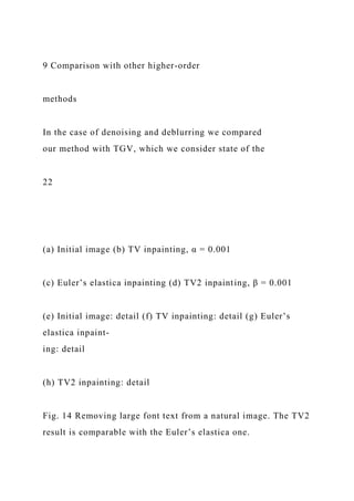
basic synthetic test image is shown in Figure 3.
Fig. 3 Main test image. Resolution: 200× 300 pixels
Our main assessment for the quality of the recon-
struction is the structural similarity index SSIM [73,

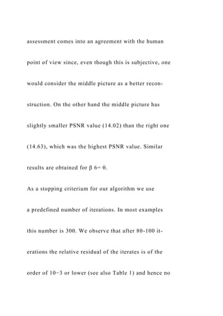
72]. The reason for that choice is that in contrast to
traditional quality measures like the peak signal-to-
noise ratio PSNR, the SSIM index also assesses the
conservation of the structural information of the re-
constructed image. Note that the perfect reconstruc-
tion would have SSIM value equal to 1. A justification
for the choice of SSIM as a good fidelity measure in-
stead of the traditional PSNR can be seen in Figure 4.
The second and the third image are denoising results
with the first order method (β = 0, Gaussian noise,
Variance = 0.1). The middle picture is the one with
the highest SSIM value (0.6595) while the SSIM value
of the right picture is significantly lower (0.4955). This

assessment comes into an agreement with the human
point of view since, even though this is subjective, one
would consider the middle picture as a better recon-
struction. On the other hand the middle picture has
slightly smaller PSNR value (14.02) than the right one
(14.63), which was the highest PSNR value. Similar
results are obtained for β 6= 0.
As a stopping criterium for our algorithm we use
a predefined number of iterations. In most examples
this number is 300. We observe that after 80-100 it-
erations the relative residual of the iterates is of the
order of 10−3 or lower (see also Table 1) and hence no

noticeable change in the iterative solutions is observed
after that.
In the following we shall examine whether the in-
troduction of the higher-order term (β 6= 0) in the
denoising procedure, produces results of higher qual-
ity.
The noise has been produced with MATLAB’s built
in function imnoise.
Figure 5 depicts one denoising example, where the
original image is corrupted with Gaussian noise of
variance 0.005. For better visualisation, we include
the middle row slices of all the reconstructions in Fig-
ure 6. The highest SSIM value for TV denoising is

achieved for α = 0.12 (SSIM=0.8979) while the high-
est one for TV-TV2 is achieved for α = 0.06, β = 0.03
(SSIM=0.9081). This is slightly better than infimal
convolution (SSIM=0.9053). Note, however, that this
optimal combination of α and β in terms of SSIM does
not always correspond to best visual result. In general,
the latter corresponds to a slightly bigger β than the
one chosen by SSIM, see Figure 5(h). Still, for proof of
concept, we prefer to stick with an objective quality
measure and SSIM, in our opinion, is the most reli-
able choice for that matter. In the image of Figure
5(h) the staircasing effect has almost disappeared and
the image is still pleasant to the human eye despite

being slightly more blurry. This slight blur, which is
the price that the method pays for the removal of the
staircasing effect, can be easily and efficiently removed
in post-processing using simple sharpening filters, e.g.
in GIMP. We did that in Figure 5(i), also adjusting the
contrast, and achieve a very good result both visually
and SSIM-wise (0.9463).
16
Fig. 4 Justification for the usage of SSIM index. Best SSIM
value (middle) (SSIM=0.6595, PSNR=14.02) and best PSNR
value (right) (SSIM=0.4955, PSNR=14.63) among reconstructed
images with the first order method (β = 0). The initial
image (left) is contaminated with Gaussian noise of variance
0.5. The better SSIM assessment of the first image agrees more

with the human perception
(a) Clean image, SSIM=1 (b) Noisy image, Gaussian noise, vari-
ance=0.005, SSIM=0.3261
(c) TV denoising, α=0.12, SSIM=0.8979
(d) TGV denoising, SSIM=0.9249 (e) Inf-convolution
denoising, SSIM=
0.9053
(f) TV-TV2 denoising, α=0.06, β=0.03,
SSIM=0.9081
(g) TV2 denoising, β=0.07, SSIM=
0.8988
(h) TV-TV2 denoising, α=0.06, β=0.06,
SSIM=0.8989
(i) TV-TV2 denoising, α=0.06, β=0.06,
SSIM=0.9463, Post-processing: GIMP
sharpening & contrast
Fig. 5 Denoising of an image that has been corrupted with

Gaussian noise of variance 0.005. We chose λ1 = λ2 = 1 for
these implementations
The highest SSIM value is achieved by TGV (0.9249),
delivering a reconstruction of very good quality. How-
ever, TGV converges very slowly to the true solution.
In order to check that, we compute the ground truth
solution (denoted by GT) for the parameters of the
TGV problem that correspond to Figure 5(d), by tak-
ing a large amount of iterations (2000). We check the
GPU time that is needed for the iterates to have a
relative residual
‖uk −GT‖2
‖GT‖2
≤ 10−3

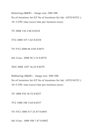
and we do the same for the TV-TV2 example of Figure
5(f). For TGV, it takes 1297 iterations (primal-dual
method [22]) and 36.25 seconds while for TV-TV2 it
takes 86 split Bregman iterations and 4.05 seconds,
17
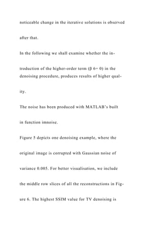
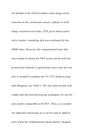
(a) Clean image, SSIM=1 (b) Noisy image, Gaussian noise,
variance=0.005, SSIM=0.3261
(c) TV denoising, α=0.12, SSIM=
0.8979
(d) TGV denoising, SSIM=0.9249 (e) Inf-convolution
denoising,
SSIM=0.9053
(f) TV-TV2 denoising, α=0.06,
β=0.03, SSIM=0.9081

(g) TV2 denoising, β=0.07, SSIM=
0.8988
(h) TV-TV2 denoising, α=0.06,
β=0.06, SSIM=0.8989
(i) TV-TV2 denoising, α=0.06,
β=0.06, SSIM=0.9463,
Post-processing: GIMP sharpening
& contrast
Fig. 6 Corresponding middle row slices of images in Figure 5
see Table 1. That makes our method more suitable for
cases where fast but not necessarily optimal results
are needed, e.g. video processing.
In order to examine the quality of the reconstruc-
tions that are produced from each method as the num-
ber of iteration increases we have plotted in Figure 7

the evolution of SSIM values. In the horizontal axis,
instead of the number of iterations we put the abso-
lute CPU time calculated by the product of the num-
ber of iterations times the CPU time per iteration
as it is seen in Table 1. We observe that, for TGV,
the SSIM value increases gradually with time, while
for the methods solved with split Bregman the image
quality peaks very quickly and then remains almost
constant except for TV where the staircasing appears
in the later iterations.
Next we check how the SSIM and PSNR values
of the restored images behave as a function of the

weighting parameters α and β. In Figure 8 we plot
the results for α = 0, 0.02, 0.04, . . . , 0.3 and β =
0, 0.005, 0.01, . . . , 0.1. The plots suggest that both qual-
ity measures behave in a continuous way and that they
have a global maximum. However, PSNR tends to rate
higher those images that have been processed with a
small value of β or even with β = 0 which is not the
case for SSIM. An explanation for that is that higher
values of β result to a further loss of contrast, see Fig-
ure 9, something that is penalised by the PSNR. The
SSIM index penalises the loss of contrast as well but
it also penalises the creation of the staircasing effect.
This is another indication for the suitability of SSIM

over PNSR. Note also, that the contrast can be re-
covered easily in a post-processing stage while it is
not an easy task to reduce the staircasing effect using
conventional processing tools.
7 Applications in deblurring
In our deblurring implementation T denotes a circular
convolution with a discrete approximation of a Gaus-
sian kernel (σ = 2, size: 11 × 11 pixels). The initial
image is corrupted by additive Gaussian noise of vari-
18
0 0.17 0.5 1.08 1.5 1.89 2.5 3
0.7

0.75
0.8
0.85
0.9
Seconds
S
S
I
M
T V
T V- T V
2
T GV
Inf .C onv .

Fig. 7 Evolution of the SSIM index with absolute CPU time for
the examples of Figure 5. For TV denoising the SSIM value
peaks after 0.17 seconds (0.9130) and the after it drops sharply
since the staircasing appears, see corresponding comments on
[45]. For TV-TV2 the peak appears after 1.08 seconds (0.9103)
and remains essentially constant. The TGV iteration starts
to outperform the methods after 1.89 seconds. This shows the
potential of split Bregman to produce visually satisfactory
results before convergence has occurred, in contrast with the
primal-method.
Fig. 8 Plot of the SSIM and PSNR values of the restored image
as functions of α and β. For display convenience all the
values under 0.85 (SSIM) and 26 (PSNR) were coloured with
dark blue. The dotted cells corresponds to the highest SSIM
(0.9081) and PSNR (32.39) value that were achieved for α =
0.06, β = 0.03 and α = 0.06, β = 0.005 respectively. Note that
the first column in both plots corresponds to TV denoising, (β =
0). The original image was corrupted with Gaussian noise
of variance 0.005
ance 10−4. Let us note here that the optimality con-
dition (5.22) can be solved very fast using fast Fourier

transforms. Deblurring results are shown in Figure 10
and the corresponding middle row slices in Figure 11.
As in the denoising case the introduction of the second
order term with a small weight β decreases noticeably
the staircasing effect, compare Figures (10)(c) and (f).
Moreover, we can achieve better visual results if we in-
crease further the value of β without blurring the im-
age significantly, Figure (10)(g). Infimal convolution
does not give a satisfactory result here, Figure 10(e).
TGV gives again the best qualitative result, Figure
(10)(d), but the computation takes quite a few min-
utes. Even though the time comparison is not com-

pletely fair here (the implementation described in [13]
does not use FFT) it takes a few thousands iterations
for TGV to deblur the image satisfactorily, in compar-
ison with a few hundreds for our TV-TV2 method.
19
Fig. 9 Left: Middle row slices of reconstructed images with α =
0.12, β = 0 (blue colour) and α = 0.12. β = 0.06 (red
colour). Slices of the original image are plotted with black
colour. Right: Detail of the first plot. Even though the higher-
order
method eliminates the staircasing effect, it also results to
further slight loss of contrast
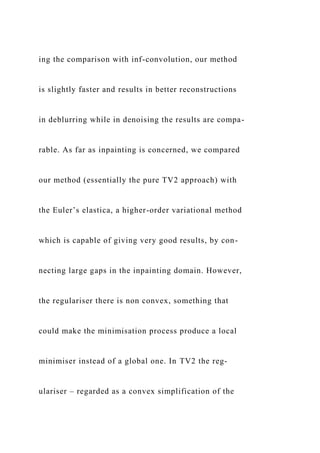
(a) Clean image , SSIM=1 (b) Blurred and noisy image, SSIM=
0.8003
(c) TV deblurring, α=0.006, SSIM=
0.9680

(d) TGV deblurring, SSIM=0.9806 (e) Inf-convolution
deblurring, SSIM=
0.9466
(f) TV-TV2 deblurring, α = 0.004, β =
0.0001, SSIM=0.9739
(g) TV-TV2 deblurring, α = 0.004, β =
0.0002, SSIM=0.9710
(h) TV2 deblurring, β = 0.0012, SSIM=
0.9199
Fig. 10 Deblurring of a blurred (Gaussian kernel of variance σ =
2) and noisy (additive Gaussian noise, variance 10−4)
image. We chose λ1 = 100α, λ2 = 100β for these
implementations.
8 Applications in inpainting
Finally, we present examples for the application of
our TV-TV2 approach to image inpainting. There, the

goal is to reconstruct an image inside a missing part
using information from the intact part. The missing
part is a domain D ⊆ Ω, known as the inpainting do-
main. In this case the operator T applied to an image
u gives
Tu = XΩDu,
where as before XΩD is the characteristic function
of Ω D, the intact part of the image domain. Let us
note here that in cases of a small number of inpainting
domains and a completely noise free and trustable im-
age outside of the missing part, it is preferable to solve
the inpainting problem only inside the holes, see for
20

(a) Clean, image, SSIM=1 (b) Blurred and noisy image,
SSIM=0.8003
(c) TV deblurring, α=0.006, SSIM=
0.9680
(d) TGV deblurring, SSIM=0.9806 (e) Inf-convolution
deblurring,
SSIM=0.9466
(f) TV-TV2 deblurring, α = 0.004,
β = 0.0001, SSIM=0.9739
(g) TV-TV2 deblurring, α = 0.004,
β = 0.0002, SSIM=0.9710
(h) TV2 deblurring, β=0.0012,
SSIM=0.9199
Fig. 11 Corresponding middle row slices of images in Figure 10
example [20]. However, here we would like to keep the
method flexible, such that it includes the case where

there is noise in the known regions as well.
In order to take advantage of the FFT for the opti-
mality condition (5.22) a different splitting technique
to (5.12) is required:
min
u∈ Rn×m
ũ∈ Rn×m
v∈ (Rn×m)
2
w∈ (Rn×m)
3
‖XΩD(u−u0)‖22 + α‖v‖1 + β‖w‖1, (8.1)
such that u = ũ, v = ∈ũ, w = ∈2ũ. We refer the
reader to [56] for the details.
In Figure 12 we compare our method with har-

monic and Euler’s elastica inpainting, see [24, 66]. In
the case of harmonic inpainting the regulariser is the
square of the L2 norm of the gradient
´
Ω
|∇ u|2 dx. In
the case of Euler’s elastica the regulariser is
ˆ
Ω
(
α + β
(
∇ ·
∇ u
|∇ u|
)2)
|∇ u| dx. (8.2)

The minimisation of the Euler’s elastica energy corre-
sponds to the minimisation of the length and curva-
ture of the level lines of the image. Thus, this method
is able to connect large gaps in the inpainting do-
main, see Figure 12(d). However, the term (8.2) is
non-convex and thus difficult to be minimised. In or-
der to implement the Euler’s elastica inpainting we
used the augmented Lagrangian method, proposed in
[66]. There, the leading computational cost per iter-
ation is one linear PDE and a pair of linear PDEs
(solved with FFT as well), in comparison to our ap-
proach which consists of one linear PDE only. That
is why, in Table 1, we do not give absolute computa-

tional times as that would not be fair even more so
because we did not optimise the Euler’s elastica algo-
rithm with respect to the involved parameters.
In Figure 12 we see that, in contrast to harmonic
and TV inpainting, TV2 inpainting is able to connect
big gaps, with the price of a slight blur. Notice that
one has to choose α small or even 0, in order to make
the TV2 dominant, compare Figures 12(e) and (f).
We also observe that in the TV2 case, this ability
to connect large gaps depends on the size and geom-
etry of the inpainting domain, see Figure 13 and also
see [56] for more examples. Deriving sufficient condi-

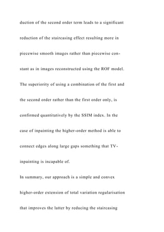
21
(a) Initial image, the gray area de-
notes the inpainting domain D
(b) Harmonic inpainting, α = 0.01 (c) TV inpainting, α = 0.01
(d) Euler’s elastica inpainting (e) TV-TV2 inpainting, α =
0.005,
β = 0.005
(f) TV2 inpainting, β = 0.01
(g) TV2 inpainting – post-processing
with shock filter [2]
Fig. 12 Comparison of different inpainting methods regarding
connectivity across large gaps
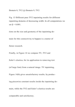
(a) Domain 1 (b) Domain 6 (c) Domain 7 (d) Domain 8 (e)
Domain 9
(f) Domain 1, TV2 (g) Domain 6, TV2 (h) Domain 7, TV2 (i)

Domain 8, TV2 (j) Domain 9, TV2
Fig. 13 Different pure TV2 inpainting results for different
inpainting domains of decreasing width. In all computations we
set β = 0.001.
tions on the size and geometry of the inpainting do-
main for this connectivity to happen is a matter of
future research.
Finally, in Figure 14 we compare TV, TV2 and
Euler’s elastica, for its application to removing text
(of large font) from a natural image. TV inpainting,
Figure 14(b) gives unsatisfactory results, by produc-
ing piecewise constant results inside the inpainting do-
main, while the TV2 and Euler’s elastica results are
comparable and satisfactory.

9 Comparison with other higher-order
methods
In the case of denoising and deblurring we compared
our method with TGV, which we consider state of the
22
(a) Initial image (b) TV inpainting, α = 0.001
(c) Euler’s elastica inpainting (d) TV2 inpainting, β = 0.001
(e) Initial image: detail (f) TV inpainting: detail (g) Euler’s
elastica inpaint-
ing: detail
(h) TV2 inpainting: detail
Fig. 14 Removing large font text from a natural image. The TV2
result is comparable with the Euler’s elastica one.

art method in the field of higher-order image recon-
struction in the variational context. Indeed, in both
image reconstruction tasks, TGV gives better quali-
tative results, something that was confirmed by the
SSIM index. However the computational time that
was needed to obtain the TGV result solved with the
primal-dual method is significantly more than the one
that is needed to compute the TV-TV2 method using
split Bregman, see Table 1. We also showed that with
simple and fast post-processing techniques we can ob-
tain results comparable with TGV. Thus, we consider
our approach interesting as it can be used in applica-
tions when the computational speed matters. Regard-

ing the comparison with inf-convolution, our method
is slightly faster and results in better reconstructions
in deblurring while in denoising the results are compa-
rable. As far as inpainting is concerned, we compared
our method (essentially the pure TV2 approach) with
the Euler’s elastica, a higher-order variational method
which is capable of giving very good results, by con-
necting large gaps in the inpainting domain. However,
the regulariser there is non convex, something that
could make the minimisation process produce a local
minimiser instead of a global one. In TV2 the reg-
ulariser – regarded as a convex simplification of the

Euler’s elastica idea – it has the ability to connect
23
large gaps and the slight blur that is produced can
be reduced by using a shock filter see for example [2,
44] and Figure 12(g). Moreover as we pointed out in
the previous sections, our approach is computationally
less expensive compared to TGV for image denoising
and deblurring and Euler elastica for image inpaint-
ing.
10 Conclusion
We formulate a second order variational problem in
the space of functions of bounded Hessian in the con-

text of convex functions of measures. We prove exis-
tence and uniqueness of minimisers using a relaxation
technique as well as stability. We propose the use of
the split Bregman method for the numerical solution
of the analogue discretised problem. The application
of split Bregman method in our model is quite robust
and is converging after a few iterations. We perform
numerical experiments by denoising images that have
been corrupted with Gaussian noise, deblurring im-
ages that have been convoluted with Gaussian kernels,
as well as in image inpainting.
In the case of denoising and deblurring, the intro-

duction of the second order term leads to a significant
reduction of the staircasing effect resulting more in
piecewise smooth images rather than piecewise con-
stant as in images reconstructed using the ROF model.
The superiority of using a combination of the first and
the second order rather than the first order only, is
confirmed quantitatively by the SSIM index. In the
case of inpainting the higher-order method is able to
connect edges along large gaps something that TV-
inpainting is incapable of.
In summary, our approach is a simple and convex
higher-order extension of total variation regularisation
that improves the latter by reducing the staircasing

effect in image denoising and deblurring, and by more
faithfully respecting the good continuation principle in
image inpainting. It can compete with other higher-
order methods of its kind by giving almost comparable
qualitative results while computing them in a fraction
of time.
As fas as future work is concerned, a (not necessar-
ily rigorous) rule for selecting the parameters α and
β would be useful. Investigating the links with inf-
convolution and spatially dependent regularisation on
our model is also of interest. Moreover, the relation be-
tween the continuum and the discretised model could

be investigated through Γ-convergence arguments, see
[29] and [12]. Finally the characterisation of subgradi-
ents of this approach and the analysis of solutions of
the corresponding PDE flows for different choices of
functions f and g promises to give more insight into
the qualitative properties of this regularisation pro-
cedure. The characterisation of subgradients will also
give more insight to properties of exact solutions of
the minimisation of (1.1) concerning the avoidance of
the staircasing effect.
Acknowledgements The authors acknowledge the finan-
cial support provided by the Cambridge Centre for Analy-
sis (CCA) and the Royal Society International Exchanges
Award IE110314 for the project ”High-order Compressed
Sensing for Medical Imaging”. Further, this publication is

based on work supported by Award No. KUK-I1-007-43 ,
made by King Abdullah University of Science and Technol-
ogy (KAUST). We thank Clarice Poon for providing us with
the Euler’s elastica code. Finally, we would like to thank the
referees for their very useful comments and suggestions that
improved the presentation of the paper.
A Some useful theorems
Proposition A.1. Suppose that g : Rm → R is a continu-
ous function, positively homogeneous of degree 1 and let µ ∈
[M(Ω)]m. Then for every positive measure Radon measure ν
such that µ is absolulely continuous with respect to ν, we have
g(µ) = g
(
µ
ν
)
ν.
Moreover, if g is a convex function, then g : [M(Ω)]m →
M(Ω) is a convex function as well.

Proof. Since µ � ν, we have that |µ| � ν. Using the fact
that g is positively homogeneous and the fact that |µ|/ν is
a positive function, we get
g(µ) = g
(
µ
|µ|
)
|µ| = g
(
µ
|µ|
)
|µ|
ν
ν = g

(
µ
|µ|
|µ|
ν
)
ν = g
(
µ
ν
)
ν.
Assuming that g is convex and using the first part of the
proposition we get for 0 ≤ λ ≤ 1, µ, ν ∈ [M(Ω)]m:
g(λµ + (1 −λ)ν) = g
(
λµ + (1 −λ)ν
|λµ + (1 −λ)ν|

)
|λµ + (1 −λ)ν|
= g
(
λµ + (1 −λ)ν
|µ| + |ν|
)
(|µ| + |ν|)
= g
(
λ
µ
|µ| + |ν|
+ (1 −λ)
ν

|µ| + |ν|
)
(|µ| + |ν|)
≤ λg
(
µ
|µ| + |ν|
)
(|µ| + |ν|) + (1 −λ)g
(
ν
|µ| + |ν|
)
(|µ| + |ν|)
= λg

(
µ
|µ|
)
|µ| + (1 −λ)g
(
ν
|ν|
)
|ν|
= λg(µ) + (1 −λ)g(ν).
The following theorem which is a special case of a the-
orem that was proved in [19] and can be also found in [4]
establishes the lower semicontinuity of convex functionals of
measures with respect to the weak∗ convergence.
Theorem A.2 (Buttazzo-Freddi, 1991). Let Ω be an open
subset of Rn, ν, (νk)k∈ N be Rm-valued finite Radon measures

and µ, (µk)k∈ N be positive Radon measures in Ω. Let g : Rm →
R be a convex function and suppose that νk → ν and µk →
µ weakly∗ in Ω. Consider the Lebesgue decompositions ν =
(ν/µ)µ + νs, νk = (νk/µk)µk + ν
s
k
, k ∈ N. Then
ˆ
Ω
g
(
ν
µ
(x)
)
dµ(x) +
ˆ
Ω

g∞
(
νs
|νs|
(x)
)
d|νs|(x) ≤
lim inf
k→∞
ˆ
Ω
g
(
νk
µk
(x)

)
dµk(x) +
ˆ
Ω
g∞
(
νs
k
|νs
k
|
(x)
)
d|νsk|(x).
24

Denoising (B&W) – Image size: 200×300
No of iterations for GT No of iterations for ‖uk −GT‖2/‖GT‖2 ≤
10−3 CPU time (secs) time per iteration (secs)
TV 2000 136 2.86 0.0210
TV2 2000 107 3.62 0.0338
TV-TV2 2000 86 4.05 0.0471
Inf.-Conv. 2000 58 3.33 0.0574
TGV 2000 1297 36.25 0.0279
Deblurring (B&W) – Image size: 200×300
No of iterations for GT No of iterations for ‖uk −GT‖2/‖GT‖2 ≤
10−2 CPU time (secs) time per iteration (secs)
TV 1000 478 10.72 0.0257
TV2 1000 108 3.64 0.0337
TV-TV2 1000 517 25.47 0.0493
Inf.-Conv. 1000 108 7.47 0.0692

TGV CPU time more than 10 minutes – see relevant comment in
Section 7 1.22
Inpainting (Colour) – Image size: 375×500
No of iterations for ‖uk −uk−1‖2/‖uk−1‖2 ≤ 8 · 10−3 CPU time
(secs) time per iteration (secs)
TV 88 26.67 0.3031
TV2 103 46.34 0.4499
E.e. CPU time more than 10 minutes – see relevant comment in
Section 8
Table 1 Computational times for the examples of Figures 5, 10
and 14. For the denoising and deblurring examples we
computed a ground true solution (GT) for every method by
taking a large number of iterations and record the number of
iterations and CPU time it takes for the relative residual of the
iterates and the ground true solution to fall below a certain
threshold. For the inpainting, we give the number of iterations
and CPU time it took to compute the solutions shown
in Figure 14, where we chose as a stopping criterium a small
relative residual of the iterates. The TGV examples were

computed using σ = τ = 0.25 in the primal-dual method
described in [13]. The implementation was done using
MATLAB
(2011) in a Macbook 10.7.3, 2.4 GHz Intel Core 2 Duo and 2
GB of memory
In particular, if µ = µk = Ln for all k ∈ N then according
to the definition (2.1) the above inequality can be written as
follows:
g(ν)(Ω) ≤ lim inf
k→∞
g(νk)(Ω).
The following theorem is a special case of Theorem 2.3
in [32].
Theorem A.3 (Demengel-Temam, 1984). Suppose that Ω ⊆
Rn is open, with Lipschitz boundary and let g be a convex
function from Rn×n to R with at most linear growth at in-
finity. Then for every u ∈ BH(Ω) there exists a sequence
(uk)k∈ N ⊆ C∞(Ω) ∩W2,1(Ω) such that
‖uk −u‖L1(Ω) → 0, |D

2uk|(Ω) →|D2u|(Ω),
g(D2uk)(Ω) → g(D2u)(Ω), as k →∞.
Lemma A.4 (Kronecker’s lemma). Suppose that (an)n∈ N
and (bn)n∈ N are two sequences of real numbers such that∑∞
n=1
an < ∞ and 0 < b1 ≤ b2 ≤ . . . with bn →∞. Then
1
bn
n∑
k=1
bkak → 0, as n →∞.
In particular, if (cn)n∈ N is a decreasing positive real sequence
such that
∑∞
n=1

c2n < ∞, then
cn
n∑
k=1
ck → 0, as n →∞.
References
1. R. Acar and C. R. Vogel. Analysis of bounded varia-
tion penalty methods for ill-posed problems. In Inverse
Problems, pages 1217–1229, 1994.
2. L. Alvarez and L. Mazorra. Signal and image restora-
tion using shock filters and anisotropic diffusion. SIAM
Journal on Numerical Analysis, pages 590–605, 1994.
3. M. Amar and V. Cicco. Relaxation of quasi-convex inte-
grals of arbitrary order. Proceedings of the Royal Society
of Edinburgh: Section A Mathematics, 124(05):927–946,
1994.
4. L. Ambrosio, N. Fusco, and D. Pallara. Functions of

bounded variation and free discontinuity problems. Oxford
University Press, USA, 2000.
5. M. Benning. Singular Regularization of Inverse Problems.
PhD thesis, 2011.
6. M. Benning, C. Brune, M. Burger, and J. Müller.
Higher-order TV methods – Enhancement via Bregman
iteration. UCLA CAM Report 12-04, 2012.
7. M. Benning and M. Burger. Error estimates for general
fidelities. Electronic Transactions on Numerical Analysis,
38(44-68):77, 2011.
8. M. Bergounioux and L. Piffet. A second-order model
for image denoising. Set Valued Anal. Variational Anal,
18(3-4):277–306, 2010.
9. A. Bertozzi, S. Esedoglu, and A. Gillette. Analysis of a
two-scale cahn-hilliard model for binary image inpaint-
ing. Multiscale Modeling and Simulation, 6(3):913–936,
2008.
10. A. L. Bertozzi and J. B. Greer. Low-curvature image
simplifiers: Global regularity of smooth solutions and

25
laplacian limiting schemes. Communications on Pure and
Applied Mathematics, 57(6):764–790, 2004.
11. S. Boyd, N. Parikh, E. Chu, B. Peleato, and J. Eckstein.
Distributed optimization and statistical learning via the
alternating direction method of multipliers. Foundations
and Trends in Machine Learning, 3(1):1–122, 2011.
12. A. Braides. Γ -convergence for beginners. Oxford lecture
series in mathematics and its applications, 2002.
13. K. Bredies. Recovering piecewise smooth multichannel
images by minimization of convex functionals with total
generalized variation penalty. preprint, 2012.
14. K. Bredies, K. Kunisch, and T. Pock. Total generalized
variation. SIAM Journal on Imaging Sciences, 3:1–42,
2009.
15. K. Bredies and T. Valkonen. Inverse problems with

second-order total generalized variation constraints. In
Proceedings of SampTA 2011 - 9th International Con-
ference on Sampling Theory and Applications, Singapore,
2011.
16. M. Burger, L. He, and C. Schönlieb. Cahn-hilliard
inpainting and a generalization for grayvalue images.
SIAM J. Imaging Sci., 2(4):1129–1167, 2009.
17. M. Burger and S. Osher. Convergence rates of convex
variational regularization. Inverse problems, 20:1411,
2004.
18. M. Burger, E. Resmerita, and L. He. Error estimation
for bregman iterations and inverse scale space methods
in image restoration. Computing, 81(2):109–135, 2007.
19. G. Buttazzo and L. Freddi. Functionals defined on
measures and applications to non equi-uniformly ellip-
tic problems. Annali di Matematica Pura ed Applicata,
159(1):133–149, 1991.
20. J. Cai, R. Chan, and Z. Shen. A framelet-based image
inpainting algorithm. Applied and Computational Har-

monic Analysis, 24(2):131–149, 2008.
21. A. Chambolle and P. Lions. Image recovery via to-
tal variation minimization and related problems. Nu-
merische Mathematik, 76:167–188, 1997.
22. A. Chambolle and T. Pock. A first-order primal-dual
algorithm for convex problems with applications to
imaging. Journal of Mathematical Imaging and Vision,
40(1):120–145, 2011.
23. T. Chan and S. Esedoglu. Aspects of total variation
regularized L1 function approximation. SIAM Journal
on Applied Mathematics, pages 1817–1837, 2005.
24. T. Chan, S. Kang, and J. Shen. Euler’s elastica and
curvature-based inpainting. SIAM Journal on Applied
Mathematics, 63(2):564–592, 2002.
25. T. Chan, A. Marquina, and P. Mulet. High-order total
variation-based image restoration. SIAM J. Sci. Com-
put., 22(2):503–516, 2001.
26. T. F. Chan, E. S., and F. Park. Image decomposi-
tion combining staircase reduction and texture extrac-

tion. J. Visual Communication and Image Representation,
18(6):464–486, 2007.
27. P. Charbonnier, L. Blanc-Fraud, G. Aubert, and
M. Barlaud. Two deterministic half-quadratic regu-
larization algorithms for computed imaging. In ICIP
(2)’94, pages 168–172, 1994.
28. P. Combettes, V. Wajs, et al. Signal recovery by proxi-
mal forward-backward splitting. Multiscale Modeling and
Simulation, 4(4):1168–1200, 2006.
29. G. Dal Maso. Introduction to Γ -convergence. Birkhauser,
1993.
30. G. Dal Maso, I. Fonseca, G. Leoni, and M. Morini. A
higher order model for image restoration: the one di-
mensional case. SIAM J. Math. Anal, 40(6):2351–2391,
2009.
31. F. Demengel. Fonctions à hessian borné. Ann. Inst.
Fourier, 34:155–190, 1985.
32. F. Demengel and R. Temam. Convex functions of
a measure and applications. Indiana Univ. Math. J.,

33:673–709, 1984.
33. S. Didas, J. Weickert, and B. Burgeth. Properties of
higher order nonlinear diffusion filtering. J. Math. Imag-
ing Vis., 35:208–226, 2009.
34. Y. Dong, M. Hintermüller, F. Knoll, and R. Stollberger.
Total variation denoising with spatially dependent reg-
ularization. In ISMRM 18th Annual Scientific Meeting
and Exhibition Proceedings, page 5088, 2010.
35. V. Duval, J. Aujol, and Y. Gousseau. The TV-L1 model:
a geometric point of view. SIAM journal on multiscale
modeling and simulation, 8(1):154–189, 2009.
36. J. Eckstein. Splitting methods for monotone operators with
applications to parallel optimisation. PhD thesis, 1989.
37. I. Ekeland and R. Témam. Convex Analysis and Varia-
tional Problems. Classics in Applied Mathematics. Soci-
ety for Industrial and Applied Mathematics, 1999.
38. E. Esser, X. Zhang, and T. Chan. A general framework
for a class of first order primal-dual algorithms for tv
minimization. UCLA CAM Report 09-67, 2009.

39. L. Evans. Partial Differential Equations, volume 19 of
Graduate Studies in Mathematics, Second Edition. Amer-
ican Mathematical Society,, 2010.
40. X. Feng and A. Prohl. Analysis of total vari-
ation flow and its finite element approximations.
ESAIM-Mathematical Modelling and Numerical Analysis,
37(3):533, 2003.
41. K. Frick, P. Marnitz, and A. Munk. Statistical
multiresolution estimation in imaging: Fundamental
concepts and algorithmic framework. Arxiv preprint
arXiv:1101.4373, 2011.
42. C. Frohn-Schauf, S. Henn, and K. Witsch. Nonlinear
multigrid methods for total variation image denoising.
Computing and Visualization in Science, 7(3):199–206,
2004.
43. D. Gabay. Chapter IX, Applications of the method of
multipliers to variational inequalities. In M. Fortin and
R. Glowinski, editors, Augmented Lagrangian Methods:
Applications to the Numerical

Noname manuscript No.(will be inserted by the editor)A c.docx

Noname manuscript No.(will be inserted by the editor)A c.docx

More Related Content

Similar to Noname manuscript No.(will be inserted by the editor)A c.docx

More from henrymartin15260

Recently uploaded

Noname manuscript No.(will be inserted by the editor)A c.docx