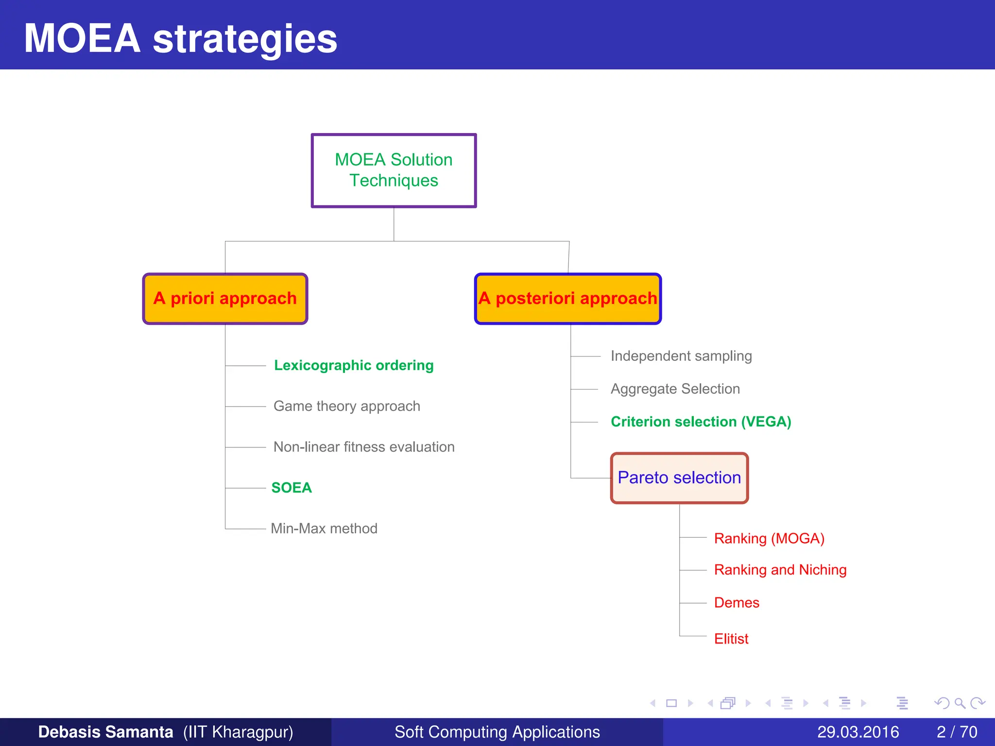
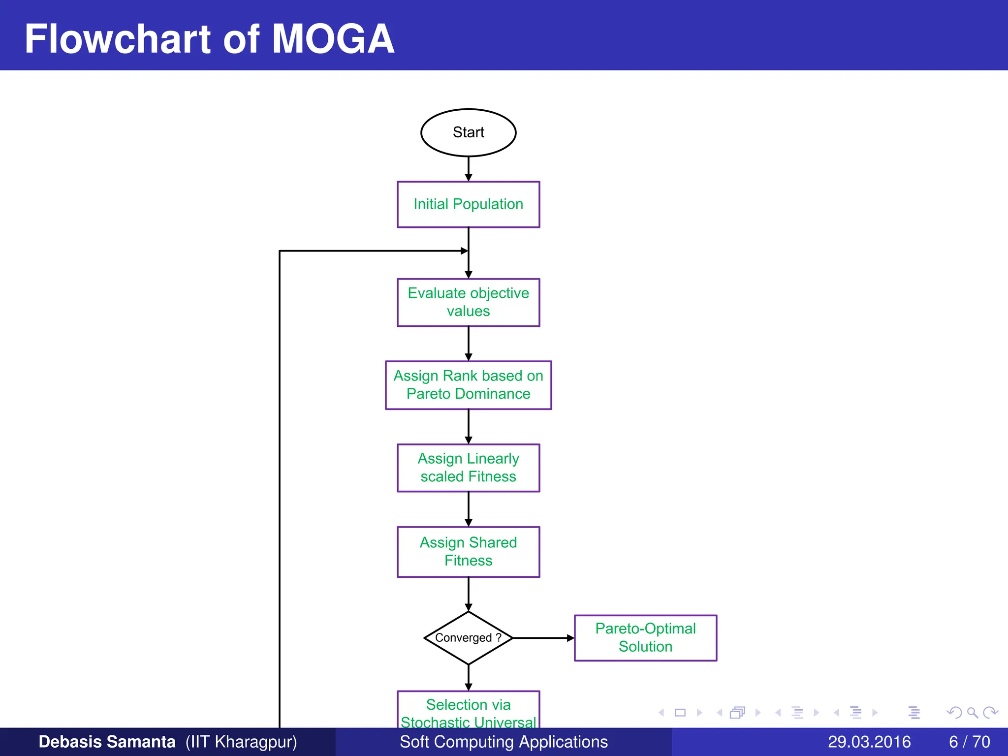
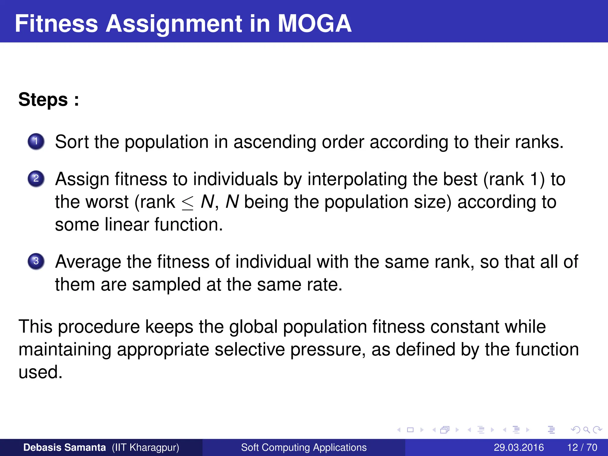
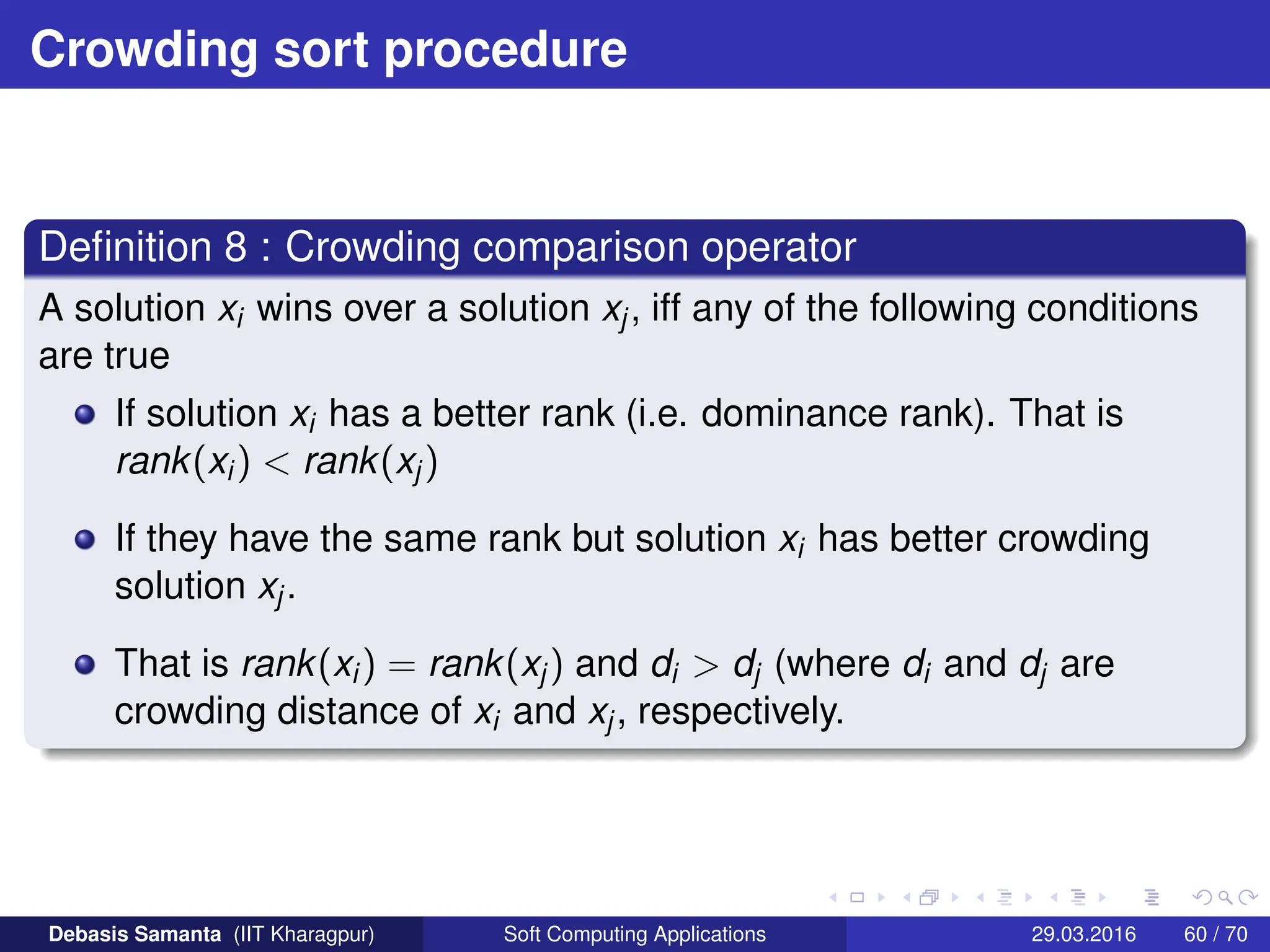
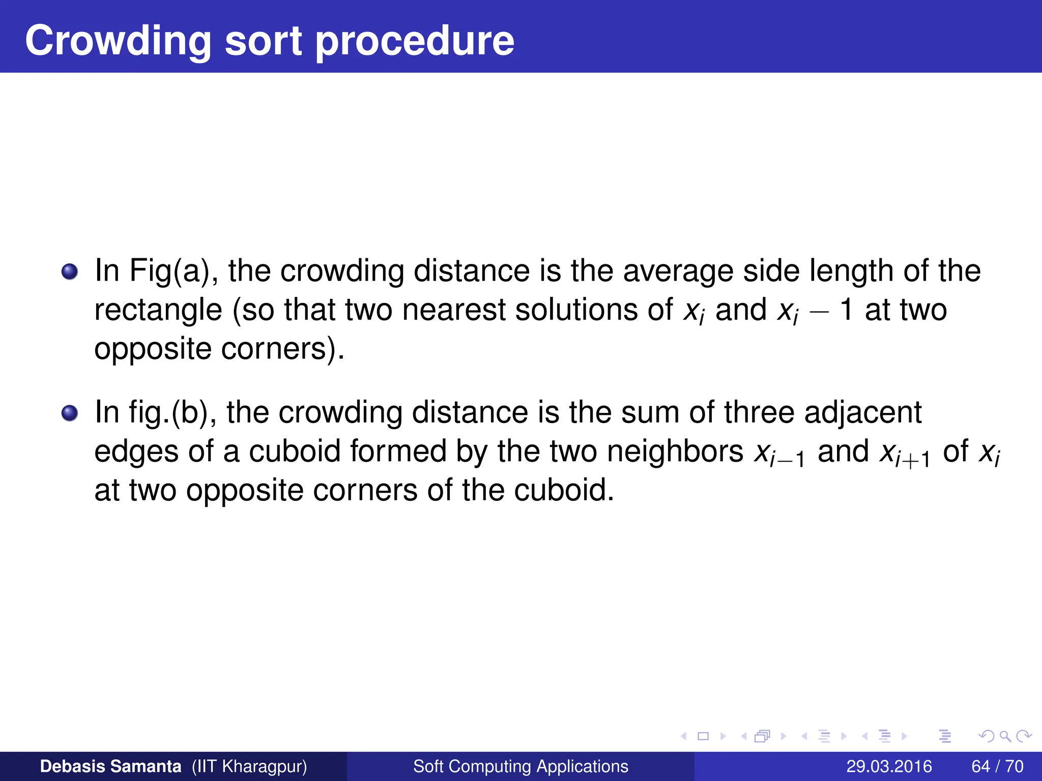
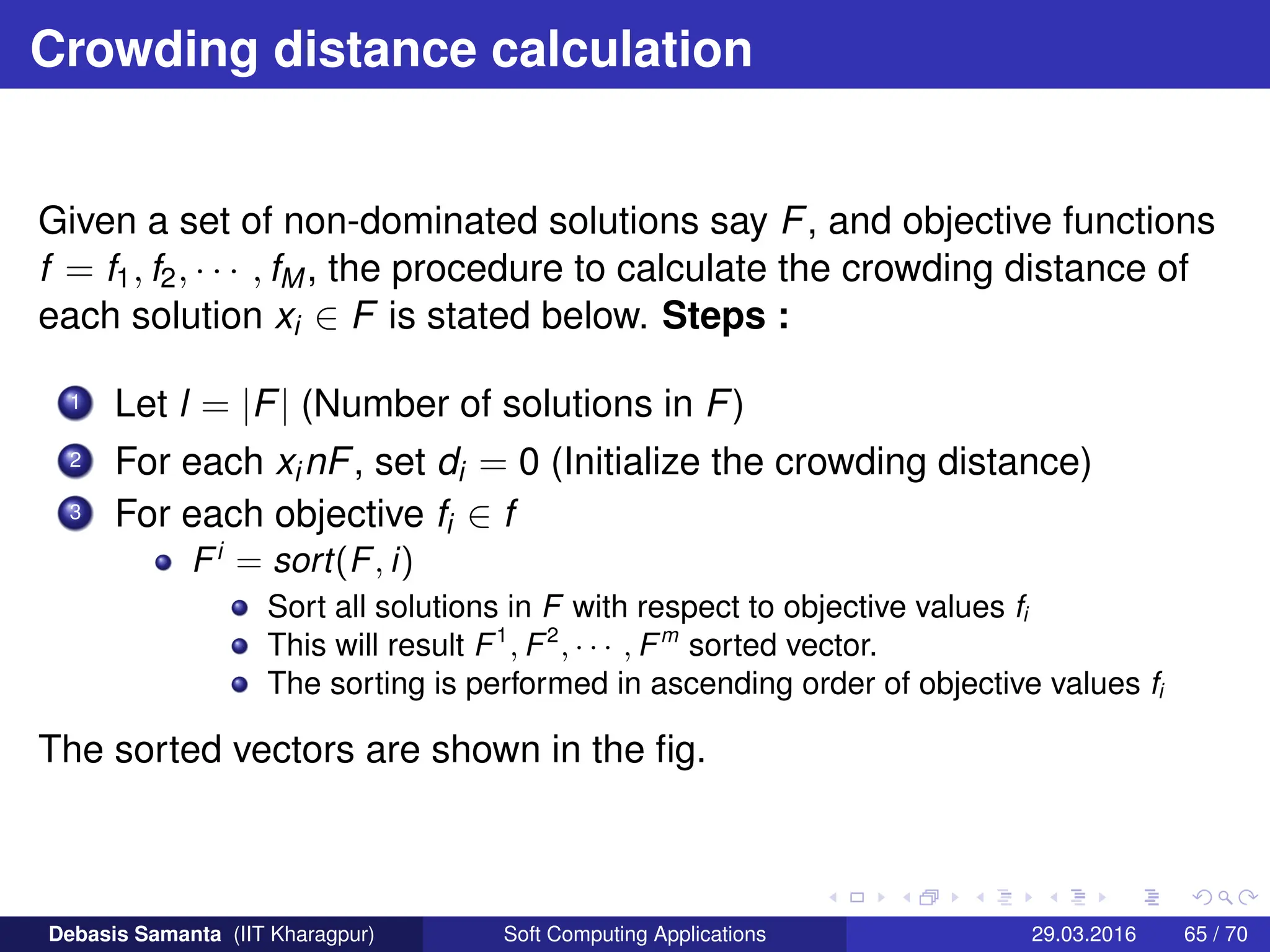
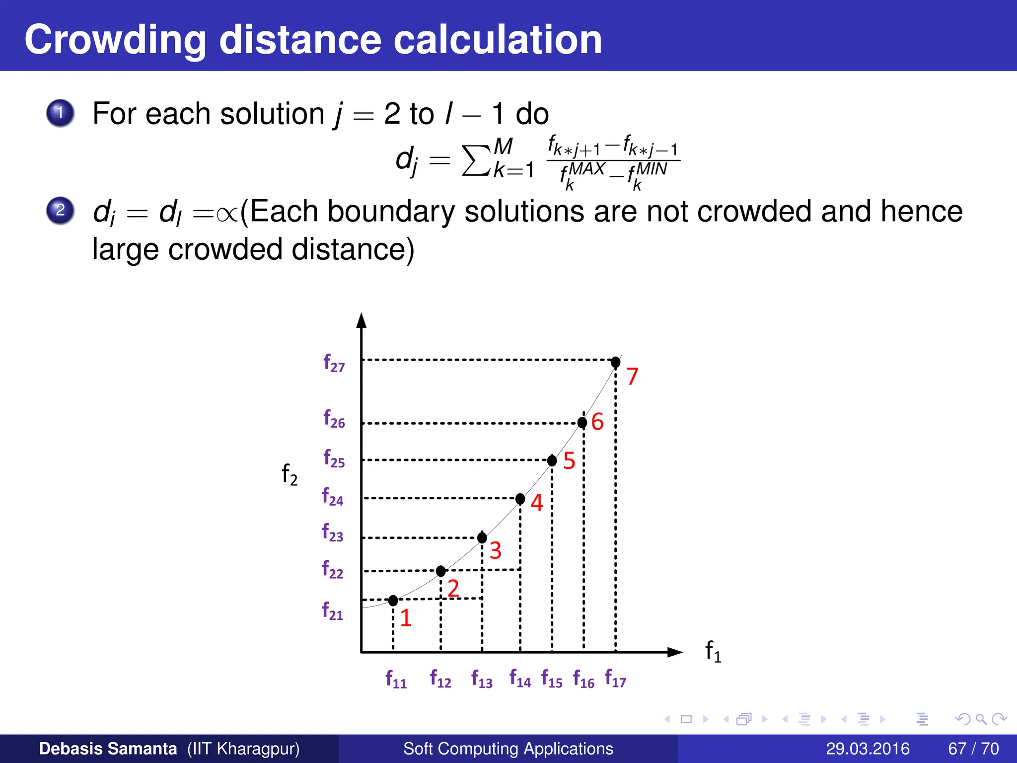
This document summarizes several multi-objective evolutionary algorithm techniques for solving multi-objective optimization problems (MOOPs). It begins by describing the MOGA (Multi-Objective Genetic Algorithm) approach, including dominance-based ranking, linearized fitness assignment, and fitness averaging. It then explains the NPGA (Niched Pareto Genetic Algorithm) technique which uses a Pareto tournament selection scheme and niche sharing to maintain diversity. Finally, it briefly introduces the NSGA (Non-dominated Sorting Genetic Algorithm) method based on non-dominated sorting and a niche approach.


![Niched Pareto Genetic Algorithm (NPGA)
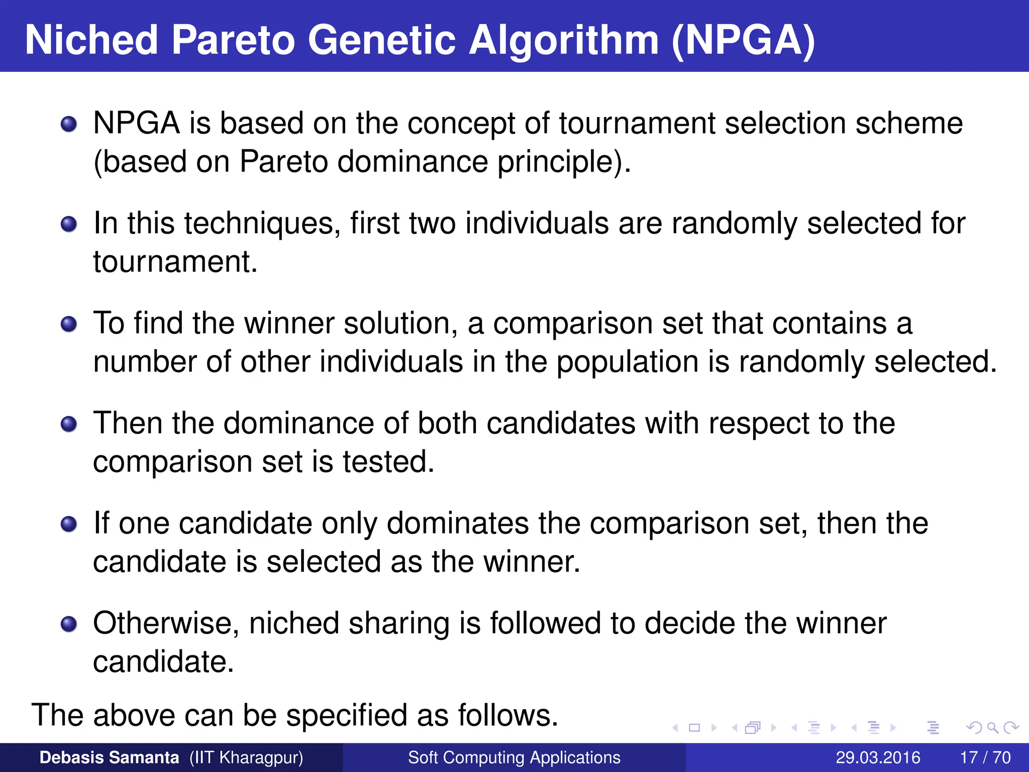
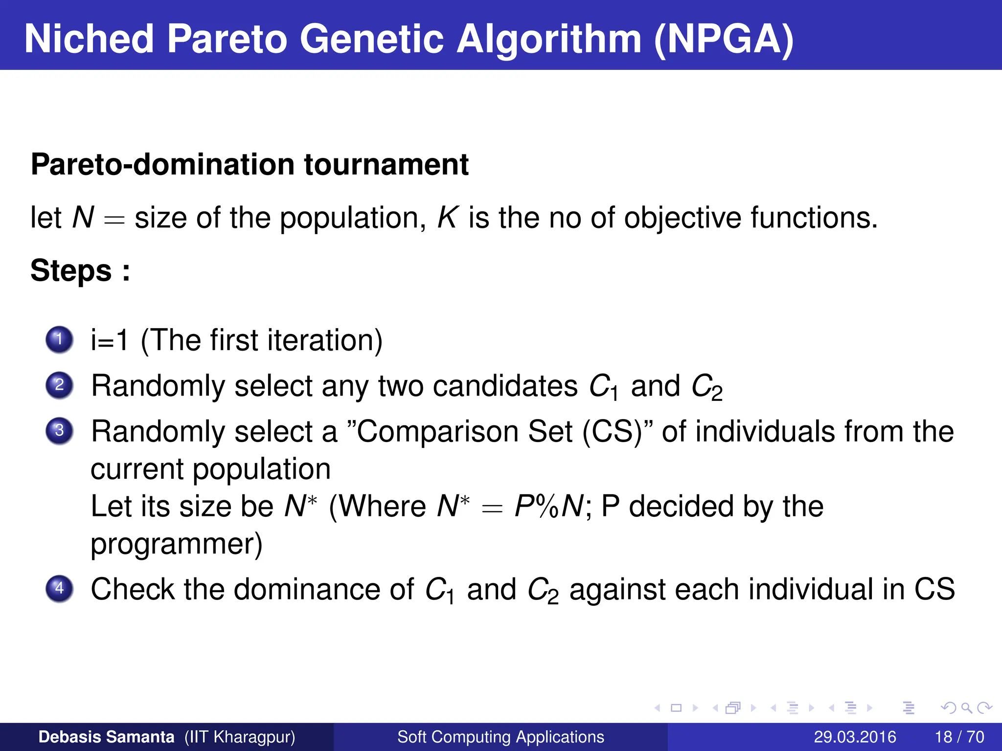
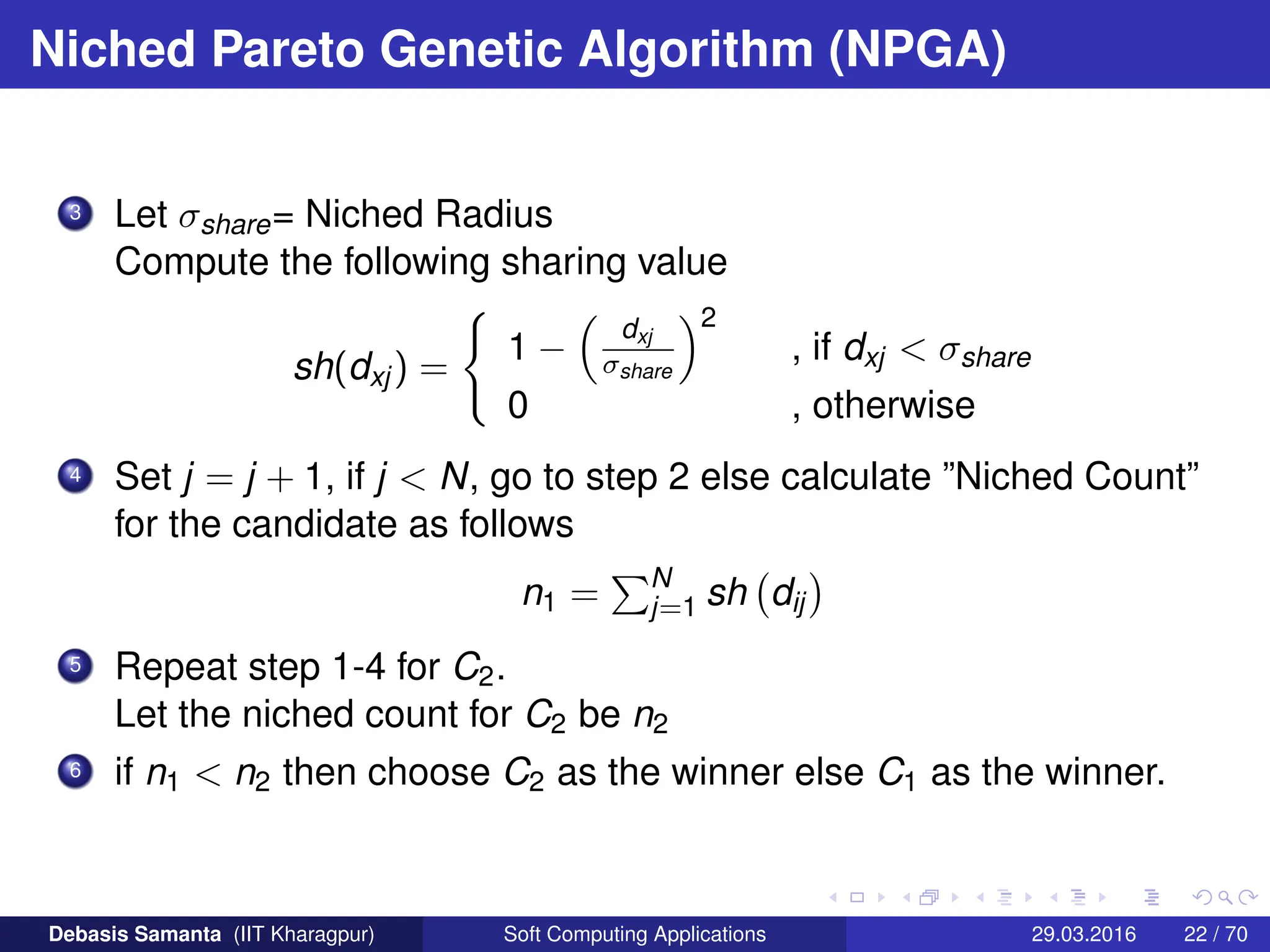
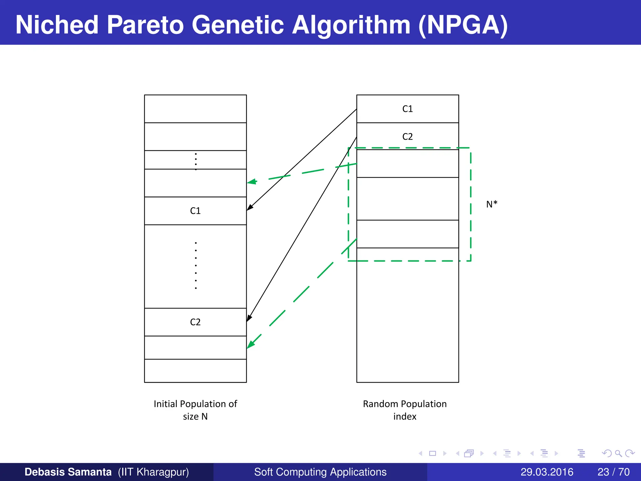
This approach proposed by Horn and Nafploitis [1993]. The approach
is based on tournament scheme and Pareto dominance. In this
approach, a comparison was made among a number of individuals
(typically 10%) to determine the dominance. When both competitors
are dominated or non-dominated (that is, there is a tie) the result of the
tournament is decided through fitness sharing (also called equivalent
class sharing)
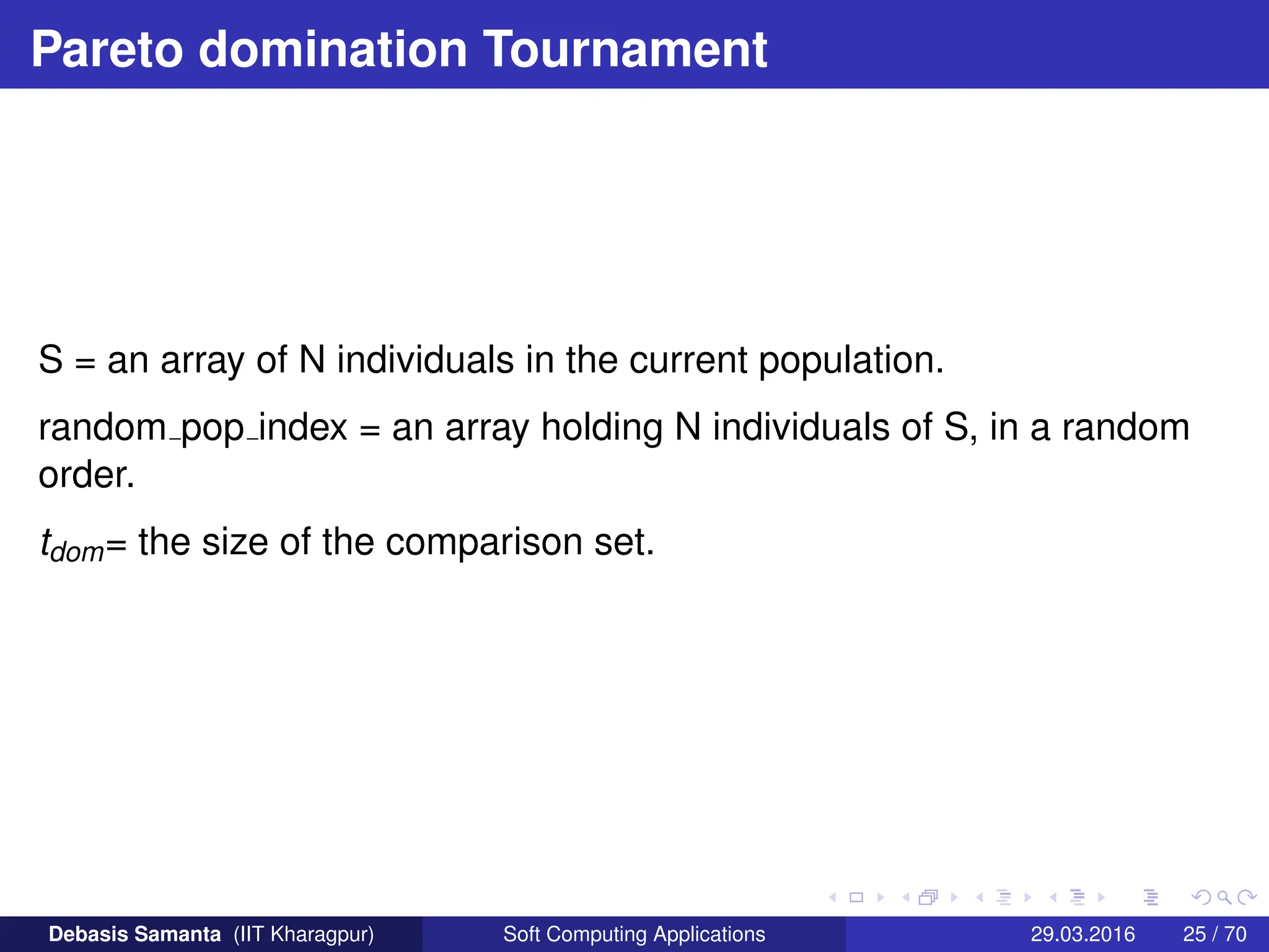
The pseudo code for Pareto domination tournament assuming that all
of the objectives are to be maximized is presented below. Let us
consider the following.
Debasis Samanta (IIT Kharagpur) Soft Computing Applications 29.03.2016 24 / 70](https://image.slidesharecdn.com/newfile-240123043838-217f3e6c/75/new-file-best-book-from-the-university-pdf-24-2048.jpg)

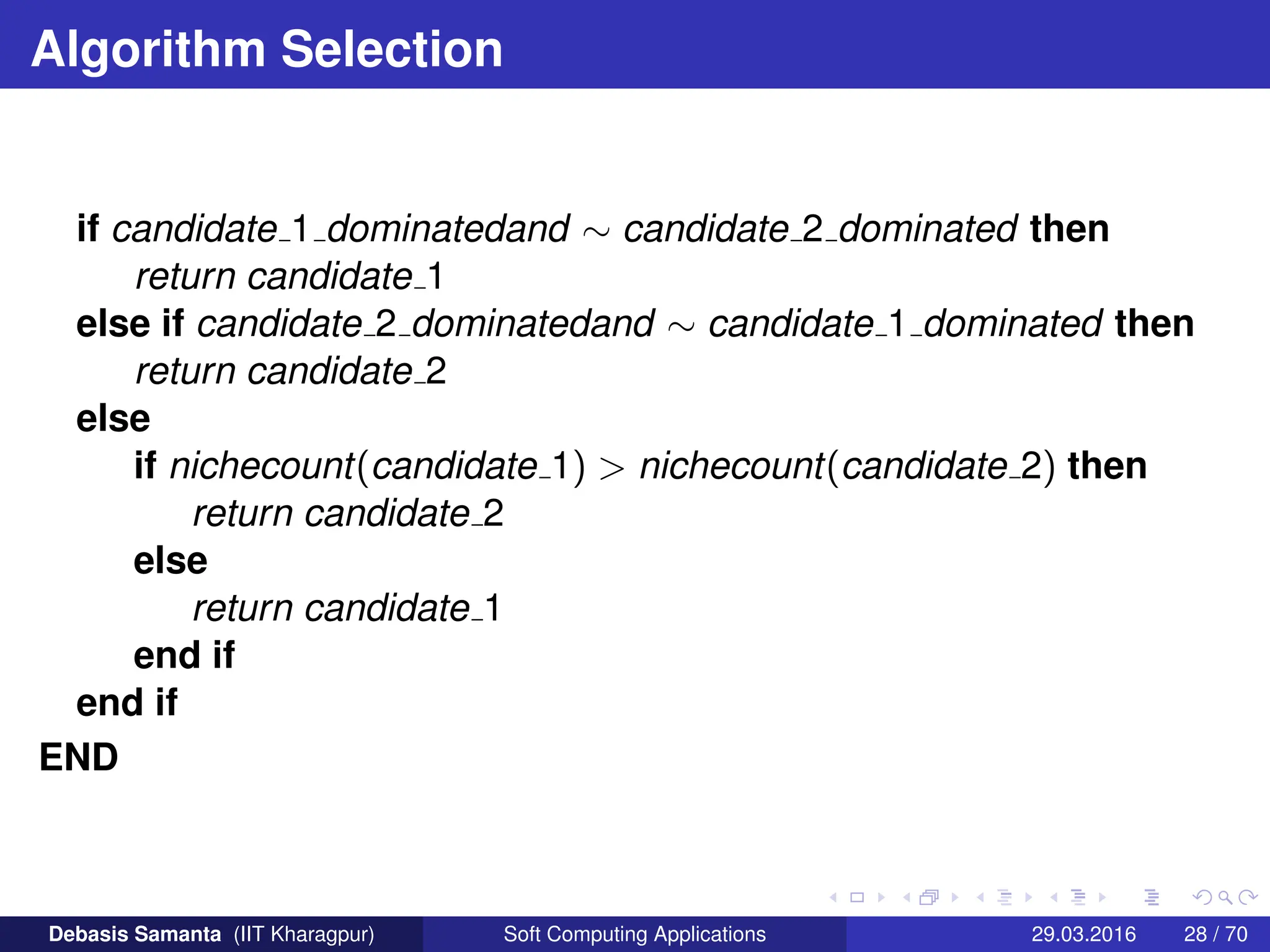
![Algorithm Selection
This algorithm returns an individual from the current population S.
Begin
shuffle(random pop index)
candidate 1 = random pop index[1];
candidate 2 = random pop index[2];
candidate 1 dominated = F;
candidate 2 dominated = F;
for comparison set index = 3 to tdom + 3 do
comparison individual = random pop index[comparison set index];
if s[comparison set index]dominatess[candidate 1] then
candidate 1 dominated = TRUE;
end if
if s[comparison set index]dominatess[candidate 2] then
candidate 2 dominated = TRUE;
end if
end for
Debasis Samanta (IIT Kharagpur) Soft Computing Applications 29.03.2016 27 / 70](https://image.slidesharecdn.com/newfile-240123043838-217f3e6c/75/new-file-best-book-from-the-university-pdf-27-2048.jpg)
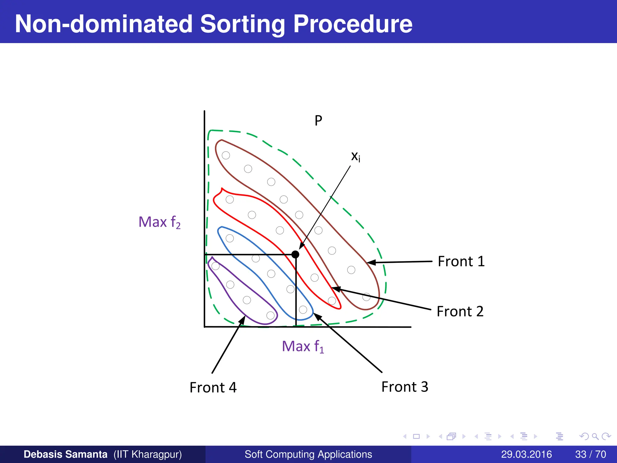
![Non-dominated Sorting Procedure
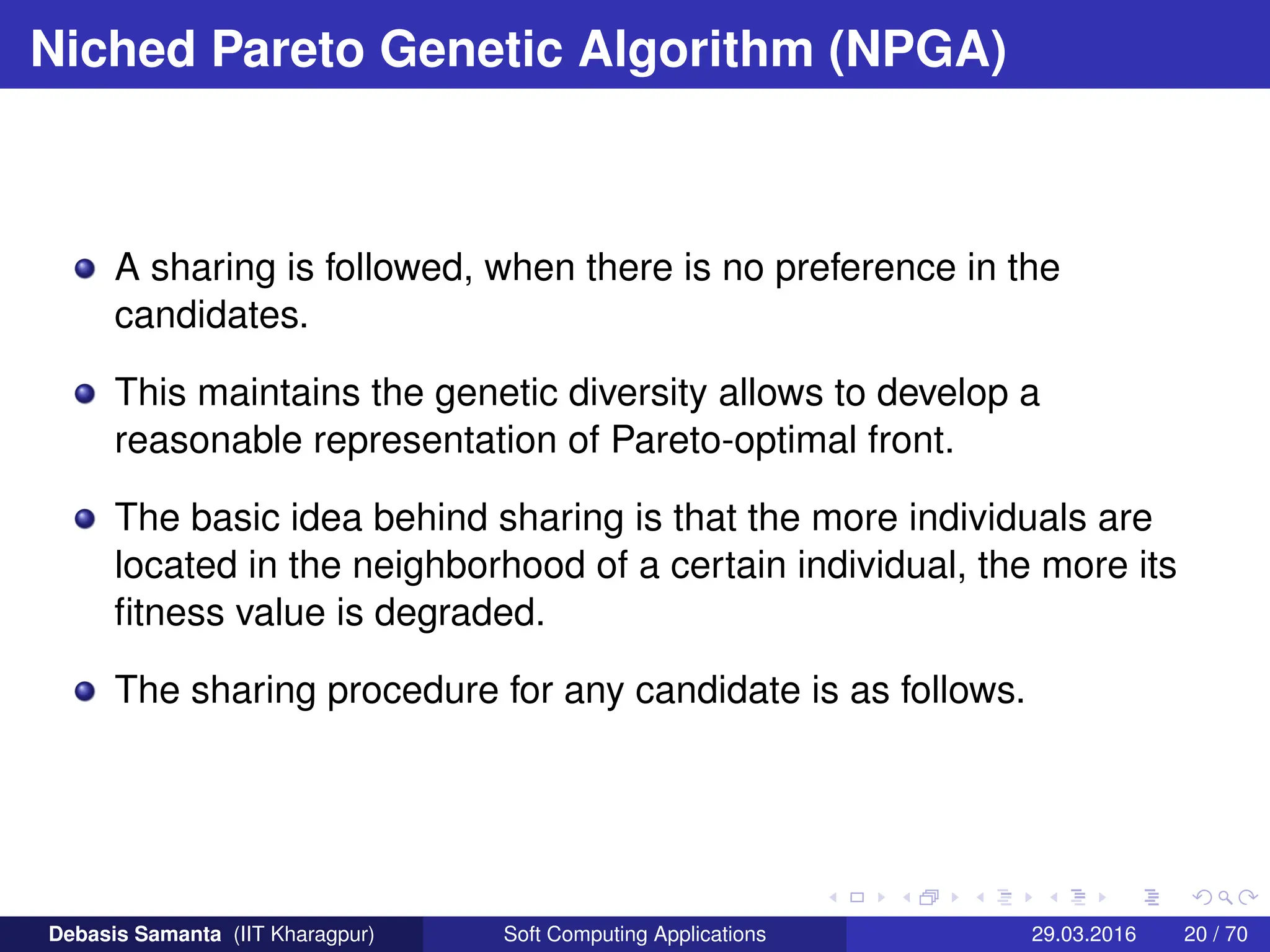
Steps :
1 For each xi ∈ P do
1 For all xj 6= xi and xj ∈ P
If xi ≤ xj (i.e. if xi ) dominates xj
then si = si ∪ xj
else if xj ≤ xi then ni = ni + 1
2 If ni = 0, keep xi in P1 (the first front). Set a front counter K = 1
2 [INITIALIZATION]
For each xi ∈ P, ni = 0 and Si = φ
−− This completes the finding of first front −−
Debasis Samanta (IIT Kharagpur) Soft Computing Applications 29.03.2016 34 / 70](https://image.slidesharecdn.com/newfile-240123043838-217f3e6c/75/new-file-best-book-from-the-university-pdf-34-2048.jpg)
![Non-dominated Sorting Procedure
−− To find other fronts −−
3 While Pk = φ do
1 [Initialize] Q = φ (for sorting next non-dominated solutions)
2 For each xi ∈ Pk and For each xj ∈ Si do
Update nj = nj − 1
If nj = 0 then xj in Q Else Q = Q ∪ xj
3 Set k = k + 1 and Pk = Q (Go for the next front)
Debasis Samanta (IIT Kharagpur) Soft Computing Applications 29.03.2016 35 / 70](https://image.slidesharecdn.com/newfile-240123043838-217f3e6c/75/new-file-best-book-from-the-university-pdf-35-2048.jpg)
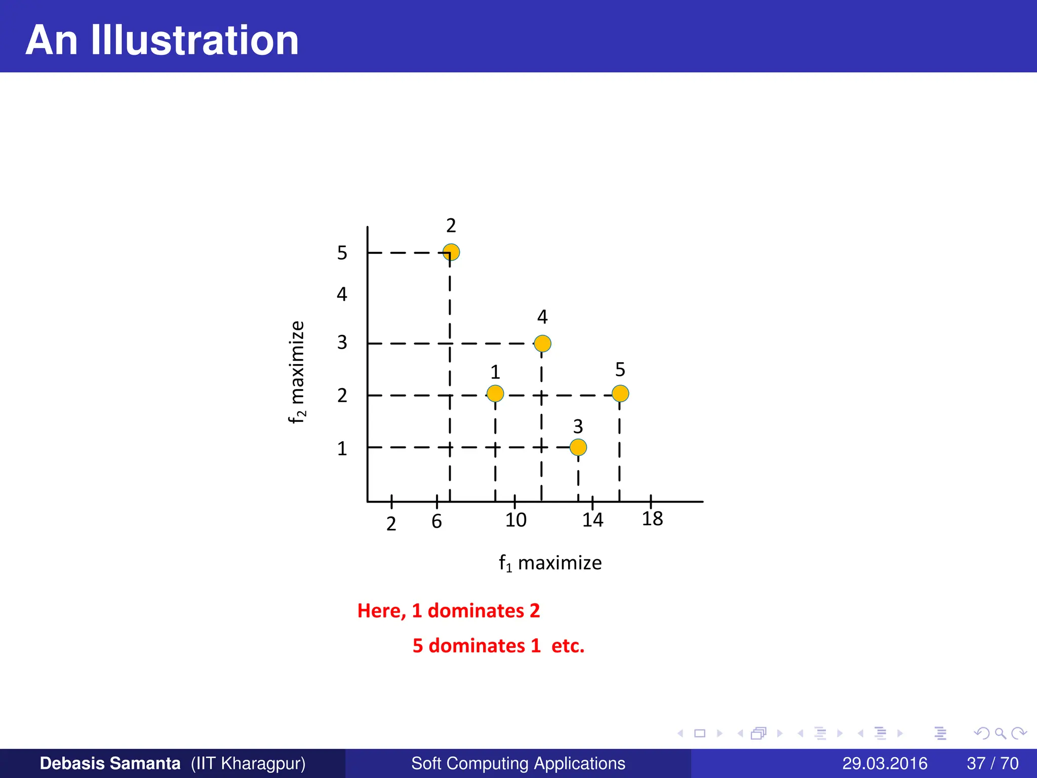
![Non-dominated Sorting Procedure
Three non-dominated fronts as shown.
The solutions in the front [3, 5] are the best, follows by solutions
[1, 4].
Finally, solution [2] belongs to the worst non-dominated front.
Thus, the ordering of solutions in terms of their non-domination
level is : [3, 5], [1, 4], [2]
Debasis Samanta (IIT Kharagpur) Soft Computing Applications 29.03.2016 38 / 70](https://image.slidesharecdn.com/newfile-240123043838-217f3e6c/75/new-file-best-book-from-the-university-pdf-38-2048.jpg)


![[IJCT-V3I2P31] Authors: Amarbir Singh](https://cdn.slidesharecdn.com/ss_thumbnails/ijct-v3i2p31-160609071410-thumbnail.jpg?width=640&height=640&fit=bounds)