natural language processing

1. Chapter 6:
Statistical Inference: n-gram
Models over Sparse Data
1

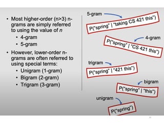
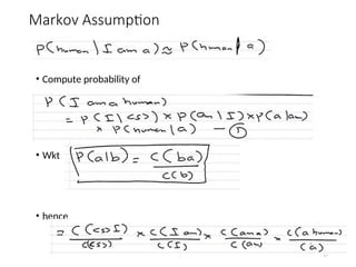
2. Overview
• Statistical Inference consists of taking some data (generated
in accordance with some unknown probability distribution)
and then making some inferences about this distribution.
• There are three issues to consider:
• Dividing the training data into equivalence classes
• Finding a good statistical estimator for each equivalence class
• Combining multiple estimators
2

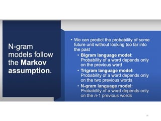
3. Basic Idea of statistical inference:
• Examine short sequences of words
• How likely is each sequence?
• “Markov Assumption” – word is affected only by its “prior local
context” (last few words)

4. Possible Applications:
•OCR / Voice recognition – resolve ambiguity
•Spelling correction
•Machine translation
•Confirming the author of a newly discovered work
•“Shannon game”
• Predict the next word, given (n-1) previous words
• Determine probability of different sequences by
examining training corpus

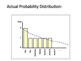
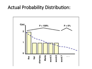
5. Forming Equivalence Classes (Bins)
• Classification : to predict the target feature on the basis of various
classificatory features.
• When doing this, we effectively divide the data into equivalence classes
that share values for certain of the classificatory features, and use this
equivalence classing to help predict the value of the target feature on
new pieces of data.
• This means that we are tacitly making independence assumptions: the
data either does not depend on other features, or the dependence is
sufficiently minor that we hope that we can neglect it without doing too
much harm.
• “n-gram” = sequence of n words
• bigram
• trigram
• four-gram

6. Reliability vs. discrimination
•Dividing the data into many bins gives us greater
Discrimination.
•Going against this is the problem that if we use a lot
of bins then a particular bin may contain no or a
very small number of training instances, and then
we will not be able to do statistically reliable
estimation of the target feature for that bin.
•Finding equivalence classes that are a good
compromise between these two criteria is our first
goal.
6

7. Reliability vs. Discrimination
• larger n: more information about the context of the specific
instance (greater discrimination)
• smaller n: more instances in training data, better statistical
estimates (more reliability)

8. Reliability vs. Discrimination
“large green ___________”
tree? mountain? frog? car?
“swallowed the large green ________”
pill? broccoli?

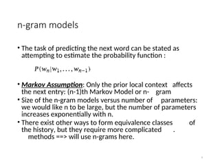
9. n-gram models
• The task of predicting the next word can be stated as
attempting to estimate the probability function :
• Markov Assumption: Only the prior local context affects
the next entry: (n-1)th Markov Model or n- gram
• Size of the n-gram models versus number of parameters:
we would like n to be large, but the number of parameters
increases exponentially with n.
• There exist other ways to form equivalence classes of
the history, but they require more complicated .
methods ==> will use n-grams here.
9

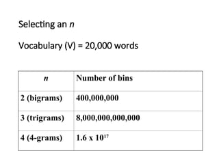
10. Selecting an n
Vocabulary (V) = 20,000 words
n Number of bins
2 (bigrams) 400,000,000
3 (trigrams) 8,000,000,000,000
4 (4-grams) 1.6 x 1017

11. 11

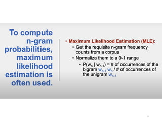
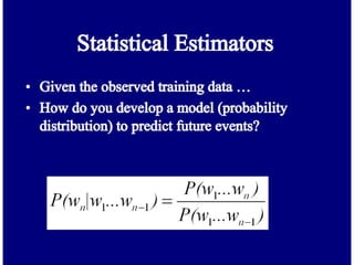
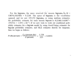
12. Statistical Estimators
• Given the observed training data …
• How do you develop a model (probability distribution) to predict
future events?

13. Statistical Estimators
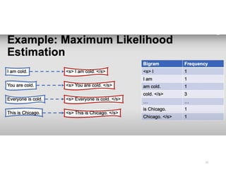
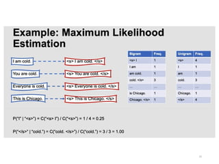
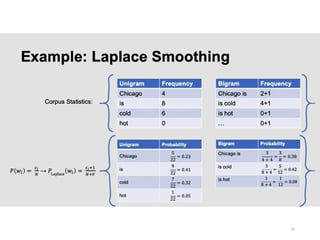
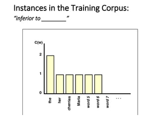
Example:
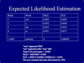
Corpus: five Jane Austen novels
N = 617,091 words
V = 14,585 unique words
Task: predict the next word of the trigram
“inferior to ________”
from test data, Persuasion: “[In person, she was]
inferior to both [sisters.]”

14. Building n-gram models
• Corpus- Jane Austen’s novels
• preprocess the corpus- removing all punctuation
14

15. Statistical Estimators I: Overview
•Goal: To derive a good probability estimate for the
target feature based on observed data
•Running Example: From n-gram data P(w1,..,wn)’s
predict P(wn|w1,..,wn-1)
•Solutions we will look at:
• Maximum Likelihood Estimation
• Laplace’s, Lidstone’s and Jeffreys-Perks’ Laws
• Held Out Estimation
• Cross-Validation
• Good-Turing Estimation
15

16. 16

17. 17

18. 18

19. 19

20. 20

21. 21

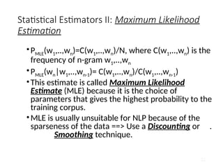
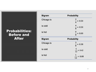
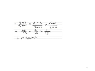
22. Statistical Estimators II: Maximum Likelihood
Estimation
•PMLE(w1,..,wn)=C(w1,..,wn)/N, where C(w1,..,wn) is the
frequency of n-gram w1,..,wn
•PMLE(wn|w1,..,wn-1)= C(w1,..,wn)/C(w1,..,wn-1)
•This estimate is called Maximum Likelihood
Estimate (MLE) because it is the choice of
parameters that gives the highest probability to the
training corpus.
•MLE is usually unsuitable for NLP because of the
sparseness of the data ==> Use a Discounting or .
Smoothing technique.
22

23. 23

24. 24

25. 25

26. Corpus
• Calculate probability of
• Chain rule:
26

27. Markov Assumption
• Compute probability of
• Wkt
• hence
27

28. • From the corpus we have
28

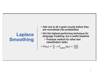
29. Statistical Estimators III: Smoothing
Techniques: Laplace
•PLAP(w1,..,wn)=(C(w1,..,wn)+1)/(N+B), where
C(w1,..,wn) is the frequency of n-gram w1,..,wn and B
is the number of bins training instances are divided
into. ==> Adding One Process
•The idea is to give a little bit of the probability space
to unseen events.
•However, in NLP applications that are very sparse,
Laplace’s Law actually gives far too much of the
probability space to unseen events.
29

30. 30

31. 31

32. 32

33. 33

34. 34

35. 35

36. 36

37. Example 2:
• The solution cannot be zero
37

38. Solution: Laplace Smoothing/ Add 1-
smoothing or Add n-smoothing
• Add 1-smoothing
• Add n-smoothing
• In our example:
38

39. 39

40. 40

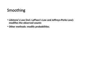
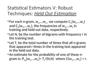
41. Statistical Estimators
Example:
Corpus: five Jane Austen novels
N = 617,091 words
V = 14,585 unique words
Task: predict the next word of the trigram “inferior
to ________”
from test data, Persuasion: “[In person, she was]
inferior to both [sisters.]”

42. Instances in the Training Corpus:
“inferior to ________”

43. Maximum Likelihood Estimate:

44. Actual Probability Distribution:

45. Actual Probability Distribution:

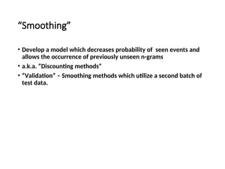
46. “Smoothing”
• Develop a model which decreases probability of seen events and
allows the occurrence of previously unseen n-grams
• a.k.a. “Discounting methods”
• “Validation” – Smoothing methods which utilize a second batch of
test data.

47. 47

48. 48

49. 49

50. Chapter 6:
Statistical Inference: n-gram
Models over Sparse Data

51. Statistical Estimators IV: Smoothing
Techniques:Lidstone and Jeffrey-Perks
•Since the adding one process may be adding too
much, we can add a smaller value .
•PLID(w1,..,wn)=(C(w1,..,wn)+)/(N+B), where
C(w1,..,wn) is the frequency of n-gram w1,..,wn and
B is the number of bins training instances are
divided into, and >0. ==> Lidstone’s Law
•If =1/2, Lidstone’s Law corresponds to the
expectation of the likelihood and is called the
Expected Likelihood Estimation (ELE) or the
Jeffreys-Perks Law.
51

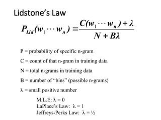
52. Lidstone’s Law
P = probability of specific n-gram
C = count of that n-gram in training data
N = total n-grams in training data
B = number of “bins” (possible n-grams)
 = small positive number
M.L.E:  = 0
LaPlace’s Law:  = 1
Jeffreys-Perks Law:  = ½
Bλ
N
λ
)
w
C(w
)
w
(w
P n
n
Lid




 1
1

53. Jeffreys-Perks Law

54. Objections to Lidstone’s Law
• Need an a priori way to determine .
• Predicts all unseen events to be equally likely
• Gives probability estimates linear in the M.L.E. frequency

55. 55

56. Smoothing
• Lidstone’s Law (incl. LaPlace’s Law and Jeffreys-Perks Law):
modifies the observed counts
• Other methods: modify probabilities.

57. Statistical Estimators V: Robust
Techniques: Held Out Estimation
•For each n-gram, w1,..,wn , we compute C1(w1,..,wn)
and C2(w1,..,wn), the frequencies of w1,..,wn in
training and held out data, respectively.
•Let Nr be the number of bigrams with frequency r in
the training text.
•Let Tr be the total number of times that all n-grams
that appeared r times in the training text appeared
in the held out data.
•An estimate for the probability of one of these n-
gram is: Pho(w1,..,wn)= Tr/(NrN) where C(w1,..,wn) = r.
57

58. Held-Out Estimator
• How much of the probability distribution should be “held out” to
allow for previously unseen events?
• Validate by holding out part of the training data.
• How often do events unseen in training data occur in validation
data?
(e.g., to choose  for Lidstone model)

59. 59

60. Testing Models
• Hold out ~ 5 – 10% for testing
• Hold out ~ 10% for validation (smoothing)
• For testing: useful to test on multiple sets of data, report variance
of results.
• Are results (good or bad) just the result of chance?

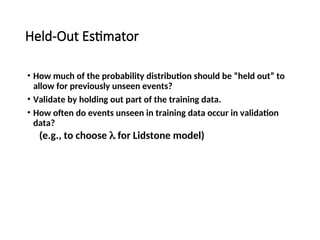
61. Statistical Estimators VI: Robust
Techniques: Cross-Validation
•Held Out estimation is useful if there is a lot of data
available. If not, it is useful to use each part of the
data both as training data and held out data.
•Deleted Estimation [Jelinek & Mercer, 1985]: Let
Nr
a
be the number of n-grams occurring r times in
the ath
part of the training data and Tr
ab
be the total
occurrences of those bigrams from part a in part b.
Pdel(w1,..,wn)= (Tr
01
+Tr
10
)/N(Nr
0
+Nr
1
) where
C(w1,..,wn) = r.
61

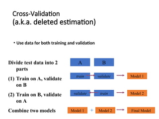
62. Cross-Validation
(a.k.a. deleted estimation)
• Use data for both training and validation
Divide test data into 2
parts
(1) Train on A, validate
on B
(2) Train on B, validate
on A
Combine two models
A B
train validate
validate train
Model 1
Model 2
Model 1 Model 2
+ Final Model

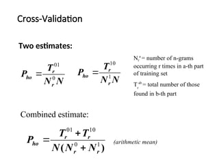
63. Cross-Validation
Two estimates:
Combined estimate:
Nr
a
= number of n-grams
occurring r times in a-th part
of training set
Tr
ab
= total number of those
found in b-th part
(arithmetic mean)
N
N
T
P
r
r
ho 0
01

N
N
T
P
r
r
ho 1
10

)
( 1
0
10
01
r
r
r
r
ho
N
N
N
T
T
P




64. Statistical Estimators VI: Related
Approach: Good-Turing Estimator
• Good (1953) attributes to Turing a method for
determining frequency or probability estimates of items,
on the assumption that their distribution is binomial.
• This method is suitable for large numbers of
observations of data drawn from a large vocabulary,
• and works well for n-grams, despite the fact that words
and n-grams do not have a binomial distribution.
64

65. 65

66. GTE with a uniform estimate for unseen
events
66

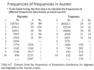
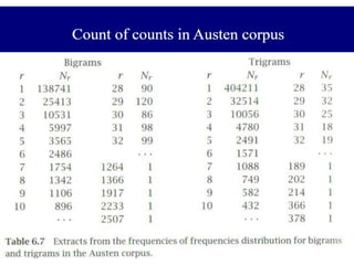
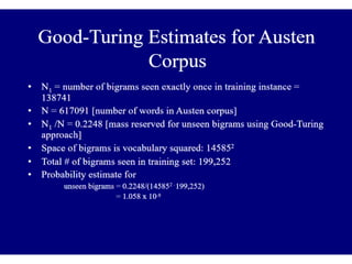
67. Frequencies of frequencies in Austen
• To do Good-Turing, the first step is to calculate the frequencies of
different frequencies (also known as count-counts).
67

68. 68
Table 6.9 Good-Turing bigram
frequency estimates for the
clause from Persuasion

69. 69

70. 70

71. 71

72. 72

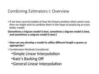
73. Combining Estimators I: Overview
• If we have several models of how the history predicts what comes next,
then we might wish to combine them in the hope of producing an even
better model.
(Sometimes a trigram model is best, sometimes a bigram model is best,
and sometimes a unigram model is best.)
• How can you develop a model to utilize different length n-grams as
appropriate?
• Combination Methods Considered:
•Simple Linear Interpolation
•Katz’s Backing Off
•General Linear Interpolation
73

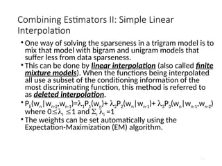
74. Combining Estimators II: Simple Linear
Interpolation
• One way of solving the sparseness in a trigram model is to
mix that model with bigram and unigram models that
suffer less from data sparseness.
• This can be done by linear interpolation (also called finite
mixture models). When the functions being interpolated
all use a subset of the conditioning information of the
most discriminating function, this method is referred to
as deleted interpolation.
• Pli(wn|wn-2,wn-1)=1P1(wn)+ 2P2(wn|wn-1)+ 3P3(wn|wn-1,wn-2)
where 0i 1 and i i =1
• The weights can be set automatically using the
Expectation-Maximization (EM) algorithm.
74

75. Simple Linear Interpolation
(a.k.a., finite mixture models;
a.k.a., deleted interpolation)
• weighted average of unigram, bigram, and trigram probabilities

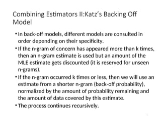
76. Combining Estimators II:Katz’s Backing Off
Model
• In back-off models, different models are consulted in
order depending on their specificity.
• If the n-gram of concern has appeared more than k times,
then an n-gram estimate is used but an amount of the
MLE estimate gets discounted (it is reserved for unseen
n-grams).
• If the n-gram occurred k times or less, then we will use an
estimate from a shorter n-gram (back-off probability),
normalized by the amount of probability remaining and
the amount of data covered by this estimate.
• The process continues recursively.
76

77. Katz’s Backing-Off
• Use n-gram probability when enough training data
• (when adjusted count > k; k usu. = 0 or 1)
• If not, “back-off” to the (n-1)-gram probability
• (Repeat as needed)

78. Problems with Backing-Off
• If bigram w1 w2 is common
• but trigram w1 w2 w3 is unseen
• may be a meaningful gap, rather than a gap due to chance and
scarce data
• i.e., a “grammatical null”
• May not want to back-off to lower-order probability

79. Combining Estimators II: General Linear
Interpolation
• In simple linear interpolation, the weights were just a single number, but one can define a
more general and powerful model where the weights are a function of the history.
• For k probability functions Pk, the general form for a linear interpolation model is:
• Linear interpolation is commonly used because it is a very general way to combine models.
• Randomly adding in dubious models to a linear interpolation need not do harm providing
one finds a good weighting of the models using the EM algorithm.
• But linear interpolation can make bad use of component models, especially if there is not a
careful partitioning of the histories with different weights used for different sorts of
histories.
79