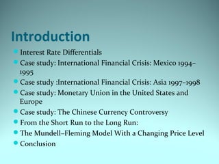
The document discusses several topics related to open economies and exchange rate regimes:
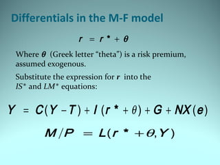
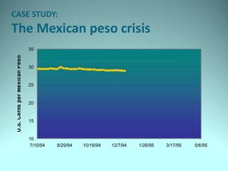
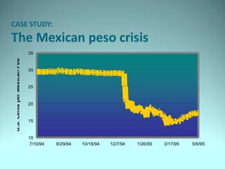
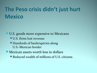
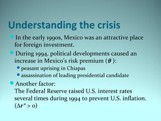
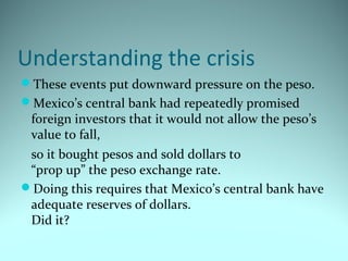
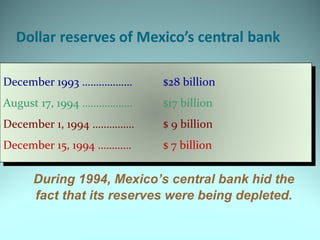
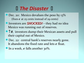
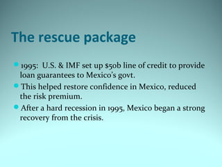
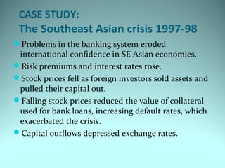
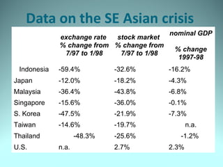
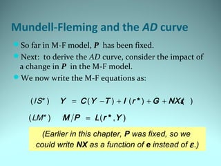
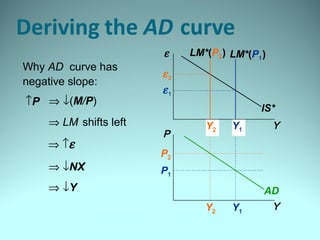
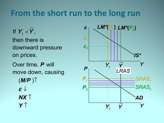
1) It examines the Mundell-Fleming model which models a small open economy using IS-LM curves with the exchange rate as an additional variable. Case studies on currency crises in Mexico and Asia are summarized.
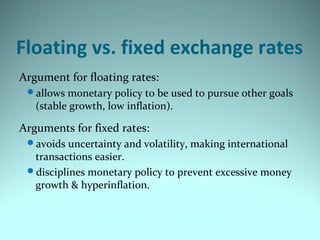
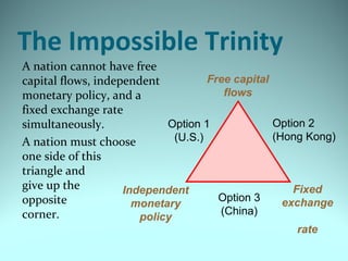
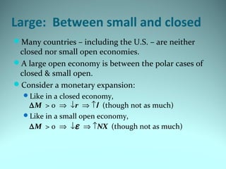
2) Issues related to floating vs fixed exchange rates and the impossible trinity are covered. Maintaining a fixed exchange rate limits independent monetary policy.
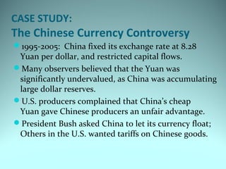
3) The Chinese currency controversy is discussed, noting China fixed its currency for years while accumulating dollar reserves, to the criticism of some arguing it was undervalued.