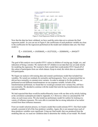
1) The document describes analyzing a dataset containing measurements from 654 youth to build a regression model for predicting forced expiratory volume (FEV1) based on age, height, sex, and smoking status.
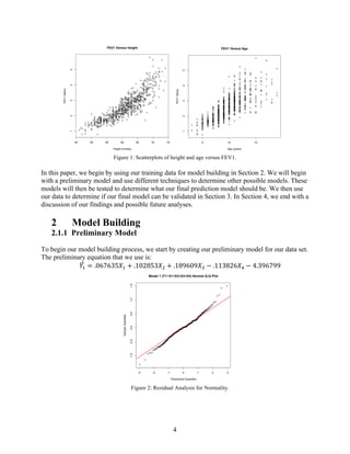
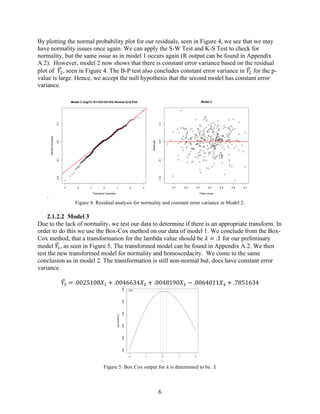
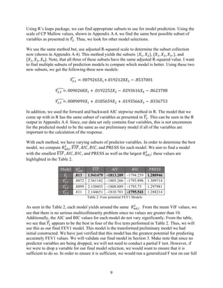
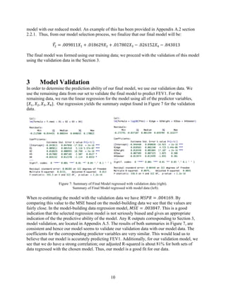
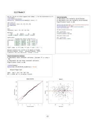
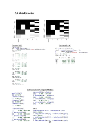
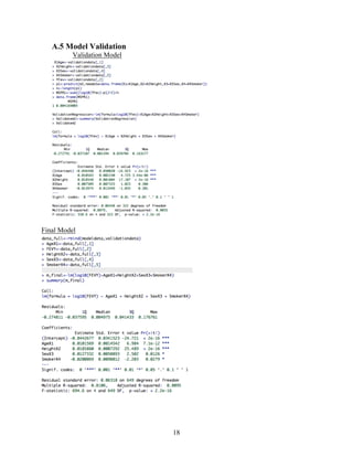
2) The preliminary model showed issues with non-normality and non-constant variance. Various transformations were tested, with the best being a log transformation of FEV1 (model 2).
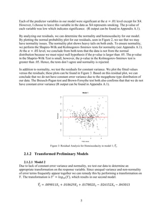
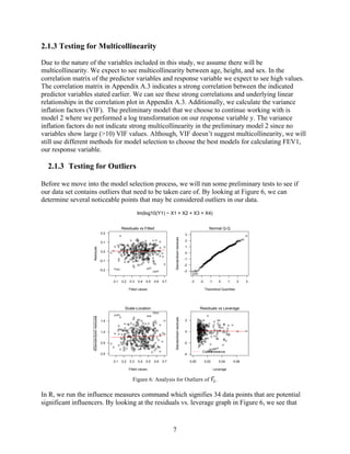
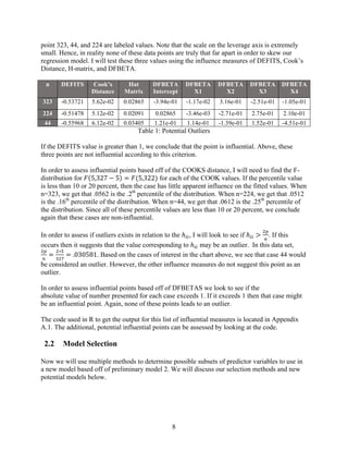
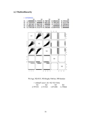
3) Tests for multicollinearity and outliers were also run, with some correlation between predictors but no significant outliers found that required removal from the dataset.
![1
Forced Expiratory Volume Regression Model
Katie Ruben
February 29, 2016
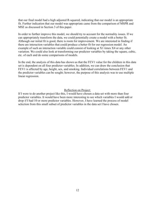
Forced expiratory volume (FEV1) is the volume of air forcibly expired in the first second of
maximal expiration after a maximal inspiration. FEV1 is a significant parameter for identifying
restrictive and obstructive respiratory diseases like asthma. It is a useful measure of how quickly
full lungs can be emptied. A common clinical technique to measure this quantity is through
Spirometry. Spirometry measures the rate at which the lung changes volume. The volume of the
capacity of a lung is measured in liters. Results received from a spirometry test are dependent on
the effort and cooperation between patients and examiners. These results depend heavily on the
technicality of implementation as well as personal attributes of the patient [2]. Personal attributes
that will help determine an accurate FEV1 score will be the patient's age, height, sex, and
indication of being a smoker or non-smoker.
The data used during this simulation comes from the Journal of Statistics Education Archive [3].
The data set consists of 4 variables, some of which are directly measured and some that are
qualitative in nature.
The data set is composed of a sample population consisting of 654 youth, male and female, aged
between 3 and 19 years old from the East Boston area in the late 1970’s [5]. This data set
contains 4 variables of measurement of children including age (years), height (inches), sex
(male/female), and their self indication about being a smoker (yes/no). An investigation of the
relationship between a child’s FEV1 and their current smoking status will be sought. It is
important to note that the younger the child, the lower their FEV1 lung capacity will be due to
the stature of their body alone. Therefore, in a normal case, the older the child is, the higher the
lung capacity as their body grows.
Another good measure of lung capacity is looking at the ratio between FEV1 and FVC. Forced
vital capacity (FVC) is the maximum total volume of air expired after a maximal deep breath in,
which takes 6 seconds to fully expire. A normal ratio value for a person without pulmonary
obstruction is between 80% and 120% [1]. A percentage lower than 80% is indicative of
obstructive lung functions. Since a predicted FVC value is not provided in the data set, one could
use known formulas to calculate this value for male and female children based off of their
personal attributes [4]. However, in using the data provided to calculate the predicted FVC value
will result in using the parameters for each child twice. Once in the predicted FVC formula and
once again when I perform a regression analysis. This would not be a good idea. Therefore, I will
exclude the the FEV1 to FVC ratio from my analysis, but it is good background information in
interpreting a person’s lung function.
In order to analyze this data, I will use our predictor variables to construct a linear regression
model for predicting FEV1 values. Upon initial fittings, I will analyze the model and look for
any initial predicting issues. Additionally, I will interpret the analysis of the data in order to](https://image.slidesharecdn.com/71d14937-92c6-4f82-8914-4b5492a9dbc4-161010132815/85/MultipleLinearRegressionPaper-1-320.jpg)
![1
Forced Expiratory Volume Regression Model
Katie Ruben
February 29, 2016
Forced expiratory volume (FEV1) is the volume of air forcibly expired in the first second of
maximal expiration after a maximal inspiration. FEV1 is a significant parameter for identifying
restrictive and obstructive respiratory diseases like asthma. It is a useful measure of how quickly
full lungs can be emptied. A common clinical technique to measure this quantity is through
Spirometry. Spirometry measures the rate at which the lung changes volume. The volume of the
capacity of a lung is measured in liters. Results received from a spirometry test are dependent on
the effort and cooperation between patients and examiners. These results depend heavily on the
technicality of implementation as well as personal attributes of the patient [2]. Personal attributes
that will help determine an accurate FEV1 score will be the patient's age, height, sex, and
indication of being a smoker or non-smoker.
The data used during this simulation comes from the Journal of Statistics Education Archive [3].
The data set consists of 4 variables, some of which are directly measured and some that are
qualitative in nature.
The data set is composed of a sample population consisting of 654 youth, male and female, aged
between 3 and 19 years old from the East Boston area in the late 1970’s [5]. This data set
contains 4 variables of measurement of children including age (years), height (inches), sex
(male/female), and their self indication about being a smoker (yes/no). An investigation of the
relationship between a child’s FEV1 and their current smoking status will be sought. It is
important to note that the younger the child, the lower their FEV1 lung capacity will be due to
the stature of their body alone. Therefore, in a normal case, the older the child is, the higher the
lung capacity as their body grows.
Another good measure of lung capacity is looking at the ratio between FEV1 and FVC. Forced
vital capacity (FVC) is the maximum total volume of air expired after a maximal deep breath in,
which takes 6 seconds to fully expire. A normal ratio value for a person without pulmonary
obstruction is between 80% and 120% [1]. A percentage lower than 80% is indicative of
obstructive lung functions. Since a predicted FVC value is not provided in the data set, one could
use known formulas to calculate this value for male and female children based off of their
personal attributes [4]. However, in using the data provided to calculate the predicted FVC value
will result in using the parameters for each child twice. Once in the predicted FVC formula and
once again when I perform a regression analysis. This would not be a good idea. Therefore, I will
exclude the the FEV1 to FVC ratio from my analysis, but it is good background information in
interpreting a person’s lung function.
In order to analyze this data, I will use our predictor variables to construct a linear regression
model for predicting FEV1 values. Upon initial fittings, I will analyze the model and look for
any initial predicting issues. Additionally, I will interpret the analysis of the data in order to](https://image.slidesharecdn.com/71d14937-92c6-4f82-8914-4b5492a9dbc4-161010132815/75/MultipleLinearRegressionPaper-1-2048.jpg)
![3
1 Background
Forced expiratory volume (FEV1) is the volume of air forcibly expired in the first second of
maximal expiration after a maximal inspiration. FEV1 is a significant parameter for identifying
restrictive and obstructive respiratory diseases like asthma. It is a useful measure of how quickly,
full lungs can be emptied. A common clinical technique to measure this quantity is through
Spirometry. Spirometry measures the rate at which the lung changes volume. The volume of the
capacity of a lung is measured in liters. Results received from a spirometry test are dependent on
the effort and cooperation between patients and examiners. These results depend heavily on the
technicality of implementation as well as personal attributes of the patient [2]. Personal attributes
that will help determine an accurate FEV1 score will be the patient's age, height, sex, and
indication of being a smoker or non-smoker.
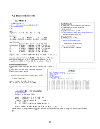
VARIABLE DESCRIPTION
𝒀 FEV1 (liters)
𝑿 𝟏 Age (years)
𝑿 𝟐 Height (inches)
𝑿 𝟑 Sex (male or female)
𝑿 𝟒 Smoker (yes or no)
Table 1: Variable Descriptions
For our model prediction analysis, we use a data set containing four variables. This data set is
from The Journal of Statistical Education and publically shared by Michael Kahn [3] with the
approval of Bernard Rosner who published the data in 1999 in Fundamentals of Biostatistics [5].
The data set is composed of a sample population consisting of 654 youth, male and female, aged
between 3 and 19 years old from the East Boston area in the late 1970’s. An investigation of the
relationship between a child’s FEV1 and their current smoking status will be sought as well as
any other comparisons between predictor variables. The variable descriptions can be found in
table 1. The indication of smoking for predictor variable 𝑋4, is qualitative data about each child.
The child made an indication if they, themselves were smokers or not while the data was being
collected.
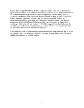
It is important to note that the younger the child, the lower their FEV1 lung capacity will be due
to the stature of their body alone. Therefore, in a normal case, the older the child is, the higher
the lung capacity as their body grows. As seen in Figure 1, the taller the child is then the higher
their FEV1. In addition, Figure 1 shows that in general as the child gets older their FEV1
increase however further investigation is needed into the interpretation of the FEV1 versus age
scatterplot. There may exist other factors that result in a drop of FEV1 as the children reach
puberty. We aim to find our best linear regression model for predicting FEV1 based off of our
four predictor variables; age, height, sex, and indication of smoking. In our model building
process we will want to determine if we can predict FEV1 using less measurements.](https://image.slidesharecdn.com/71d14937-92c6-4f82-8914-4b5492a9dbc4-161010132815/85/MultipleLinearRegressionPaper-3-320.jpg)
![13
Appendix
A Reference for Model Building
A.1 Preliminary Model
Model One: Y1~x1+x2+x3+x4:
s1
Call:
lm(formula = Y1 ~ X1 + X2 + X3 + X4)
Residuals:
Min 1Q Median 3Q Max
-1.31452 -0.22975 0.00576 0.24448 1.49585
Coefficients:
Estimate Std. Error t value Pr(>|t|)
(Intercept) -4.396799 0.310140 -14.177 < 2e-16 ***
X1 0.067625 0.012641 5.350 1.68e-07 ***
X2 0.102853 0.006546 15.713 < 2e-16 ***
X3 0.189609 0.046818 4.050 6.43e-05 ***
X4 -0.113826 0.081545 -1.396 0.164
---
Signif. codes: 0 ‘***’ 0.001 ‘**’ 0.01 ‘*’ 0.05 ‘.’ 0.1 ‘ ’ 1
Residual standard error: 0.4089 on 322 degrees of freedom
Multiple R-squared: 0.7784, Adjusted R-squared: 0.7756
F-statistic: 282.7 on 4 and 322 DF, p-value: < 2.2e-16
Tests
for
Normality:
𝐻@:Residuals are normally distributed.
𝐻Q:Residuals are not normally
distributed.
Significance level ∝=. 𝟎𝟓
>ks.test(residuals(m1),"pnorm", mean=0,
sd=sd(residuals(m1)))
KS-Test:
One-sample Kolmogorov-Smirnov test
data: residuals(m1)
D = 0.054421, p-value = 0.2875 >.05
alternative hypothesis: two-sided
>shapiro.test(residuals(m1))
Shapiro Test:
Shapiro-Wilk normality test
data: residuals(m1)
W = 0.9889, p-value = 0.01356 <.05
Tests
for
Constant
Error
Variance:
𝐻@:Residuals have constant variance. (accept if 𝑝 − 𝑣𝑎𝑙𝑢𝑒 >. 𝟎𝟓
𝐻Q:Residuals do not have constant variance.
Significance level ∝=. 𝟎𝟓
Brown Forsythe Test:
In order to split my data into two groups, I looked at the age of my participants. Group one contains 155
observations for their Age<=9 and group two contains 172 observations for their Age>=10.
library(car)
data.BF1<- modeldata[order(modeldata[,1]),]
X1.newBF1<-data.BF1[,1]
X2.newBF1<-data.BF1[,3]
X3.newBF1<-data.BF1[,4]
X4.newBF1<-data.BF1[,5]
Y.newBF1<-data.BF1[,2]
z.BF1<-residuals(lm(Y.newBF1~X1.newBF1+X2.newBF1+X3.newBF1+X4.newBF1))
g1<-rep(0,155)
g2<-rep(1,172)
group<-as.factor(c(g1,g2))
leveneTest(z.BF1,group)
Levene's Test for Homogeneity of Variance (center = median)
Df F value Pr(>F)
group 1 20.906 6.867e-06 ***
325
---
Signif. codes: 0 ‘***’ 0.001 ‘**’ 0.01 ‘*’ 0.05 ‘.’ 0.1 ‘ ’ 1
BP Test:
library(lmtest)
bptest(Y1~X1+X2+X3+X4,studentize = FALSE)
Breusch-Pagan test
data: Y1 ~ X1 + X2 + X3 + X4
BP = 48.145, df = 4, p-value = 8.803e-10](https://image.slidesharecdn.com/71d14937-92c6-4f82-8914-4b5492a9dbc4-161010132815/85/MultipleLinearRegressionPaper-13-320.jpg)
![19
References
[1] Barreiro, T. J., D.O., & Perillo, I., M.D. (2004, March). An Approach to Interpreting
Spirometry. Retrieved February 10, 2016, from http://www.aafp.org/afp/2004/0301/p1107.html
[2] Kavitha, A., Sujatha, C. M., & Ramakrishnan, S. (2010). Prediction of Spirometric Forced
Expiratory Volume (FEV1) Data Using Support Vector Regression. Measurement Science
Review, 10(2). Retrieved February 8, 2016, from
http://www.measurement.sk/2010/S1/Kavitha.pdf
[3] Michael, K. (2005). An Exhalent Problem for Teaching Statistics. Retrieved February 10,
2016, from http://www.amstat.org/publications/jse/v13n2/datasets.kahn.html
Journal of Statistics Education Volume 13, Number 2 (2005),
www.amstat.org/publications/jse/v13n2/datasets.kahn.html
[4] Knudson, RJ, et. al. The Maximal Expiratory Flow-Volume Curve Normal Standards,
Variability, and Effects of Age. Am. Rev. Respir. Dis. 113:589-590, 1976. Retrieved February 8,
2016, from http://cysticfibrosis.com/forums/topic/fev1/
[5] Rosner, B. (1999), Fundamentals of Biostatistics, 5th ed., Pacific Grove, CA: Duxbury.](https://image.slidesharecdn.com/71d14937-92c6-4f82-8914-4b5492a9dbc4-161010132815/85/MultipleLinearRegressionPaper-19-320.jpg)


