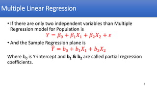
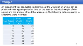
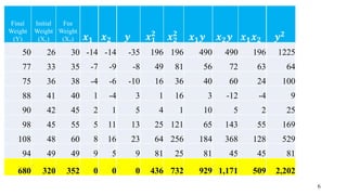
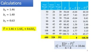
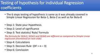
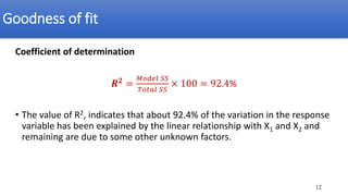
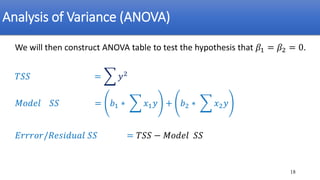
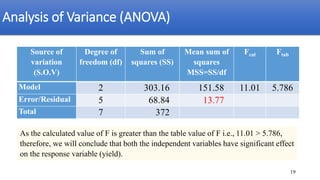
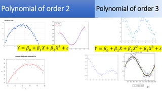
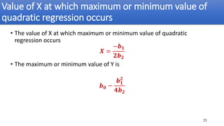
Multiple Linear Regression
&
Polynomial Regression
1
Multiple Linear Regression
• Multiple linear regression is a relationship that describes the
dependence of mean value of the response variable (Y) for given
values of two or more independent variables (X’s).
• Yield of a crop depends upon the fertility of the land, dose of the
fertilizer applied, quantity of seed etc.
• The grade point average of students depend on aptitude, mental ability,
hours devoted to study, nature of grading by teachers.
• The systolic blood pressure of a person depends upon one’s weight, age
etc.
2
Multiple Linear Regression
• If there are only two independent variables than Multiple
Regression model for Population is
𝑌 = 𝛽0 + 𝛽1𝑋1 + 𝛽2𝑋2 + 𝜀
• And the Sample Regression plane is
෠
𝑌 = 𝑏0 + 𝑏1𝑋1 + 𝑏2𝑋2
Where b0 is Y-intercept and b1 & b2 are called partial regression
coefficients.
3
Estimation of Parameters
b0 is the mean value of Y when
X1 = X2 = 0
b2 measures the average change in Y
for unit increase in X2 when the effect
of X1 is held constant
b1 is average change (increase or
decrease) in response variable Y for a
unit increase in the explanatory
variable X1 when the effect of X2 is
held constant
4
𝑏1 =
σ 𝑥2
2
σ 𝑥1𝑦 − σ 𝑥1𝑥2 σ 𝑥2𝑦
σ 𝑥1
2
σ 𝑥2
2
− σ 𝑥1𝑥2
2
𝑏2 =
σ 𝑥1
2
σ 𝑥2𝑦 − σ 𝑥1𝑥2 σ 𝑥1𝑦
σ 𝑥1
2
σ 𝑥2
2
− σ 𝑥1𝑥2
2
𝑏0 = ത
𝑌 − 𝑏1
ത
𝑋1 − 𝑏2
ത
𝑋2
Example
5
An experiment was conducted to determine if the weight of an animal can be
predicted after a given period of time on the basis of the initial weight of the
animal and the amount of feed that was eaten. The following data, measured in
kilograms, were recorded:
Final Weight
(Y)
Initial
Weight
(X1)
Feed
Weight
(X2)
50 26 30
77 33 35
75 36 38
88 41 40
90 42 45
98 45 55
108 48 60
94 49 49
6
Final
Weight
(Y)
Initial
Weight
(X1)
Fee
Weight
(X2)
50 26 30
77 33 35
75 36 38
88 41 40
90 42 45
98 45 55
108 48 60
94 49 49
680 320 352
𝒙𝟐
-14
-9
-6
-4
1
11
16
5
0
𝒚
-35
-8
-10
3
5
13
23
9
0
𝒙𝟏
𝟐
196
49
16
1
4
25
64
81
436
𝒙𝟐
𝟐
196
81
36
16
1
121
256
25
732
𝒙𝟏𝒚
490
56
40
3
10
65
184
81
929
𝒙𝟐𝒚
490
72
60
-12
5
143
368
45
1,171
𝒙𝟏𝒙𝟐
196
63
24
-4
2
55
128
45
509
𝒚𝟐
1225
64
100
9
25
169
529
81
2,202
𝒙𝟏
-14
-7
-4
1
2
5
8
9
0
Calculations
7
𝑏1 = 1.40
𝑏2 = 0.63
𝑏0 = 1.46
𝑆𝑒
2
=
σ 𝑌 − ෠
𝑌
2
𝑛 − 𝑘
= 33.66
Final
Weight
(Y)
Initial
Weight
(X1)
Fee
Weight
(X2)
50 26 30
77 33 35
75 36 38
88 41 40
90 42 45
98 45 55
108 48 60
94 49 49
680 320 352
෠
𝑌
56.64
69.57
75.64
83.89
88.42
98.89
106.23
100.72
𝑌 − ෠
𝑌
-6.64
7.43
-0.64
4.11
1.58
-0.89
1.77
-6.72
0
𝑌 − ෠
𝑌
𝟐
44.10
55.27
0.41
16.91
2.48
0.80
3.15
45.17
168.30
෠
𝑌 = 1.46 + 1.4𝑋1 + 0.63𝑋2
Testing of hypothesis for individual Regression
coefficients
• The 6 steps testing of hypothesis is same as it was already covered in
Simple Linear Regression for Beta-1, Beta-2 as well as for Beta-0
• Step-1: State your Hypothesis
• Step-2: Level of significance
• Step-3: Test statistic/ Rule/ Formula
The formula for SE(b1), SE(b2) and SE(b0) are different as compared to Simple Linear
regression (mentioned on next slide)
• Step-4: Calculations
• Step-5: Decision Rule (DF = n – 3)
• Step-6: Conclusion
8
9
𝑆𝐸(𝑏1) = 𝑆𝑒
2
σ 𝑥2
2
σ 𝑥1
2
σ 𝑥2
2
− σ 𝑥1𝑥2
2
= 0.64
Step-3 of the testing of hypothesis
𝑆𝐸(𝑏2) = 𝑆𝑒
2
σ 𝑥1
2
σ 𝑥1
2
σ 𝑥2
2
− σ 𝑥1𝑥2
2
= 0.49
Testing hypothesis
about 𝛽1
Testing hypothesis
about 𝛽2
𝑡 =
𝑏1 − 𝛽1
𝑆𝐸 𝑏1
𝑡 =
𝑏2 − 𝛽2
𝑆𝐸 𝑏2
Analysis of Variance (ANOVA)
We will then construct ANOVA table to test the hypothesis that 𝛽1 = 𝛽2 = 0.
𝑇𝑆𝑆 = ෍ 𝑦2
𝑀𝑜𝑑𝑒𝑙 𝑆𝑆 = 𝑏1 ∗ ෍ 𝑥1𝑦 + 𝑏2 ∗ ෍ 𝑥2𝑦
𝐸𝑟𝑟𝑟𝑜𝑟/𝑅𝑒𝑠𝑖𝑑𝑢𝑎𝑙 𝑆𝑆 = 𝑇𝑆𝑆 − 𝑀𝑜𝑑𝑒𝑙 𝑆𝑆
10
Analysis of Variance (ANOVA)
Source of
variation
(S.O.V)
Degree of
freedom (df)
Sum of
squares (SS)
Mean sum of
squares
MSS=SS/df
Fcal Ftab
Model 2 2033.7 1016.9 30.2 5.786
Error/Residual 5 168.3 33.7
Total 7 2202
As the calculated value of F is greater than the table value of F i.e., 30.2 > 5.786,
therefore, we will conclude that the model is significant.
11
Goodness of fit
Coefficient of determination
𝑹𝟐
=
𝑀𝑜𝑑𝑒𝑙 𝑆𝑆
𝑇𝑜𝑡𝑎𝑙 𝑆𝑆
× 100 = 92.4%
• The value of R2, indicates that about 92.4% of the variation in the response
variable has been explained by the linear relationship with X1 and X2 and
remaining are due to some other unknown factors.
12
Example
13
Computation of Multiple Linear Regression equation relating to Plant Height (X1) and
Tiller no. (X2) to Yield (Y) over 8 rice varieties
Grain yield
00 kg/hec
(Y)
Plant
Height cm
(X1)
Tiller no. /
hill (X2)
58 111 16
59 105 17
60 118 15
65 105 18
67 94 15
69 81 17
70 78 18
80 76 20
14
Grain
yield
00 kg/hec
(Y)
Plant
Height
cm (X1)
Tiller
no. / hill
(X2)
58 111 16
59 105 17
60 118 15
65 105 18
67 94 15
69 81 17
70 78 18
80 76 20
528 768 136
𝒙𝟐
-1
0
-2
1
-2
0
1
3
0
𝒚
-8
-7
-6
-1
1
3
4
14
0
𝒙𝟏
𝟐
225
81
484
81
4
225
324
400
1,824
𝒙𝟐
𝟐
1
0
4
1
4
0
1
9
20
𝒙𝟏𝒚
-120
-63
-132
-9
-2
-45
-72
-280
-723
𝒙𝟐𝒚
8
0
12
-1
-2
0
4
42
63
𝒙𝟏𝒙𝟐
-15
0
-44
9
4
0
-18
-60
-124
𝒚𝟐
64
49
36
1
1
9
16
196
372
𝒙𝟏
15
9
22
9
-2
-15
-18
-20
0
Calculations
15
𝑏1 = −0.32
𝑏2 = 1.2
𝑏0 = 75.89
𝑆𝑒
2
=
σ 𝑌 − ෠
𝑌
2
𝑛 − 3
= 13.77
Grain
yield
00 kg/hec
(Y)
Plant
Height
cm (X1)
Tiller
no. / hill
(X2)
58 111 16
59 105 17
60 118 15
65 105 18
67 94 15
69 81 17
70 78 18
80 76 20
528 768 136
෠
𝑌
60.08
63.16
56.68
64.36
64.24
70.73
72.87
75.89
𝑌 − ෠
𝑌
-2.08
-4.16
3.32
0.64
2.76
-1.73
-2.87
4.11
0.00
𝑌 − ෠
𝑌
𝟐
-2.08
-4.16
3.32
0.64
2.76
-1.73
-2.87
4.11
68.84
෠
𝑌 = 75.89 − 0.32𝑋1 + 1.2𝑋2
Testing of hypothesis for individual Regression
coefficients
• The 6 steps testing of hypothesis is same as it was already covered in
Simple Linear Regression for Beta-1, Beta-2 as well as for Beta-0
• Step-1: State your Hypothesis
• Step-2: Level of significance
• Step-3: Test statistic/ Rule/ Formula
The formula for SE(b1), SE(b2) and SE(b0) are different as compared to Simple Linear
regression (mentioned on next slide)
• Step-4: Calculations
• Step-5: Decision Rule (DF = n – 3)
• Step-6: Conclusion
16
17
𝑆𝐸(𝑏1) = 𝑆𝑒
2
σ 𝑥2
2
σ 𝑥1
2
σ 𝑥2
2
− σ 𝑥1𝑥2
2
= 0.11
Step-3 formulas of testing of hypothesis
𝑆𝐸(𝑏2) = 𝑆𝑒
2
σ 𝑥1
2
σ 𝑥1
2
σ 𝑥2
2
− σ 𝑥1𝑥2
2
= 1.09
Testing hypothesis
about 𝛽1
Testing hypothesis
about 𝛽2
𝑡 =
𝑏1 − 𝛽1
𝑆𝐸 𝑏1
𝑡 =
𝑏2 − 𝛽2
𝑆𝐸 𝑏2
Analysis of Variance (ANOVA)
We will then construct ANOVA table to test the hypothesis that 𝛽1 = 𝛽2 = 0.
𝑇𝑆𝑆 = ෍ 𝑦2
𝑀𝑜𝑑𝑒𝑙 𝑆𝑆 = 𝑏1 ∗ ෍ 𝑥1𝑦 + 𝑏2 ∗ ෍ 𝑥2𝑦
𝐸𝑟𝑟𝑟𝑜𝑟/𝑅𝑒𝑠𝑖𝑑𝑢𝑎𝑙 𝑆𝑆 = 𝑇𝑆𝑆 − 𝑀𝑜𝑑𝑒𝑙 𝑆𝑆
18
Analysis of Variance (ANOVA)
Source of
variation
(S.O.V)
Degree of
freedom (df)
Sum of
squares (SS)
Mean sum of
squares
MSS=SS/df
Fcal Ftab
Model 2 303.16 151.58 11.01 5.786
Error/Residual 5 68.84 13.77
Total 7 372
As the calculated value of F is greater than the table value of F i.e., 11.01 > 5.786,
therefore, we will conclude that both the independent variables have significant effect
on the response variable (yield).
19
Goodness of fit
Coefficient of determination
𝑹𝟐
=
𝐸𝑥𝑝𝑙𝑎𝑖𝑛𝑒𝑑 𝑣𝑎𝑟𝑖𝑎𝑡𝑖𝑜𝑛
𝑇𝑜𝑡𝑎𝑙 𝑣𝑎𝑟𝑖𝑎𝑡𝑖𝑜𝑛
× 100 = 81.5%
• The value of R2, indicates that about 81.5% of the variation in the response
variable has been explained by the linear relationship with X1 and X2 and
remaining are due to some other unknown factors.
20
Polynomial of order 2 Polynomial of order 3
21
Polynomial Regression
• Polynomial regression is a form of linear regression in which the
relationship between the independent variable X and the dependent
variable Y is modelled as an nth degree polynomial.
• The polynomial of order 2 is
• The polynomial of order 3 is
The estimation of Betas i.e., b0, b1, b2 is similar to the Multiple Regression.
22
Example
• Fit an appropriate regression model to describe the relationship b/w yield
response of rice variety and nitrogen fertilizer
Y
178
806
1383
1661
1591
1176
778
23
X
0
5
25
50
70
90
110
Example
24
X2
0
25
625
2500
4900
8100
12100
Y
178
806
1383
1661
1591
1176
778
X1
0
5
25
50
70
90
110
Value of X at which maximum or minimum value of
quadratic regression occurs
• The value of X at which maximum or minimum value of quadratic
regression occurs
𝑿 =
−𝒃𝟏
𝟐𝒃𝟐
• The maximum or minimum value of Y is
𝒃𝟎 −
𝒃𝟏
𝟐
𝟒𝒃𝟐
25
Thanks
26

Multiple and Polynomial Regression analysis with practical example

  • 1.
  • 2.
    Multiple Linear Regression •Multiple linear regression is a relationship that describes the dependence of mean value of the response variable (Y) for given values of two or more independent variables (X’s). • Yield of a crop depends upon the fertility of the land, dose of the fertilizer applied, quantity of seed etc. • The grade point average of students depend on aptitude, mental ability, hours devoted to study, nature of grading by teachers. • The systolic blood pressure of a person depends upon one’s weight, age etc. 2
  • 3.
    Multiple Linear Regression •If there are only two independent variables than Multiple Regression model for Population is 𝑌 = 𝛽0 + 𝛽1𝑋1 + 𝛽2𝑋2 + 𝜀 • And the Sample Regression plane is ෠ 𝑌 = 𝑏0 + 𝑏1𝑋1 + 𝑏2𝑋2 Where b0 is Y-intercept and b1 & b2 are called partial regression coefficients. 3
  • 4.
    Estimation of Parameters b0is the mean value of Y when X1 = X2 = 0 b2 measures the average change in Y for unit increase in X2 when the effect of X1 is held constant b1 is average change (increase or decrease) in response variable Y for a unit increase in the explanatory variable X1 when the effect of X2 is held constant 4 𝑏1 = σ 𝑥2 2 σ 𝑥1𝑦 − σ 𝑥1𝑥2 σ 𝑥2𝑦 σ 𝑥1 2 σ 𝑥2 2 − σ 𝑥1𝑥2 2 𝑏2 = σ 𝑥1 2 σ 𝑥2𝑦 − σ 𝑥1𝑥2 σ 𝑥1𝑦 σ 𝑥1 2 σ 𝑥2 2 − σ 𝑥1𝑥2 2 𝑏0 = ത 𝑌 − 𝑏1 ത 𝑋1 − 𝑏2 ത 𝑋2
  • 5.
    Example 5 An experiment wasconducted to determine if the weight of an animal can be predicted after a given period of time on the basis of the initial weight of the animal and the amount of feed that was eaten. The following data, measured in kilograms, were recorded: Final Weight (Y) Initial Weight (X1) Feed Weight (X2) 50 26 30 77 33 35 75 36 38 88 41 40 90 42 45 98 45 55 108 48 60 94 49 49
  • 6.
    6 Final Weight (Y) Initial Weight (X1) Fee Weight (X2) 50 26 30 7733 35 75 36 38 88 41 40 90 42 45 98 45 55 108 48 60 94 49 49 680 320 352 𝒙𝟐 -14 -9 -6 -4 1 11 16 5 0 𝒚 -35 -8 -10 3 5 13 23 9 0 𝒙𝟏 𝟐 196 49 16 1 4 25 64 81 436 𝒙𝟐 𝟐 196 81 36 16 1 121 256 25 732 𝒙𝟏𝒚 490 56 40 3 10 65 184 81 929 𝒙𝟐𝒚 490 72 60 -12 5 143 368 45 1,171 𝒙𝟏𝒙𝟐 196 63 24 -4 2 55 128 45 509 𝒚𝟐 1225 64 100 9 25 169 529 81 2,202 𝒙𝟏 -14 -7 -4 1 2 5 8 9 0
  • 7.
    Calculations 7 𝑏1 = 1.40 𝑏2= 0.63 𝑏0 = 1.46 𝑆𝑒 2 = σ 𝑌 − ෠ 𝑌 2 𝑛 − 𝑘 = 33.66 Final Weight (Y) Initial Weight (X1) Fee Weight (X2) 50 26 30 77 33 35 75 36 38 88 41 40 90 42 45 98 45 55 108 48 60 94 49 49 680 320 352 ෠ 𝑌 56.64 69.57 75.64 83.89 88.42 98.89 106.23 100.72 𝑌 − ෠ 𝑌 -6.64 7.43 -0.64 4.11 1.58 -0.89 1.77 -6.72 0 𝑌 − ෠ 𝑌 𝟐 44.10 55.27 0.41 16.91 2.48 0.80 3.15 45.17 168.30 ෠ 𝑌 = 1.46 + 1.4𝑋1 + 0.63𝑋2
  • 8.
    Testing of hypothesisfor individual Regression coefficients • The 6 steps testing of hypothesis is same as it was already covered in Simple Linear Regression for Beta-1, Beta-2 as well as for Beta-0 • Step-1: State your Hypothesis • Step-2: Level of significance • Step-3: Test statistic/ Rule/ Formula The formula for SE(b1), SE(b2) and SE(b0) are different as compared to Simple Linear regression (mentioned on next slide) • Step-4: Calculations • Step-5: Decision Rule (DF = n – 3) • Step-6: Conclusion 8
  • 9.
    9 𝑆𝐸(𝑏1) = 𝑆𝑒 2 σ𝑥2 2 σ 𝑥1 2 σ 𝑥2 2 − σ 𝑥1𝑥2 2 = 0.64 Step-3 of the testing of hypothesis 𝑆𝐸(𝑏2) = 𝑆𝑒 2 σ 𝑥1 2 σ 𝑥1 2 σ 𝑥2 2 − σ 𝑥1𝑥2 2 = 0.49 Testing hypothesis about 𝛽1 Testing hypothesis about 𝛽2 𝑡 = 𝑏1 − 𝛽1 𝑆𝐸 𝑏1 𝑡 = 𝑏2 − 𝛽2 𝑆𝐸 𝑏2
  • 10.
    Analysis of Variance(ANOVA) We will then construct ANOVA table to test the hypothesis that 𝛽1 = 𝛽2 = 0. 𝑇𝑆𝑆 = ෍ 𝑦2 𝑀𝑜𝑑𝑒𝑙 𝑆𝑆 = 𝑏1 ∗ ෍ 𝑥1𝑦 + 𝑏2 ∗ ෍ 𝑥2𝑦 𝐸𝑟𝑟𝑟𝑜𝑟/𝑅𝑒𝑠𝑖𝑑𝑢𝑎𝑙 𝑆𝑆 = 𝑇𝑆𝑆 − 𝑀𝑜𝑑𝑒𝑙 𝑆𝑆 10
  • 11.
    Analysis of Variance(ANOVA) Source of variation (S.O.V) Degree of freedom (df) Sum of squares (SS) Mean sum of squares MSS=SS/df Fcal Ftab Model 2 2033.7 1016.9 30.2 5.786 Error/Residual 5 168.3 33.7 Total 7 2202 As the calculated value of F is greater than the table value of F i.e., 30.2 > 5.786, therefore, we will conclude that the model is significant. 11
  • 12.
    Goodness of fit Coefficientof determination 𝑹𝟐 = 𝑀𝑜𝑑𝑒𝑙 𝑆𝑆 𝑇𝑜𝑡𝑎𝑙 𝑆𝑆 × 100 = 92.4% • The value of R2, indicates that about 92.4% of the variation in the response variable has been explained by the linear relationship with X1 and X2 and remaining are due to some other unknown factors. 12
  • 13.
    Example 13 Computation of MultipleLinear Regression equation relating to Plant Height (X1) and Tiller no. (X2) to Yield (Y) over 8 rice varieties Grain yield 00 kg/hec (Y) Plant Height cm (X1) Tiller no. / hill (X2) 58 111 16 59 105 17 60 118 15 65 105 18 67 94 15 69 81 17 70 78 18 80 76 20
  • 14.
    14 Grain yield 00 kg/hec (Y) Plant Height cm (X1) Tiller no./ hill (X2) 58 111 16 59 105 17 60 118 15 65 105 18 67 94 15 69 81 17 70 78 18 80 76 20 528 768 136 𝒙𝟐 -1 0 -2 1 -2 0 1 3 0 𝒚 -8 -7 -6 -1 1 3 4 14 0 𝒙𝟏 𝟐 225 81 484 81 4 225 324 400 1,824 𝒙𝟐 𝟐 1 0 4 1 4 0 1 9 20 𝒙𝟏𝒚 -120 -63 -132 -9 -2 -45 -72 -280 -723 𝒙𝟐𝒚 8 0 12 -1 -2 0 4 42 63 𝒙𝟏𝒙𝟐 -15 0 -44 9 4 0 -18 -60 -124 𝒚𝟐 64 49 36 1 1 9 16 196 372 𝒙𝟏 15 9 22 9 -2 -15 -18 -20 0
  • 15.
    Calculations 15 𝑏1 = −0.32 𝑏2= 1.2 𝑏0 = 75.89 𝑆𝑒 2 = σ 𝑌 − ෠ 𝑌 2 𝑛 − 3 = 13.77 Grain yield 00 kg/hec (Y) Plant Height cm (X1) Tiller no. / hill (X2) 58 111 16 59 105 17 60 118 15 65 105 18 67 94 15 69 81 17 70 78 18 80 76 20 528 768 136 ෠ 𝑌 60.08 63.16 56.68 64.36 64.24 70.73 72.87 75.89 𝑌 − ෠ 𝑌 -2.08 -4.16 3.32 0.64 2.76 -1.73 -2.87 4.11 0.00 𝑌 − ෠ 𝑌 𝟐 -2.08 -4.16 3.32 0.64 2.76 -1.73 -2.87 4.11 68.84 ෠ 𝑌 = 75.89 − 0.32𝑋1 + 1.2𝑋2
  • 16.
    Testing of hypothesisfor individual Regression coefficients • The 6 steps testing of hypothesis is same as it was already covered in Simple Linear Regression for Beta-1, Beta-2 as well as for Beta-0 • Step-1: State your Hypothesis • Step-2: Level of significance • Step-3: Test statistic/ Rule/ Formula The formula for SE(b1), SE(b2) and SE(b0) are different as compared to Simple Linear regression (mentioned on next slide) • Step-4: Calculations • Step-5: Decision Rule (DF = n – 3) • Step-6: Conclusion 16
  • 17.
    17 𝑆𝐸(𝑏1) = 𝑆𝑒 2 σ𝑥2 2 σ 𝑥1 2 σ 𝑥2 2 − σ 𝑥1𝑥2 2 = 0.11 Step-3 formulas of testing of hypothesis 𝑆𝐸(𝑏2) = 𝑆𝑒 2 σ 𝑥1 2 σ 𝑥1 2 σ 𝑥2 2 − σ 𝑥1𝑥2 2 = 1.09 Testing hypothesis about 𝛽1 Testing hypothesis about 𝛽2 𝑡 = 𝑏1 − 𝛽1 𝑆𝐸 𝑏1 𝑡 = 𝑏2 − 𝛽2 𝑆𝐸 𝑏2
  • 18.
    Analysis of Variance(ANOVA) We will then construct ANOVA table to test the hypothesis that 𝛽1 = 𝛽2 = 0. 𝑇𝑆𝑆 = ෍ 𝑦2 𝑀𝑜𝑑𝑒𝑙 𝑆𝑆 = 𝑏1 ∗ ෍ 𝑥1𝑦 + 𝑏2 ∗ ෍ 𝑥2𝑦 𝐸𝑟𝑟𝑟𝑜𝑟/𝑅𝑒𝑠𝑖𝑑𝑢𝑎𝑙 𝑆𝑆 = 𝑇𝑆𝑆 − 𝑀𝑜𝑑𝑒𝑙 𝑆𝑆 18
  • 19.
    Analysis of Variance(ANOVA) Source of variation (S.O.V) Degree of freedom (df) Sum of squares (SS) Mean sum of squares MSS=SS/df Fcal Ftab Model 2 303.16 151.58 11.01 5.786 Error/Residual 5 68.84 13.77 Total 7 372 As the calculated value of F is greater than the table value of F i.e., 11.01 > 5.786, therefore, we will conclude that both the independent variables have significant effect on the response variable (yield). 19
  • 20.
    Goodness of fit Coefficientof determination 𝑹𝟐 = 𝐸𝑥𝑝𝑙𝑎𝑖𝑛𝑒𝑑 𝑣𝑎𝑟𝑖𝑎𝑡𝑖𝑜𝑛 𝑇𝑜𝑡𝑎𝑙 𝑣𝑎𝑟𝑖𝑎𝑡𝑖𝑜𝑛 × 100 = 81.5% • The value of R2, indicates that about 81.5% of the variation in the response variable has been explained by the linear relationship with X1 and X2 and remaining are due to some other unknown factors. 20
  • 21.
    Polynomial of order2 Polynomial of order 3 21
  • 22.
    Polynomial Regression • Polynomialregression is a form of linear regression in which the relationship between the independent variable X and the dependent variable Y is modelled as an nth degree polynomial. • The polynomial of order 2 is • The polynomial of order 3 is The estimation of Betas i.e., b0, b1, b2 is similar to the Multiple Regression. 22
  • 23.
    Example • Fit anappropriate regression model to describe the relationship b/w yield response of rice variety and nitrogen fertilizer Y 178 806 1383 1661 1591 1176 778 23 X 0 5 25 50 70 90 110
  • 24.
  • 25.
    Value of Xat which maximum or minimum value of quadratic regression occurs • The value of X at which maximum or minimum value of quadratic regression occurs 𝑿 = −𝒃𝟏 𝟐𝒃𝟐 • The maximum or minimum value of Y is 𝒃𝟎 − 𝒃𝟏 𝟐 𝟒𝒃𝟐 25
  • 26.