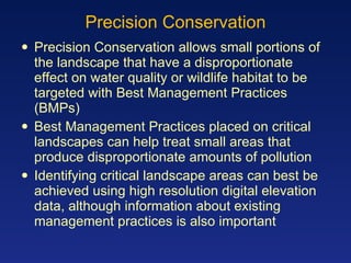
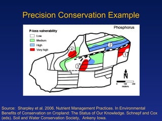
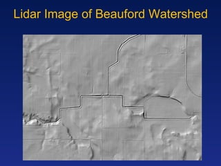
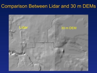
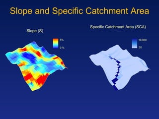
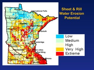
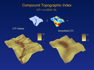
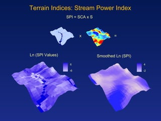
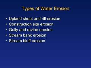
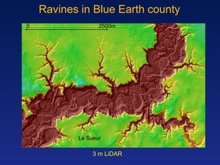
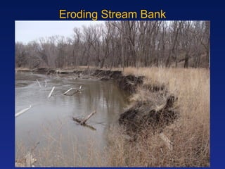
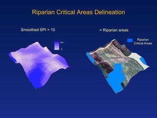
The document discusses the need for high resolution digital elevation data to identify critical areas for targeting conservation practices in Minnesota. Precision conservation, which focuses practices on disproportionately polluting areas, can better protect water quality and habitat than spreading practices evenly. Lidar data can help identify critical sources of runoff and pollution like upland depressions, eroding stream banks, and ravines. Targeting best management practices to these critical areas identified through terrain analysis of high resolution elevation data can maximize the impact of conservation efforts.

1. The Need for High Resolution Digital Elevation Data for Precision Conservation in Minnesota Dr. David Mulla Professor and W.E. Larson Chair for Soil and Water Resources Department of Soil, Water, & Climate University of Minnesota

2. Precision Conservation Precision Conservation allows small portions of the landscape that have a disproportionate effect on water quality or wildlife habitat to be targeted with Best Management Practices (BMPs) Best Management Practices placed on critical landscapes can help treat small areas that produce disproportionate amounts of pollution Identifying critical landscape areas can best be achieved using high resolution digital elevation data, although information about existing management practices is also important

3. Precision Conservation (compared to Precision Ag) (From Berry, 2008 )

4. Precision Conservation Example Source: Sharpley et al. 2006. Nutrient Management Practices. In Environmental Benefits of Conservation on Cropland: The Status of Our Knowledge. Schnepf and Cox (eds). Soil and Water Conservation Society, Ankeny Iowa.

6. Precision Conservation Example Sites of Biodiversity Significance Wildlife Management Areas 250m buffer around current WMAs and Biodiversity Sites

7. Clean Water Funding Initiatives Passage of the Clean Water Legacy Amendment provides badly needed funding for protection, restoration and enhancement of impaired waters and damaged wildlife habitat Funding from the Clean Water Legacy Amendment should be spent on the most critical landscapes and sources of degradation rather than spread evenly across the state There is a pressing need to identify critical sources of water quality degradation and their locations in order to select and implement BMPs

8. The 2008 Impaired Waters list contains 1,469 impairments including: 500 lakes 25 listed for multiple pollutants 336 rivers & streams 603 “reaches” w/many pollutants

9. Lake Pepin Watershed TMDL Sediment Phosphorus

10. Existing BMP Programs RIM program involved 203,000 acres enrolled in 5,300 conservation easements Program is heavily focused on Minnesota River Basin riparian areas and wetlands

11. Wildlife Management Areas (FY ‘07 & FY ‘08) Prairie Grassland Habitat 63,000 ac Wetland Habitat 201,000 ac Forest Habitat 32,000 ac

12. Conservation Reserve Program Enrolled Acreage Expiration Patterns

13. Variable Source Areas The variable source area concept explains how small portions of the landscape, termed critical source areas, can contribute disproportionately to runoff and peak flows during storm events (Brooks et al., 2003) Q TIME Q TIME T2 T1 *Modified from Brooks et al., 2003 & references

14. Critical Source Areas Critical source areas can include upland depressions, riparian areas, open culverts and tile outlets, gullies, ravines, eroding stream banks and slumping stream bluffs

15. Critical Area Problem Studies suggest that small areas of the agricultural landscape (5-25%) generate a disproportionately large amount of erosion or phosphorus The reduction of nonpoint source pollution loads at the outlet of agricultural watersheds is dependent on the implementation of best management practices (BMPs) in critical source areas of nonpoint source pollution Defining critical source areas is a challenge, but terrain analysis of digital elevation models (DEMs) is promising

16. Converging/Diverging Flows

17. Lidar Image of Beauford Watershed

18. Comparison Between Lidar and 30 m DEMs Lidar 30 m DEM

19. Terrain Attributes for Precision Conservation Terrain attributes can be derived from DEMs using… ESRI’s AcrGIS v. 9.2 TAUDEM v. 3.1 (Tarboton, 2005) D∞ method of flow routing (Tarboten, 1997) Critical source area data layers can be created by combining… Different thresholds applied to terrain attributes Ancillary GIS data (Soils drainage, Landuse/Landcover)

20. Slope (S) Specific Catchment Area (SCA) Slope and Specific Catchment Area 5% 0 % 30 10,000

21. Landscape slope Affects overland flow and erosion potential

22. Sheet & Rill Water Erosion Potential Duluth Bemidji Cambridge Twin cities Grand Forks Winona Rochester Pipestone Marshall Montevideo St. Cloud Roseau Moorhead Austin Mankato Morris Grand Rapids International Falls Ortonville Red Wing

23. CTI Values Smoothed CTI Compound Topographic Index 7 20 8 14 CTI = Ln (SCA / S) =

24. Characterizes soil water content and surface saturation zones Compound Topographic Index CTI = ln(As/tan S) As is specific catchment S is slope

25. Terrain Indices: Stream Power Index Ln (SPI Values) Smoothed Ln (SPI) -6 6 -2 4 SPI = SCA x S x =

26. Stream Power Index SPI = As tanS As is specific catchment area, S is slope Measures erosive power of overland flow

27. Types of Water Erosion Upland sheet and rill erosion Construction site erosion Gully and ravine erosion Stream bank erosion Stream bluff erosion

28. Deposition from Sheet & Rill Erosion

29. Construction Site Erosion

30. Ravine Erosion

31. Ravines in Blue Earth county 3 m LiDAR Le Sueur 0 2500m

32. Ravines in Blue Earth county 30 m DEM Le Sueur 0 2500m

33. Eroding Stream Bank

34. Stream Bluff Erosion

35. Disproportionalities The Le Sueur contributes a disproportionate amount of non-point source pollution to the Minnesota River Only comprises 7% of the basin land surface area 53% TSS 31% Total P 20% NO 3 -N (MRBDC, 2005) Data Source: ESRI & MN DNR Le Sueur River Watershed N Km 0 15 30 0 100 200 Km

36. Cobb River Slumping Bluff

37. Appendix D

38. Ravine Sediment Sources Digitized from Blue Earth county Lidar by Patrick Belmont - NCED

39. 8 14 Upland Depressions Delineation Smoothed CTI > 11.5 Drainage = “Poorly Drained” = Upland Depressions + Upland Depressions Critical Areas

40. Upland Depressions Covers nearly 20,000 ha (7%) in the Le Sueur Watershed 85% of upland depressions are in ag production Upland Depressions Critical Areas N Data source: MN DNR 0 20 40 Km

41. Upland Depressions Data source: MN DNR & MN LMIC N Upland Depressions Critical Areas 0 15 30 Km 0 2.5 5 Km 0 500 1,000 Meters

42. Riparian Critical Areas Delineation Smoothed SPI > 10 = Riparian areas 0 10+ Riparian Critical Areas

43. Critical Riparian Areas Riparian Critical Areas Covers over 25% of the watershed (~74,000ha) 59% of riparian critical areas are in ag production When combined with erosion potential, gives high priority areas needing BMPs N Data source: MN DNR 0 20 40 Km

44. Conclusions Disproportionate amounts of sediment and phosphorus are generated from small areas of the watershed The effectiveness of BMPs depends on placing them in vulnerable portions of the landscape Precision conservation strategies involving terrain analysis may prove very helpful in the future to guide conservation efforts tailored to specific landscapes and to maximize efficiency of their placement Lidar based DEMs can help improve the accuracy of identifying critical landscapes and targeting BMPs to critical areas

45. Thank You. Questions?