This document provides an overview of morphology in computational linguistics. It discusses topics like morphemes, inflectional versus derivational morphology, and morphological processes. It also describes how morphology is handled in natural language processing, including the use of finite state automata and transducers to model morphological rules and mappings between surface forms and underlying representations.
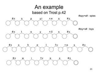
![Morphology
See
Harald Trost “Morphology”. Chapter 2 of R Mitkov (ed.) The
Oxford Handbook of Computational Linguistics, Oxford
(2004): OUP
D Jurafsky & JH Martin: Speech and Language Processing,
Upper Saddle River NJ (2000): Prentice Hall, Chapter 3
[quite technical]](https://image.slidesharecdn.com/morphology-220922141957-c059a204/85/Morphology-ppt-1-320.jpg)
![Morphology
See
Harald Trost “Morphology”. Chapter 2 of R Mitkov (ed.) The
Oxford Handbook of Computational Linguistics, Oxford
(2004): OUP
D Jurafsky & JH Martin: Speech and Language Processing,
Upper Saddle River NJ (2000): Prentice Hall, Chapter 3
[quite technical]](https://image.slidesharecdn.com/morphology-220922141957-c059a204/75/Morphology-ppt-1-2048.jpg)


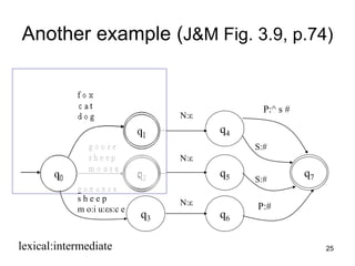
![27
q0
q6
q5
q4
q3
q2
q1
q7
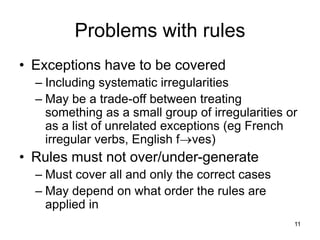
g o o s e
s h e e p
m o u s e
g o:e o:e s e
s h e e p
m o:i u:εs:c e
N:ε
N:ε
N:ε
P:^ s #
S:#
S:#
P:#
[0] f:f o:o x:x [1] N:ε [4] P:^ s:s #:# [7]
[0] f:f o:o x:x [1] N:ε [4] S:# [7]
[0] c:c a:a t:t [1] N:ε [4] P:^ s:s #:# [7]
[0] s:s h:h e:e p:p [2] N:ε [5] S:# [7]
[0] g:g o:e o:e s:s e:e [3] N:ε [5] P:# [7]
f o x N P s # : f o x ^ s #
f o x N S : f o x #
c a t N P s # : c a t ^ s #
s h e e p N S : s h e e p #
g o o s e N P : g e e s e #
f o x
c a t
d o g](https://image.slidesharecdn.com/morphology-220922141957-c059a204/85/Morphology-ppt-27-320.jpg)
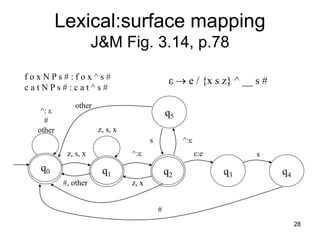
![29
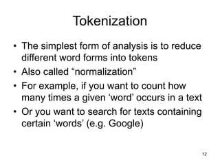
f o x ^ s # f o x e s #
c a t ^ s # : c a t ^ s #
q5
q4
q0 q2 q3
q1
^: ε
#
other
other
z, s, x
z, s, x
#, other z, x
^:ε
s ^:ε
ε:e s
#
[0] f:f [0] o:o [0] x:x [1] ^:ε [2] ε:e [3] s:s [4] #:# [0]
[0] c:c [0] a:a [0] t:t [0] ^:ε [0] s:s [0] #:# [0]](https://image.slidesharecdn.com/morphology-220922141957-c059a204/85/Morphology-ppt-29-320.jpg)
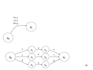
![31
FST compiler
http://www.xrce.xerox.com/competencies/content-analysis/fsCompiler/fsinput.html
[d o g N P .x. d o g s ] |
[c a t N P .x. c a t s ] |
[f o x N P .x. f o x e s ] |
[g o o s e N P .x. g e e s e]
s0: c -> s1, d -> s2, f -> s3, g -> s4.
s1: a -> s5.
s2: o -> s6.
s3: o -> s7.
s4: <o:e> -> s8.
s5: t -> s9.
s6: g -> s9.
s7: x -> s10.
s8: <o:e> -> s11.
s9: <N:s> -> s12.
s10: <N:e> -> s13.
s11: s -> s14.
s12: <P:0> -> fs15.
s13: <P:s> -> fs15.
s14: e -> s16.
fs15: (no arcs)
s16: <N:0> -> s12.
s0
s3
s2
s1
s4
c
d
f
g](https://image.slidesharecdn.com/morphology-220922141957-c059a204/85/Morphology-ppt-31-320.jpg)