Download as KEY, PPTX


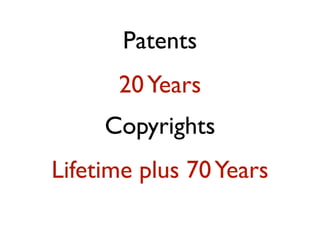


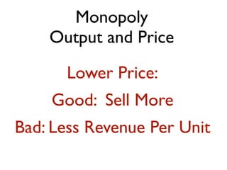


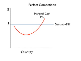


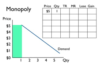


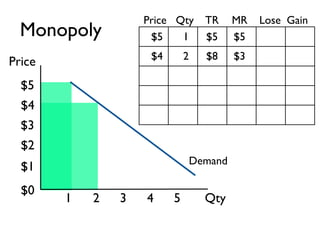


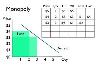


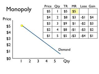


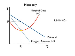

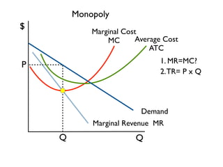

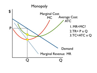


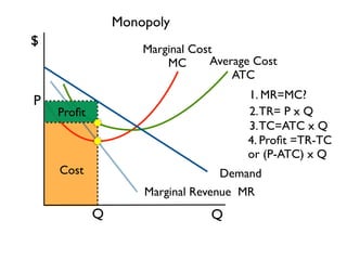


The document discusses the key differences between perfect competition and monopoly market structures. Under perfect competition, there are many small firms producing an identical product, while a monopoly has a single firm producing a unique product with barriers to entry. A monopoly faces a downward-sloping demand curve and must lower prices to increase quantity sold, unlike perfect competition where firms are price takers.


