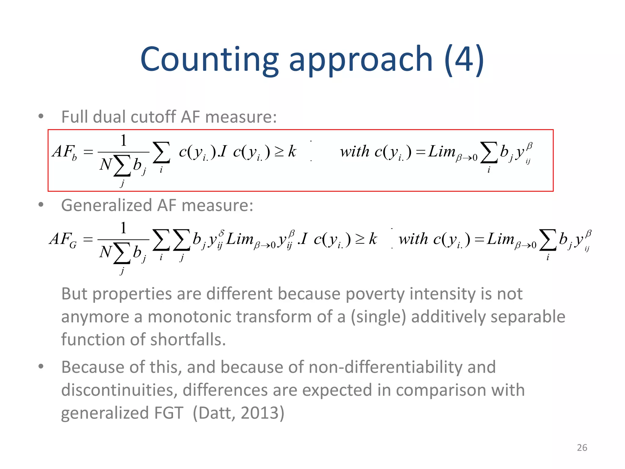
Multi-Dimensional Poverty
Measurement: where do we stand?
François Bourguignon
Paris School of Economics
Monash University, May 2013
1
Centre for Development Economics
presents
Multi-Dimensional Poverty
Measurement: where do we stand?
François Bourguignon
Paris School of Economics
Monash University, May 2013
2
Centre for Development Economics
presents
State of play
• Sen's impulse through the capability approach and the HDI
• Income imperfectly correlated with other dimensions of well-
being
• "Poverty is multi-faceted"
– How to measure it? Does it make sense to aggregate all its
dimensions into a single indicator? Isn't income poverty
sufficient?
– Does measurement yield information on how to reduce it?
• This presentation as a contribution to the debate
3
State of play (2)
The various approaches to measurement
• Purely statistical approaches (fuzzy sets, entropy, distance,..)
• Extension of normative poverty measures to two (or more)
dimensions (Tsui, 2002, Bourguignon-
Chakravarty, 2003, 2007, Duclos et al., 2006, ...)
• Counting approach and 'dual cut-off' presented as an alternative
(Alkire-Foster, 2011)
Practically:
• Increasing use of the dual cut-off approach, much less of the
normatively grounded measures
• At the same time, strong criticisms of the counting approach and of
the goal of summarizing multi-dimensional poverty into one single
number (Ravallion, 2011)
• Where do we stand as of now? Where should we go?
4
Outline
1. What kind of poverty do we want to measure?
2. A basic analytical framework
3. "Adding-up" dimensions: back to unidimensional
measures
4. Generalizing FGT and dominance criteria
5. Counting approach and the AF measure
6. Conclusion
5
1) What kind of poverty do we want to
measure?
1) Individual welfare
• Utility depends on: a) Market goods; b) Non-market goods (health
status, environment, security, ..)
• Poverty = inability to consume a minimum basket
• Market goods: monetary expenditure threshold (standard 'income'
poverty, price aggregation)
• Non-market goods: no price available, a minimum has to be
specified for each one of them …
• … or a locus in the space of goods (Duclos et al.)
• To what extent does non-market good consumption depend also
on income? (Imperfect correlation = preference heterogeneity ?)
6
Three ways to define the poverty area in the
goods space (2 dimensions)
7
xM
zM
xNM
zNM
Poverty
zNM(zM)
Union
Intersection
General
What do we want to measure? (cont'd)
2) The capability approach
• Set of possible functionings defined by:
assets, education, health, access to markets, justice, …
• Poverty defined by low levels of these capability determinants
• No price available to aggregate (except for wealth): minimum
endowment in each dimension or minimum of some
combination of them
3) Implications of the capability/well being distinction: make sure
that the framework underpinning the choice of multiple
dimensions is consistent.
– Money income and housing quality or money income and education
are inconsistent (except across countries for the latter).
8
2. Basic analytical framework: sequential
aggregation
• N individuals (i), J dimensions (j), "attributes" of i : xi.= (xij)
• Relative shortfall or deprivation in dimension j:
where zj = poverty line in dimension j
• Aggregate shortfall, or poverty intensity, for individual i:
• Aggregating across individuals, a poverty measure in the
sense of π is simply:
9
)/1,0( jijij zxMaxy
0)0(;0)(:)( .. iji yy
N
i
iy
N
P
1
. )(
1
Basic analytical framework (2)
A simple decomposition
• Poverty headcount in the sense of π:
• Average intensity of poverty among the poor:
• Therefore:
10
N
i
iyI
N
H
1
. 0)(
1
0)(
.
.
)(
1
iy
iy
H
P
PHP
Basic analytical framework (3)
Remarks:
• Order of aggregation steps:
– One might aggregate first the shorfalls across individuals and then
across dimensions: yet, this would be missing the joint distribution of
the various dimensions
• Comparing two distributions (yA and yB )
– Pπ comparison:
– Dominance criterion: e.g. A dominates B in the sense of Π.
11
withinallforBPAP ())()(
)(/)( BPAP
3. "Adding-up" dimensions: back to
unidimensional measures
Case where the function π is linear:
Then:
However:
Instead, Hπ is the proportion of people with at least one deprivation
(Union)
Multidimensional poverty thus appears as some linear combination
of unidimensional poverty measures
Roughly speaking: there is more poverty in A than in B if
unidimensional poverty is on average higher in A than in B
12
0,)(
1
. jij
J
j
ji byby
j
J
j
j PGbP .
1
j)dimensionin(headcount
1
J
j
z
j
j
HH
"Adding-up" dimensions (2)
The additive separability case:
Then:
The overall poverty index is a combination of unidimensional
poverty indices defined on the poverty intensity functions fj.
Example:
13
0(),0)0(,0,)()( '
1
. jjjijj
J
j
ji ffbyfby
j
f
J
j
j j
PbP .
1
0)( j
jj
ijijj forPPyyf
jjf
j
"Adding-up" dimensions (3)
Weight-dominance in the separability case:
Equivalent to:
In the additive separability case, there is less multi-
dimensional poverty in A than in B for all possible weights iff
poverty is smaller in A than in B for each dimension.
14
jallforbBPbBPAPbAP j
j
f
J
j
j
j
f
J
j
j jj
0)(.)()(.)(
11
jBPAP j
f
j
f jj
)()(
"Adding-up" dimensions (4)
Overall dominance in the additive separability case:
Equivalent to:
Overall (first-order) dominance of A over B requires (first-order)
unidimensional poverty dominance in all dimensions.
The same result applies for second-order dominance
IN SUMMARY: The additive separability of π makes multidimensional
poverty analysis equivalent to unidimensional poverty analysis in
each dimension.
The cross distribution of attributes does not matter!!
15
jfffbBPbBPAPbAP jjjjf
J
j
jf
J
j
j jj
0();0)0(:,0)()()()( '
11
jzvBHAH j
vv
jj
,)()( 11
"Adding-up" dimensions (5)
• Effect of a monotonically increasing transformation of an additively
separable individual poverty intensity function
It is now the case that:
• Taking a linear approximation leads to:
The joint distribution of the J attributes now matters
16
0()',0,0,)(
1
. jj
J
j
ji byby j
ij
jk
ijik
J
j i k
kjj yyb
N
bP )('
1
1
j
J
j
j j
PbP .
1
4. Generalizing FGT and dominance criteria
• In the case J=2, an interesting particular specification is:
which generalizes the familiar FGT or Pα measure: the α-
power of the β-power mean of the two shortfalls
(Bourguignon and Chakravarty).
• β determines the substitutability between the shortfalls of the
two attributes in defining the overall poverty intensity; α
measures the aversion to poverty; b the relative weight of the
two attributes.
17
1,0;0,)1(
1
2
,,
1
bybby
N
P
i
i
b
i
Generalizing FGT (2)
• In the case where the second attribute is discrete (0/1) with
z2=1 this measure becomes:
where nk is the proportion of the population with yi2 = k (=0/1).
Multidimensional poverty is a weigthed average of attribute 1's
Pα for the non-poor in attribute 2 and a 'modified Pα' for the
others.
The 'modified Pα' increases the poverty intensity for any
shortfall yi1 but at the declining rate with yi1.
18
11
1
2
10
2
11
1
1
1
0
i
ii
y
i
b
b
yy
nN
n
yP
N
n
Generalizing FGT (3)
• In the case where the two attributes are discrete (0/1) with
z2=1 the generalized FGT becomes:
where nkm is the number of individuals with yi1 = k (=0/1) and
yi2 = m (=0/1) .
19
/
01
/
1011 )1(.
1
bnbnn
N
Dominance criteria (1)
• (Bourguignon-Chakravarty, 2007, in the case J=2)
Let:
Theorem 1 (Union): Pπ(A) ≤ Pπ(B) for all π( ) in Π+ iff:
where is the two-dimensioned headcount
Theorem 2 (Intersection): Pπ(A) ≤ Pπ(B) for all π( ) in Π- iff:
20
0;0,:(.,.)
0;0,:(.,.)
2121
2121
yyyy
yyyy
2,1)()()()()()( 21212121
12211221 jzvBHBHBHAHAHAH jj
vvvvvvvv
21
12
vv
H
2,1)()(;2,1),()( 2121
1212 jzvBHAHjBHAH jj
vvvvv
j
v
j
jj
Dominance criteria (2)
21
Generalized FGT and dominance criteria (end)
• Π+ and Π- in the case of generalized FGT (Pα,β,b)
• Interestingly enough, this condition does not depend only on
the substitutability parameter β but also on the poverty
aversion parameter α.
• Other dominance result (Duclos et al., 2006), idem theorem 2
(intersection) for general shape of the poverty domain.
• Difficulty of using generalized FGT for J>2. Should the
susbtitutability be the same for all dimensions? Possibly of
using nested CES functions.
22
1/)1(() 21
iffybby ii
5. Counting approach and the AF measure
• One of the first approaches used in poverty measurement:
counting the number of deprivation
• Recently formalized by Alkire and Foster (2011) as 'dual
cutoff':
– First cutoff : poverty threshold in each dimension
– Second cutoff: poor = individuals deprived in k dimensions or more
(out of J)
• Interestingly enough, the AF measure can be obtained as a
non-linear transformation of the generalized FGT (along the
lines of Atkinson, 2003)
23
Counting approach (2)
• Basic property:
• Counting the number of deprivations among J:
• Dual cutoff: poor if at least k deprivations
• Headcount:
24
0)()1(0)(01,0 0 yiffyLimthenandyIf
0)(
1
.. kycI
N
H i
i
J
j
iji yyc
1
0. lim)(
Counting approach (3)
• Simple poverty intensity = average proportion of deprivations
• And, after introducing weights, for the various dimensions
• Poverty intensity = non-linear monotonic transformation of
additively separable function of shortfalls
• Poverty intensity = non-linear monotonic transform of poverty
intensity in Generalized FGT (α = β)
25
i
iiii ij
yLimycwithkycIyc
J
y )()().(
1
)( ....0
i
jiii
j
j
ib ij
ybLimycwithkycIyc
b
y )()().(
1
)( ....
Counting approach (4)
• Full dual cutoff AF measure:
• Generalized AF measure:
But properties are different because poverty intensity is not
anymore a monotonic transform of a (single) additively separable
function of shortfalls.
• Because of this, and because of non-differentiability and
discontinuities, differences are expected in comparison with
generalized FGT (Datt, 2013)
26
i
jiii
i
j
j
b ij
ybLimycwithkycIyc
bN
AF 0... )()().(
1
i
jiiij
i j
ijj
j
j
G ij
ybLimycwithkycIyLimyb
bN
AF 0..0 )()(.
1
Conclusion
General points
• Many indicators available to describe the average distance in
between an observation and a reference frontier (or point)
called 'poverty' in a multidimensional space
• Preference for those with an economic/normative
interpretation and generalizing known uni-dimensional
concepts
• Experience with application of available measures is key. Too
early to make judgements
• Overall context matters: what it is that we try to measure (e.g.
space of outcomes/capability)
27
Conclusion(2)
More specific points
• Common structure between straight generalizations of one-
dimensional measure, FGT type, and 'counting approach' (AF)
• Yet, properties likely to differ because more or less non-
linearity in transformation of a basic poverty-intensity (or
distance) function
• Nice decomposability properties in case of additive separable
function but covariance/copula not in the picture
• Decomposability properties lack transparency in other
cases, except with dominance criteria
• Policy application requires such decomposability w.r.t.
marginal distributions and copula
28
Conclusion(3)
Work is still ongoing…
After all, it took us a fair amount of time to master one-
dimensional poverty measurement!
29
30

Monash CDE Bourguignon Multidimentional Poverty Measurement

  • 1.
    Multi-Dimensional Poverty Measurement: wheredo we stand? François Bourguignon Paris School of Economics Monash University, May 2013 1 Centre for Development Economics presents
  • 2.
    Multi-Dimensional Poverty Measurement: wheredo we stand? François Bourguignon Paris School of Economics Monash University, May 2013 2 Centre for Development Economics presents
  • 3.
    State of play •Sen's impulse through the capability approach and the HDI • Income imperfectly correlated with other dimensions of well- being • "Poverty is multi-faceted" – How to measure it? Does it make sense to aggregate all its dimensions into a single indicator? Isn't income poverty sufficient? – Does measurement yield information on how to reduce it? • This presentation as a contribution to the debate 3
  • 4.
    State of play(2) The various approaches to measurement • Purely statistical approaches (fuzzy sets, entropy, distance,..) • Extension of normative poverty measures to two (or more) dimensions (Tsui, 2002, Bourguignon- Chakravarty, 2003, 2007, Duclos et al., 2006, ...) • Counting approach and 'dual cut-off' presented as an alternative (Alkire-Foster, 2011) Practically: • Increasing use of the dual cut-off approach, much less of the normatively grounded measures • At the same time, strong criticisms of the counting approach and of the goal of summarizing multi-dimensional poverty into one single number (Ravallion, 2011) • Where do we stand as of now? Where should we go? 4
  • 5.
    Outline 1. What kindof poverty do we want to measure? 2. A basic analytical framework 3. "Adding-up" dimensions: back to unidimensional measures 4. Generalizing FGT and dominance criteria 5. Counting approach and the AF measure 6. Conclusion 5
  • 6.
    1) What kindof poverty do we want to measure? 1) Individual welfare • Utility depends on: a) Market goods; b) Non-market goods (health status, environment, security, ..) • Poverty = inability to consume a minimum basket • Market goods: monetary expenditure threshold (standard 'income' poverty, price aggregation) • Non-market goods: no price available, a minimum has to be specified for each one of them … • … or a locus in the space of goods (Duclos et al.) • To what extent does non-market good consumption depend also on income? (Imperfect correlation = preference heterogeneity ?) 6
  • 7.
    Three ways todefine the poverty area in the goods space (2 dimensions) 7 xM zM xNM zNM Poverty zNM(zM) Union Intersection General
  • 8.
    What do wewant to measure? (cont'd) 2) The capability approach • Set of possible functionings defined by: assets, education, health, access to markets, justice, … • Poverty defined by low levels of these capability determinants • No price available to aggregate (except for wealth): minimum endowment in each dimension or minimum of some combination of them 3) Implications of the capability/well being distinction: make sure that the framework underpinning the choice of multiple dimensions is consistent. – Money income and housing quality or money income and education are inconsistent (except across countries for the latter). 8
  • 9.
    2. Basic analyticalframework: sequential aggregation • N individuals (i), J dimensions (j), "attributes" of i : xi.= (xij) • Relative shortfall or deprivation in dimension j: where zj = poverty line in dimension j • Aggregate shortfall, or poverty intensity, for individual i: • Aggregating across individuals, a poverty measure in the sense of π is simply: 9 )/1,0( jijij zxMaxy 0)0(;0)(:)( .. iji yy N i iy N P 1 . )( 1
  • 10.
    Basic analytical framework(2) A simple decomposition • Poverty headcount in the sense of π: • Average intensity of poverty among the poor: • Therefore: 10 N i iyI N H 1 . 0)( 1 0)( . . )( 1 iy iy H P PHP
  • 11.
    Basic analytical framework(3) Remarks: • Order of aggregation steps: – One might aggregate first the shorfalls across individuals and then across dimensions: yet, this would be missing the joint distribution of the various dimensions • Comparing two distributions (yA and yB ) – Pπ comparison: – Dominance criterion: e.g. A dominates B in the sense of Π. 11 withinallforBPAP ())()( )(/)( BPAP
  • 12.
    3. "Adding-up" dimensions:back to unidimensional measures Case where the function π is linear: Then: However: Instead, Hπ is the proportion of people with at least one deprivation (Union) Multidimensional poverty thus appears as some linear combination of unidimensional poverty measures Roughly speaking: there is more poverty in A than in B if unidimensional poverty is on average higher in A than in B 12 0,)( 1 . jij J j ji byby j J j j PGbP . 1 j)dimensionin(headcount 1 J j z j j HH
  • 13.
    "Adding-up" dimensions (2) Theadditive separability case: Then: The overall poverty index is a combination of unidimensional poverty indices defined on the poverty intensity functions fj. Example: 13 0(),0)0(,0,)()( ' 1 . jjjijj J j ji ffbyfby j f J j j j PbP . 1 0)( j jj ijijj forPPyyf jjf j
  • 14.
    "Adding-up" dimensions (3) Weight-dominancein the separability case: Equivalent to: In the additive separability case, there is less multi- dimensional poverty in A than in B for all possible weights iff poverty is smaller in A than in B for each dimension. 14 jallforbBPbBPAPbAP j j f J j j j f J j j jj 0)(.)()(.)( 11 jBPAP j f j f jj )()(
  • 15.
    "Adding-up" dimensions (4) Overalldominance in the additive separability case: Equivalent to: Overall (first-order) dominance of A over B requires (first-order) unidimensional poverty dominance in all dimensions. The same result applies for second-order dominance IN SUMMARY: The additive separability of π makes multidimensional poverty analysis equivalent to unidimensional poverty analysis in each dimension. The cross distribution of attributes does not matter!! 15 jfffbBPbBPAPbAP jjjjf J j jf J j j jj 0();0)0(:,0)()()()( ' 11 jzvBHAH j vv jj ,)()( 11
  • 16.
    "Adding-up" dimensions (5) •Effect of a monotonically increasing transformation of an additively separable individual poverty intensity function It is now the case that: • Taking a linear approximation leads to: The joint distribution of the J attributes now matters 16 0()',0,0,)( 1 . jj J j ji byby j ij jk ijik J j i k kjj yyb N bP )(' 1 1 j J j j j PbP . 1
  • 17.
    4. Generalizing FGTand dominance criteria • In the case J=2, an interesting particular specification is: which generalizes the familiar FGT or Pα measure: the α- power of the β-power mean of the two shortfalls (Bourguignon and Chakravarty). • β determines the substitutability between the shortfalls of the two attributes in defining the overall poverty intensity; α measures the aversion to poverty; b the relative weight of the two attributes. 17 1,0;0,)1( 1 2 ,, 1 bybby N P i i b i
  • 18.
    Generalizing FGT (2) •In the case where the second attribute is discrete (0/1) with z2=1 this measure becomes: where nk is the proportion of the population with yi2 = k (=0/1). Multidimensional poverty is a weigthed average of attribute 1's Pα for the non-poor in attribute 2 and a 'modified Pα' for the others. The 'modified Pα' increases the poverty intensity for any shortfall yi1 but at the declining rate with yi1. 18 11 1 2 10 2 11 1 1 1 0 i ii y i b b yy nN n yP N n
  • 19.
    Generalizing FGT (3) •In the case where the two attributes are discrete (0/1) with z2=1 the generalized FGT becomes: where nkm is the number of individuals with yi1 = k (=0/1) and yi2 = m (=0/1) . 19 / 01 / 1011 )1(. 1 bnbnn N
  • 20.
    Dominance criteria (1) •(Bourguignon-Chakravarty, 2007, in the case J=2) Let: Theorem 1 (Union): Pπ(A) ≤ Pπ(B) for all π( ) in Π+ iff: where is the two-dimensioned headcount Theorem 2 (Intersection): Pπ(A) ≤ Pπ(B) for all π( ) in Π- iff: 20 0;0,:(.,.) 0;0,:(.,.) 2121 2121 yyyy yyyy 2,1)()()()()()( 21212121 12211221 jzvBHBHBHAHAHAH jj vvvvvvvv 21 12 vv H 2,1)()(;2,1),()( 2121 1212 jzvBHAHjBHAH jj vvvvv j v j jj
  • 21.
  • 22.
    Generalized FGT anddominance criteria (end) • Π+ and Π- in the case of generalized FGT (Pα,β,b) • Interestingly enough, this condition does not depend only on the substitutability parameter β but also on the poverty aversion parameter α. • Other dominance result (Duclos et al., 2006), idem theorem 2 (intersection) for general shape of the poverty domain. • Difficulty of using generalized FGT for J>2. Should the susbtitutability be the same for all dimensions? Possibly of using nested CES functions. 22 1/)1(() 21 iffybby ii
  • 23.
    5. Counting approachand the AF measure • One of the first approaches used in poverty measurement: counting the number of deprivation • Recently formalized by Alkire and Foster (2011) as 'dual cutoff': – First cutoff : poverty threshold in each dimension – Second cutoff: poor = individuals deprived in k dimensions or more (out of J) • Interestingly enough, the AF measure can be obtained as a non-linear transformation of the generalized FGT (along the lines of Atkinson, 2003) 23
  • 24.
    Counting approach (2) •Basic property: • Counting the number of deprivations among J: • Dual cutoff: poor if at least k deprivations • Headcount: 24 0)()1(0)(01,0 0 yiffyLimthenandyIf 0)( 1 .. kycI N H i i J j iji yyc 1 0. lim)(
  • 25.
    Counting approach (3) •Simple poverty intensity = average proportion of deprivations • And, after introducing weights, for the various dimensions • Poverty intensity = non-linear monotonic transformation of additively separable function of shortfalls • Poverty intensity = non-linear monotonic transform of poverty intensity in Generalized FGT (α = β) 25 i iiii ij yLimycwithkycIyc J y )()().( 1 )( ....0 i jiii j j ib ij ybLimycwithkycIyc b y )()().( 1 )( ....
  • 26.
    Counting approach (4) •Full dual cutoff AF measure: • Generalized AF measure: But properties are different because poverty intensity is not anymore a monotonic transform of a (single) additively separable function of shortfalls. • Because of this, and because of non-differentiability and discontinuities, differences are expected in comparison with generalized FGT (Datt, 2013) 26 i jiii i j j b ij ybLimycwithkycIyc bN AF 0... )()().( 1 i jiiij i j ijj j j G ij ybLimycwithkycIyLimyb bN AF 0..0 )()(. 1
  • 27.
    Conclusion General points • Manyindicators available to describe the average distance in between an observation and a reference frontier (or point) called 'poverty' in a multidimensional space • Preference for those with an economic/normative interpretation and generalizing known uni-dimensional concepts • Experience with application of available measures is key. Too early to make judgements • Overall context matters: what it is that we try to measure (e.g. space of outcomes/capability) 27
  • 28.
    Conclusion(2) More specific points •Common structure between straight generalizations of one- dimensional measure, FGT type, and 'counting approach' (AF) • Yet, properties likely to differ because more or less non- linearity in transformation of a basic poverty-intensity (or distance) function • Nice decomposability properties in case of additive separable function but covariance/copula not in the picture • Decomposability properties lack transparency in other cases, except with dominance criteria • Policy application requires such decomposability w.r.t. marginal distributions and copula 28
  • 29.
    Conclusion(3) Work is stillongoing… After all, it took us a fair amount of time to master one- dimensional poverty measurement! 29
  • 30.

Editor's Notes

  • #7 Parallelwith GDP-extensions and Stiglitz-Sen commission
  • #9 Parallelwith GDP-extensions and Stiglitz-Sen commission