.

1. Effect of Coflow Turbulence on the Dynamics
and Mixing of a Nonbuoyant Turbulent Jet
Masoud Moeini1
; Babak Khorsandi2
; and Laurent Mydlarski3
Abstract: The effect of a turbulent coflow on a turbulent round jet is investigated experimentally. The primary objective of this work is to
study the evolution of the turbulent jet as the level of the coflow turbulence is varied. Velocity measurements of the jet were conducted at three
Reynolds numbers, with the jet issuing into two different levels of coflow turbulence. It is observed that the decay rate of the centerline mean
velocity, spreading rate, and mass flow rate of the jet increase as the level of the coflow turbulence increases. Similarly, both the inward mean
radial velocity close to the edges of the jet, which can be related to the entrainment velocity, and the velocity variances increase when the
turbulence level of coflow increases. Given the increased spreading rate, mass flow rate, and inward mean radial velocities, it can be inferred
that the entrainment into the jet also increases as the coflow turbulence intensifies. Lastly, for the range of parameters studied, self-similarity
of mean velocity profiles occurs at a downstream position for which the ratio of the coflow to jet integral lengthscales is of order one.
DOI: 10.1061/(ASCE)HY.1943-7900.0001830. © 2020 American Society of Civil Engineers.
Introduction
Interest in the mixing of both momentum and scalars in turbulent
jets or plumes arises mainly from their relevance to a wide range of
practical engineering applications. Examples include brine dispos-
als from desalination plants (Marti et al. 2011; Choi et al. 2016;
Abessi and Roberts 2017; Baum and Gibbes 2019) and acidic dis-
charges from exhaust gas scrubbers on ships (Ülpre et al. 2013), to
the release of municipal waste into shallow waters (Chowdhury
et al. 2017) and biogas emissions from deep reservoirs (He et al.
2018). The prevalence of jets to renewable-fuel applications, such
as nonreacting mixing of blends of synthetic biogas with air (Johchi
et al. 2019), and to applications involving air–fuel mixtures dis-
charging into combustion chambers in the form of coaxial jets
(Canton et al. 2017; Montagnani and Auteri 2019), are also espe-
cially important. Such examples underscore the importance of the
study of the impacts of such jet/plume-based releases, whether the
aim be to mitigate the detrimental effects of contaminants at high
concentrations in the environment or to improve mixing in indus-
trial applications.
In the aforementioned instances of jets/plumes discharging into
the atmosphere or aqueous environments, the ambient fluid is sel-
dom quiescent and is often characterized by a mean velocity. Three
distinct cases occur when the main direction of the flow of the sur-
rounding fluid is parallel, perpendicular, or opposite to the main
direction of the jet’s development. In these cases, the surrounding
flow is typically referred to as a “coflow” (Wright 1994), “crossflow”
(de Wit et al. 2014; Choi et al. 2016), or “counterflow” (Amamou
et al. 2015; Mahmoudi and Fleck 2016), respectively. The first is the
topic of the current study.
The dynamics of a nonbuoyant turbulent jet issued into a coflow
have been the subject of numerous studies. Various experimental
results show that the mean velocities of jets in coflows will become
independent of their initial conditions at far downstream distances
and only depend on the net momentum excess and local conditions,
such as the jet width and velocity excess. These results confirm the
notion of self-similarity of mean properties of a jet in a coflow
(Antonia and Bilger 1973; Smith and Hughes 1977; Nickels and
Perry 1996; Chu et al. 1999). Mean scalar concentrations of jets
emitted into coflows have also been shown to be approximately
self-similar (Chu et al. 1999; Davidson and Wang 2002). Chu et al.
(1999) observed that the widths of the velocity and concentration
fields vary nonlinearly with downstream distance. They presented
an integral model for mean quantities, such as the centerline min-
imum dilution. For higher-order moments, Antonia and Bilger
(1973) and Smith and Hughes (1977) observed that Reynolds
stresses were not self-similar and suggested that the assumption
of self-similarity in such flows was incorrect. In support of this
argument, it has been argued that the normalized root-mean
square (RMS) concentration fluctuations was self-similar close
to the jet, but then increased farther downstream, where self-
similarity was disrupted (Davidson and Wang 2002).
A set of the aforementioned experiments have been performed
in low-turbulence-intensity coflows (e.g., Antonia and Bilger 1973;
Nickels and Perry 1996), but some did not report any value of the
intensity of the coflow’s turbulence (e.g., Smith and Hughes 1977;
Chu et al. 1999). In this regard, some of the apparent inconsisten-
cies in past studies may be associated with the magnitude of the
turbulence that is present in coflows. Moreover, Davidson and
Wang (2002) suggested that the noticeable scatter in the measure-
ments from different studies of the jet’s spreading rate in the weakly
advected region was associated with the presence of ambient tur-
bulence in those experiments. They therefore designed their experi-
ments to minimize the impact of ambient turbulence.
Furthermore, the effect of coflow turbulence on the statistics of
turbulent jets is not included in most integral models. For instance,
1
Research Assistant, Dept. of Civil and Environmental Engineering,
Amirkabir Univ. of Technology (Tehran Polytechnic), 350 Hafez St.,
Tehran 15916-34311, Iran. Email: masoudm@aut.ac.ir
2
Assistant Professor, Dept. of Civil and Environmental Engineering,
Amirkabir Univ. of Technology (Tehran Polytechnic), 350 Hafez St.,
Tehran 15916-34311, Iran (corresponding author). ORCID: https://orcid
.org/0000-0003-4088-9740. Email: b.khorsandi@aut.ac.ir
3
Associate Professor, Dept. of Mechanical Engineering, McGill Univ.,
817 Sherbrooke St. West, Montréal, QC, Canada H3A 0C3. Email: laurent
.mydlarski@mcgill.ca
Note. This manuscript was submitted on January 22, 2020; approved on
July 17, 2020; published online on October 23, 2020. Discussion period
open until March 23, 2021; separate discussions must be submitted for in-
dividual papers. This paper is part of the Journal of Hydraulic Engineer-
ing, © ASCE, ISSN 0733-9429.
© ASCE 04020088-1 J. Hydraul. Eng.
J. Hydraul. Eng., 2021, 147(1): 04020088
Downloaded
from
ascelibrary.org
by
Auckland
University
Of
Technology
on
10/23/20.
Copyright
ASCE.
For
personal
use
only;
all
rights
reserved.

2. formulation of the spreading rate of a jet in a coflow via the integral
model of Chu et al. (1999) ignores the effect of coflow turbulence.
Wright (1994) was probably the first to note that the effect of co-
flow turbulence on the entrainment of turbulent jets was non-ne-
gligible. By analysis of experimental results from other studies,
Wright (1994) demonstrated that the dilution and entrainment rate
of a jet increases as a result of an increase in the turbulence intensity
of the coflow (which was increased by increasing the bed rough-
ness). He hypothesized that the mixing produced by the ambient
turbulence adds to the jet mixing and modified conventional inte-
gral models by adding a separate term to account for the ambient
turbulence. However, the model was tested against limited exper-
imental data from other studies.
On the other hand, Wright’s (1994) hypothesis is opposite to
that of Hunt (1994), who argued that background turbulence will
lower the entrainment velocities by breaking up the jet structure. A
decrease in the entrainment rate of a jet in a turbulent background
with zero mean flow was reported by Khorsandi et al. (2013) and
Lai et al. (2019) despite an observed increase in the jet dilution by
Perez-Alvarado (2016) and Afrooz (2019) in the same flow. Sim-
ilarly, Gaskin et al. (2004) also reported a decreased entrainment for
a plane jet in a shallow coflow.
Given the aforementioned shortcomings and inconsistencies,
an experimental investigation of the effect of coflow turbulence
on the dynamics and mixing of an axisymmetric turbulent jet was
conducted. Measurement of the mean and RMS velocities, veloc-
ity spectra, and centerline integral lengthscales were undertaken.
Furthermore, the effect of a turbulent coflow on the mixing and
entrainment into the jet will be inferred from the measurements
of jet’s width and mass flow rate. The present work provides a
novel database that covers various magnitudes of coflow turbulence
and jet-to-coflow velocity ratios, and their interplay in determining
the dynamics and mixing of the flow. In addition to furthering cur-
rent understanding of this class of flows, the measurements herein
will hopefully enable the testing and evaluation of models of such
flows.
The remainder of this paper is organized as follows. The exper-
imental apparatus and measurement techniques are first described,
followed by a discussion of the coflow characteristics, validation
of flow measurements, and flow parameterization. Experimental
results pertaining to measurements of turbulent jets issued into
turbulent coflows are then presented and discussed. Lastly, conclu-
sions are drawn.
Experimental Apparatus and Measurement
Techniques
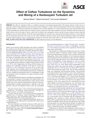
The experiments were conducted in the middle portion of a
6-m-long flume filled with water. Schematic diagrams of the setup
illustrating its top and side views are shown in Fig. 1. The width of
the flume was 0.5 m, and the water depth was maintained at 0.45 m
using a Plexiglas (polymethyl methacrylate) weir at the end of the
flume. Its bottom and side walls were made of toughened transparent
0.58
0.58
0.54
Rails
Coflow
Wooden-fiber blanket &
Plexiglas weir
Jet
ADV
x
y
Upstream basin
Curved contractions
1.5
6.0
2.0
Stilling
basin
(a)
(b)
Fig. 1. Schematic diagrams of the flume, ADV, and jet facility for the jet issuing into the coflow (not to scale): (a) top view; and (b) side view.
Dimensions are in meters.
© ASCE 04020088-2 J. Hydraul. Eng.
J. Hydraul. Eng., 2021, 147(1): 04020088
Downloaded
from
ascelibrary.org
by
Auckland
University
Of
Technology
on
10/23/20.
Copyright
ASCE.
For
personal
use
only;
all
rights
reserved.

3. glass. The water flowed from an upstream basin to the flume and
then overflowed into a downstream stilling basin. The flume was
connected to the upstream basin by way of a curved symmetric con-
traction and separated from the stilling basin by the Plexiglas weir
and flexible wooden-fiber blankets placed in front. The curved con-
tractions served to increase the uniformity and isotropy of the open-
channel flow. The wooden-fiber blankets led to a smooth overflow of
the channel flow into the stilling basin.
Two pumps maintained the circulation of water in the flume
by pumping the water from the stilling basin (via a 9-m-long,
0.031-m-diameter polyethylene pipe) back to the upstream basin.
Inhomogeneities in the flow of the water discharged into the up-
stream basin were minimized by passing the flow through perfo-
rated steel plate (resembling a honeycomb with a mesh size of
approximately 0.01 m), and by a number of wooden-fiber blan-
kets, prior to entering the flume. Moreover, an aluminium honey-
comb was used during the experiments, with its cross-sectional
size being the same as the width of the flume. Its thickness (in
the direction of the flow) and the wall thickness were 0.05 and
50 × 10−6
m, respectively, with a mesh size of 0.005 m.
Two turbulent open-channel flows with similar mean velocities,
but different turbulent kinetic energies (TKEs) were used in the
present experiments. The first level of coflow turbulence was that
of the flow downstream of the aforementioned honeycomb that was
placed at the inlet of the flume test section (i.e., the point at which
the contraction ends). The coflow in this scenario is called hereafter
the low-TKE coflow. Following the approach of Wright (1994), the
second level of coflow turbulence was produced by removing the
honeycomb and placing cohesionless aggregates of rounded sub-
angular fragments of rock with a nearly uniform distribution of
size (with d50 ¼ 0.015 m, referred to as gravel) on the flume’s bed.
The gravel bed was stable and completely fixed during the experi-
ments. The coflow in this scenario is referred to herein as the high-
TKE coflow. The coflow mean velocity (averaged through the cross
section) was 0.04 m=s for both the cases (i.e., with and without
gravel). To maintain the same mean coflow velocity for both sce-
narios, the flow rates of the circulation pumps were adjusted ac-
cordingly. The intensity of the coflow turbulence, defined herein
as the ratio of the axial RMS to mean velocity, was 3% and 7%
for the low- and high-TKE, respectively.
An axisymmetric turbulent jet of circular cross section was emit-
ted into the middle portion of the flume, parallel to the flume direc-
tion. The exit of the jet nozzle was fixed at a distance of 1.40 m from
the start of the test section, and the measurements were taken over the
range 45 ≤ x=D ≤ 105 (in the uniform potential core of the coflow),
where x is the distance from the jet nozzle, and D (=0.01 m) is the
diameter of the jet nozzle. The jet was fed from a constant-head tank
and precisely positioned by a traversing mechanism. The constant-
head tank consisted of a 0.1 m3-polyethylene container, supplied
with water from the stilling basin. Given its height of 2.8 m, jet
Reynolds numbers (Re ¼ UJD=ν, where UJ is the jet exit velocity,
and ν is the kinematic viscosity of water at 20°C) of up to 12,000
were obtained. The water level in the constant-head tank was main-
tained constant by an overflow that discharged the extra mass flow
rate back to the stilling basin. The temperature of the water in the jet
and that of the water into which it emerged were the same because
the jet was fed from the water of the flume.
The constant-head tank was connected by flexible tubing to a
0.01-m-diameter, L-shaped brass tube that comprised the jet. A
Georg Fischer d32 DN 25 (Schaffhausen, Switzerland) flowmeter
with measurement accuracy of 1%, in conjunction with a ball valve
located upstream of the flowmeter, maintained flow rates corre-
sponding to jet exit velocities of 0.7, 1.0, and 12 m=s and Reynolds
numbers of approximately 7.0 × 103, 10 × 103, and 12 × 103.
The velocity field was measured by a Nortek Vectrino Plus
(Rud, Norway) acoustic Doppler velocimeter (ADV). The Nortek
Vectrino Plus ADV measures velocities in x-, y- and z-directions.
Given that the present ADV provides two estimates of the velocity
in the z-direction, these can be used to find the contribution of noise
to velocity variances (Hurther and Lemmin 2001). When using the
ADV, procedures were undertaken to carefully align the ADV
probe with the centerline of the jet. The measurements were taken
across the flume’s width (at the middepth of the flume) to ensure
the symmetry of measurements. The accuracy of velocity measure-
ments was 0.5% of the measured values 1 mm=s (Nortek 2018).
To span the full range of measured velocities, ADV velocity ranges
of 10 and 30 cm=s were used.
During the measurements, the transmit pulse length and sam-
pling volume height were set to their maximum level (2.4 and
9.1 mm, respectively), which result in an increased signal-to-noise
ratio and reduced Doppler noise (Lohrmann et al. 1994; Nortek
2018). The sampling volume is located approximately 5 cm below
the ADV transmitter (Nortek 2018), resulting in minimal flow dis-
turbance by the probe. Furthermore, talcum powder was added to
the flow (and was mixed every few hours) to ensure high signal-to-
noise ratios of the measurements (Khorsandi et al. 2012). The
ADV’s sampling frequency was set to its maximum value, 200 Hz,
and measurements were made for a duration of 8 min to ensure
convergence of the statistics up to the fourth order.
The signal quality was high for all measurements, i.e., the
signal-to-noise ratio and correlation were above 21% and 82%, re-
spectively, in the present laboratory flow. Therefore, despiking the
data did not significantly change the statistics. However, all ADV
measurements suffer from Doppler noise, which is inherent to the
technique and affects RMS velocities. The RMS velocities of the
coflow measured using the ADV in this study were postprocessed
using an accuracy-improvement technique developed by Moeini
et al. (2020). The technique is based on the simultaneous removal
of the effects of Doppler noise and velocity-variance damping,
where the former is calculated using the method of Hurther and
Lemmin (2001). Moreover, the measurements of turbulent jets
embedded in turbulent coflows are improved by way of the tech-
nique proposed by Khorsandi et al. (2012), which is based on the
symmetry of statistical measurements in two perpendicular direc-
tions, whose measurements exhibit an artificial difference resulting
from the different noise levels of the instrument along its differ-
ent axes.
Coflow Characteristics, Validation of Flow
Measurements, and Flow Parameterization
Before describing the main results pertaining to the statistics of the
turbulent jet, the statistics of the coflow into which the jet was re-
leased will be outlined. The flow conditions and relevant flow
parameters are summarized in Table 1. Here, U∞ is the mean co-
flow velocity, and urms, vrms, and wrms are RMS velocities in the x-,
y-, and z-directions, respectively. Statistics quantified in Table 1 are
measured in the downstream direction on the horizontal plane pass-
ing through the middepth of the flume, with which the centerline of
the jet was subsequently aligned. The axial decay of RMS veloc-
ities are reasonably insignificant over the range of downstream dis-
tances studied herein (e.g., Tavoularis and Corrsin 1981), and the
present study’s results confirm this to a high degree. The statistics
in the transverse direction were typical of those given in Table 1.
As established in Table 1, the mean coflow velocity, U∞, ex-
hibits good uniformity for the low-TKE coflow (5% ≈ 2.1=42)
and high-TKE coflow (1.0% ≈0.4=43), over the range of
© ASCE 04020088-3 J. Hydraul. Eng.
J. Hydraul. Eng., 2021, 147(1): 04020088
Downloaded
from
ascelibrary.org
by
Auckland
University
Of
Technology
on
10/23/20.
Copyright
ASCE.
For
personal
use
only;
all
rights
reserved.

4. downstream distances considered. Moreover, measurements of the
RMS velocities also suggest reasonable homogeneity and isotropy
of the coflow for a given level of TKE. Furthermore, because the
RMS velocities of coflows are one to two orders of magnitude
smaller than those of the jets, it is expected that the small degree
of anisotropy in the coflows does not significantly influence the
jets. The turbulence intensity (TI ≡ urms=U∞), the turbulent kinetic
energy per unit mass [TKE ≡ ðu2
rms þ v2
rms þ w2
rmsÞ=2], and the in-
tegral lengthscale of the coflow are also reported. The integral
lengthscale (l) is calculated using Taylor’s hypothesis: l ¼ U∞ ×
ITS (Tennekes and Lumley 1972; Sirivat and Warhaft 1983;
Mydlarski and Warhaft 1996), where ITS [≡∫ first zero
0 ρuðτÞdτ] is
the integral timescale obtained by integrating the autocorrelation
function (ρu) up to its first zero (Sirivat and Warhaft 1983).
Before conducting the main experiments, the ADV measure-
ments were validated in a turbulent jet issuing into a quiescent
background and compared against other studies, including ones
employing flying hot-wire anemometry (FHWA) (Panchapakesan
and Lumley 1993), stationary hot-wire anemometry (SHWA)
(Wygnanski and Fiedler 1969), and laser Doppler anemometry
(LDA) (Hussein et al. 1994; Darisse et al. 2015). Fig. 2 depicts
the radial profiles of mean axial velocity normalized by the mean
centerline axial velocity (Ucl) and the variance of the axial veloc-
ities normalized by the square of the centerline mean velocity.
The present data are consistent with those of other studies, which
serves to validate the apparatus and ADV measurements em-
ployed in the present work. A thorough set of benchmarking re-
sults were presented by Moeini et al. (2020).
Because this paper’s objective is to study the evolution of a tur-
bulent axisymmetric jet issued into a coflow as a function of coflow
turbulence, the results are reported in terms of the relative turbulent
kinetic energy (RTKE), defined as follows:
RTKE ≡
TKEC
TKEJ
ð1Þ
where TKEC = turbulent kinetic energy per unit mass of the coflow;
and TKEJ = turbulent kinetic energy per unit mass of the jet in
coflow. RTKE is a function of the downstream distance, whereas
low- and high-TKE refer only to the coflow and are independent
of the downstream distance. In conformity with Antonia and Bilger
(1973) and Nickels and Perry (1996), the nondimensional velocity
excess is defined by
λJ ≡
UJ − U∞
U∞
ð2Þ
as depicted in Fig. 3, along with the jet and coflow velocities. For λJ ≪
1 and λJ ≫ 1, the flow tends to a self-similar pure wake and pure jet,
respectively (Antonia and Bilger 1973). This study considers only val-
ues of λJ larger than unity, i.e., strong jets. Also, the momentum length
of the flow, lm, is defined as follows (Nickels and Perry 1996; Chu et al.
1999; Davidson and Wang 2002; Xia and Lam 2009):
lm ≡ M1=2
e =U∞ ð3Þ
where the excess momentum of the jet is
Table 1. Coflow statistics measured in the downstream direction (over the range where the jet statistics were measured) for the low- and high-turbulent kinetic
energy coflows
Coflow TKE level U∞ (mm=s) urms (mm=s) vrms (mm=s) wrms (mm=s) TI ≡ urms=U∞ × 100 TKE (mm2
=s2
) l (mm)
Low-TKE (45 ≤ x=D ≤ 95) 42 2.1 1.4 0.3 2.0 0.6 1.2 0.1 3.2 0.8 3.9 1.3 18 3
High-TKE (45 ≤ x=D ≤ 105) 43 0.4 3.0 0.3 2.4 0.4 2.9 0.2 7.0 0.7 11.9 2.4 30 5
(a) (b)
Fig. 2. Normalized radial profiles of (a) mean axial velocity; and (b) variance of the axial velocity of the turbulent jet issued into quiescent back-
ground (at x=D ¼ 75) and compared with results of other studies.
Fig. 3. Properties of the jet issued into a coflow.
© ASCE 04020088-4 J. Hydraul. Eng.
J. Hydraul. Eng., 2021, 147(1): 04020088
Downloaded
from
ascelibrary.org
by
Auckland
University
Of
Technology
on
10/23/20.
Copyright
ASCE.
For
personal
use
only;
all
rights
reserved.

5. Me ≡
Z ∞
0
UðU − U∞Þ2πrdr ð4Þ
where U ¼ UðrÞ = axial velocity; and r = radial position from the
centerline.
To normalize the downstream distance, alternative length-
scales (including the ones based on the coflow turbulence char-
acteristics) were investigated in this study; lm was found to be
the most appropriate lengthscale because it best fitted the data
at various values of λJ. In addition, lm is essentially independent
of downstream distance (Smith and Hughes 1977; Chu et al.
1999).
The characteristic lateral lengthscale of the jet may be defined
by the radius of gyration of the axial mean velocity excess about
r ¼ 0, which gives a measure of the distribution of velocity about
the centerline (Townsend 1976)
Δ ¼
R∞
0 r2ðU − U∞Þdr
R∞
0 ðU − U∞Þdr
1=2
ð5Þ
where Δ ≈ 0.849 × r1=2 ≈ 0.707 × r1=e, where r1=2 and r1=e
denote the radial distances at which the mean velocity excess
falls to half and 1=e of its centerline value, respectively, assum-
ing that the mean velocity excess profile has a Gaussian
distribution.
Results and Discussion
The flow parameters characterizing the present experiments are
given in Table 2. Overall, RTKE increases and Rl ≡ lC=lJ (where
lC is the integral lengthscale of the coflow and lJ is the integral
lengthscale of the jet issued into the coflow) decreases as the down-
stream distance increases. It is expected that when RTKE and Rl ∼
Oð1Þ [where Oð·Þ denotes order of magnitude], the jet structure
changes and jet breaks up into distinct eddies (Hunt 1994; Khorsandi
et al. 2013; Perez-Alvarado 2016).
The downstream decay of the mean axial centerline velocity
excess, U0 (≡Ucl − U∞), normalized by the mean coflow velocity
is plotted in Fig. 4 as a function of x=D [Fig. 4(a)] and x=lm
[Fig. 4(b)]. Measurements are made for both turbulent coflows con-
sidered and for λJ ¼ 16, 23, and 28, over the range 45 ≤ x=D ≤ 105.
Also plotted in Fig. 4(b) are the data of Nickels and Perry (1996),
Chu et al. (1999), and Davidson and Wang (2002).
It can be observed that the magnitude of mean velocity de-
creases in Fig. 4(a) with increasing the TKE of the coflow. Over
the full range of downstream distances considered, the data in
Fig. 4(a) are well described by power laws: U0=U∞ ¼ Aðx=DÞ−n.
A summary of the best-fit scaling exponents (n) are given in Table 3.
For a given λJ, the data corresponding to high-TKE coflow have
higher decay exponents. This trend is consistent with those ob-
served by Khorsandi et al. (2013) for a turbulent jet issued into
homogeneous isotropic turbulence with negligible mean flow.
Table 2. Flow parameters measured on the jet centerline corresponding to different jet Reynolds numbers over the range 45 ≤ x=D ≤ 105 and for the two
different turbulent coflows considered
Coflow TKE level λJ Re lm=D
x=D ¼ 55 x=D ¼ 70 x=D ¼ 85
RTKE Rl RTKE Rl RTKE Rl
Low-TKE 16 7,000 15.4 0.006 1.4 0.009 1.3 0.014 0.9
23 10,000 23.0 0.003 1.3 0.004 1.0 0.006 0.8
28 12,000 27.4 0.002 1.1 0.003 0.9 0.004 0.7
High-TKE 16 7,000 15.4 0.016 1.4 0.024 1.3 0.037 0.8
23 10,000 23.0 0.007 2.0 0.012 1.3 0.017 1.1
28 12,000 27.4 0.005 2.0 0.008 1.3 0.012 1.0
(a) (b)
Fig. 4. Variation of the centerline axial mean velocity excess measured for the two levels of coflow turbulence as a function of (a) x=D in linear-linear
coordinates; and (b) x=lm in log-log coordinates.
© ASCE 04020088-5 J. Hydraul. Eng.
J. Hydraul. Eng., 2021, 147(1): 04020088
Downloaded
from
ascelibrary.org
by
Auckland
University
Of
Technology
on
10/23/20.
Copyright
ASCE.
For
personal
use
only;
all
rights
reserved.

6. One concludes that higher turbulence levels of the coflow result in
lower axial mean velocity excesses and higher decay exponents.
When plotted as a function of x=lm, good collapse of the differ-
ent data sets is observed in Fig. 4(b). A decay exponent of approx-
imately −1 is consistent with other measurements for x=lm 10
(Nickels and Perry 1996; Chu et al. 1999; Or et al. 2011). With
increasing downstream distance, the difference between the mea-
surements recorded in the low and high levels of coflow turbulence
increases slightly. This is presumably due to an increase in RTKE at
the far downstream locations for which the effect of the turbulent
coflow is dominant. In this region, U0 is measurably smaller in the
presence of high-TKE coflow than when issued into the low-TKE
coflow.
Another important observation is that the magnitude of U0=U∞
obtained from the present measurements is slightly lower than that
reported by Nickels and Perry (1996) for the entire range of down-
stream distances considered. Nickels and Perry (1996) conducted
experiments in a coflow with negligible turbulence intensity, and
consequently, their centerline velocities were larger.
The radial profile of normalized axial mean velocity excess is
plotted as a function of r=Δ in Fig. 5, together with that reported
by Nickels and Perry (1996) for 2 ≤ λJ ≤ 20 over the range
30 ≤ x=D ≤ 90. At a given downstream distance, one observes that
the relative variation of the measurements for the two levels of co-
flow turbulence decreases with increasing λJ. This is attributed to
the decreasing value of RTKE with increasing λJ. For λJ ¼ 28 and
x=D ¼ 85, the profile measurements in both coflows become con-
sistent with the self-similar profile of Nickels and Perry (1996) as
reported for different downstream locations.
Given the radial profiles of axial velocity (Fig. 5), profiles of
V=U0 can be readily obtained from the integration of continuity
equation (Panchapakesan and Lumley 1993; Darisse et al. 2015).
Such profiles are plotted in Fig. 6 for both levels of coflow turbu-
lence and various λJ at different values of x=D. An important ob-
servation is that the coflow turbulence increases the magnitude of
V=U0 close to the edge of the jet (r=Δ 2). Because the entrain-
ment velocity [i.e., the inward velocity by which the ambient fluid
is drawn toward the center of the shear flow (e.g., Hunt 1994)] is
associated with the inflow at the edge of the turbulent jet, it is rea-
sonable to conclude that the entrainment velocity increases with
increasing coflow turbulence. Physically, one could expect that rel-
atively larger volumes of ambient fluid are drawn into the jet region
through an enhanced engulfment process as the TKE of the coflow
increases. This, in turn, can be expected to increase the levels of
mixing into the jet per unit surface area (of the outer edge). Con-
sequently, the dilution of jet fluid increases with increasing the co-
flow turbulence. Fig. 6 also indicates that with increasing λJ, the
relative deviations of the measurements close to the edge of the jet
for the low- and high-TKE coflows tend to drop, which is expected
given that larger values of RTKE are associated with lower values
of λJ.
Also of particular interest is how the lateral extent of the jets,
characterized by Δ, are affected by the presence of a turbulent
coflow. If one assumes that the spreading rate of a jet issued into
a coflow at sufficiently high λJ will asymptote to that of a jet issued
into a quiescent background (Davidson and Wang 2002), it is rea-
sonable to assume Δ ∼ x for the present measurements [by analogy
with the dynamics of a turbulent jet recorded in a stagnant environ-
ment (Townsend 1976)]. Table 4 lists a summary of the parameters
obtained by least-squares regression to an expression of the form
Δ=D ¼ S × ðx=DÞ þ S0 for various λJ and levels of coflow turbu-
lence. One observes that the spreading rate of the jet, Sð≡dΔ=dxÞ,
increases with increasing RTKE. This observation is consistent with
the results of Khorsandi et al. (2013) for an axisymmetric jet issued
into a homogeneous isotropic turbulence with zero mean flow. The
concentration measurements of Perez-Alvarado (2016) and Afrooz
(2019) also confirm this picture. The increase in the spreading rate
of the jet could increase mixing and dilution because it in turn in-
creases the mass flow rate (to be discussed subsequently).
A plot of Δ=lm versus x=lm for various Reynolds numbers and
both levels of coflow TKE is shown in Fig. 7. The curve fit to the
data of Nickels and Perry (1996) for λJ ¼ 10 and 20 is also plotted
for comparison. One observes that data for the lower TKE level lie
on a straight line, whereas there is some scatter in the case of high-
TKE coflow. The explanation is presumably that any possible self-
similarity is disrupted as the TKE of coflow increases. It can also be
seen that the spreading rate of the jet in the presence of the turbulent
coflow is higher than that of the jet in a coflow with negligible TKE
measured by Nickels and Perry (1996). This again implies an in-
crease in the mixing and dilution by the coflow turbulence.
To study the evolution of the mass flow rate (ṁ), one may em-
ploy the following equation, which is derived using control volume
analysis:
ṁ ¼ 2πρΔ2U0
Z ∞
0
r
Δ
f̄
r
Δ
d
r
Δ
ð6Þ
where f̄ ≡ ðUðr=ΔÞ − U∞Þ=U0 is the profile of normalized mean
velocity excess, as depicted in Fig. 5; and ρ = density of the fluid.
For a nonbuoyant jet in a quiescent background, ṁ varies linearly
with x (Pope 2000), and it is therefore reasonable to use linear fits
given that this asymptotic case is valid for a jet in a coflow for large
values of λJ. A summary of the best-fit lines to ṁ=ṁ0 data, where
ṁ0 ≡ πD2
ρUJ=4 is the initial mass flow rate, is given in Table 5.
Overall, one observes that the coflow turbulence tends to in-
crease the entrainment rates, dṁ=dx (¼ Eṁ0=D). Part of this in-
crease may be due to an increase in the spreading rate of the jet in
the presence of external turbulence, as expected from the definition
of mass flow rate, which accounts for the jet’s width. The increase
in the entrainment rates with increasing RTKE presumably enhances
the mixing and dilution. The present trend is consistent with the
increased magnitudes of V at the edge of the jet (which should
be correlated with the entrainment velocity) in the presence of co-
flow turbulence, as depicted in Fig. 6.
Hunt (1994) theoretically argued that weak external turbulence
does not significantly affect the entrainment velocities, whereas
strong external turbulence could disrupt the jet structure, resulting
in a decreased inward entrainment velocity, and therefore, de-
creased entrainment into the jet. The observations from the present
study, however, are different from the theoretical arguments of
Hunt (1994) for weak external turbulence. The present results point
to the conclusion that, assuming small enough values of RTKE
[∼Oð0.01Þ] so that the jet structure does not get disrupted, the co-
flow turbulence acts to increase the entrainment velocity as well as
both the spreading and entrainment rate of the jet. However, this
mechanism could change for larger values of RTKE.
The Eulerian temporal velocity spectra of the axial and vertical
velocities of a jet issued into both a turbulent coflow and a quiescent
Table 3. Summary of the best fit coefficients (A) and scaling exponents (n)
for the power laws U0=U∞ ¼ Aðx=DÞ−n
Coflow TKE level
λJ ¼ 16 λJ ¼ 23 λJ ¼ 28
A n A n A n
Low-TKE 73.4 0.94 134.3 0.98 183.8 1.00
High-TKE 101.0 1.03 186.1 1.06 251.7 1.08
© ASCE 04020088-6 J. Hydraul. Eng.
J. Hydraul. Eng., 2021, 147(1): 04020088
Downloaded
from
ascelibrary.org
by
Auckland
University
Of
Technology
on
10/23/20.
Copyright
ASCE.
For
personal
use
only;
all
rights
reserved.

7. background (measured at the centerline at x=D ¼ 105) are plotted
in Fig. 8. The velocity spectra of the high-TKE coflow (with no jet)
are also shown as a reference. For the two velocity components (u
and w), the spectra of turbulent jets issued into quiescent back-
grounds and coflow are similar in shape, but the latter have slightly
higher values, as expected from their relatively larger velocity var-
iances [which are equal to the area under the EðfÞ curves], to be
discussed subsequently. The relatively good consistency between the
spectra of the coflow (particularly, in the vertical direction) and the
general −5=3 power-law spectrum is apparent from the figure.
Fig. 9 depicts the variations of the centerline axial [Figs. 9(a
and b)] and vertical velocity variance [Figs. 9(c and d)], normalized
by the square of centerline excess velocity, as a function of x=D
and x=lm. Data are shown for different downstream locations and
for various jet Reynolds numbers. The measurements of Antonia and
Bilger (1973) and Nickels and Perry (1996) (with negligible RTKE)
are also presented for comparison. The axial and vertical velocity
variances are found to increase with increasing TKE of the coflow.
The overall magnitudes of the data suggest that the coflow turbulence
has a more significant effect for the lowest λJ (e.g., λJ ¼ 16), for
which RTKE is maximized. One expects that the increase in the nor-
mal components of Reynolds stress tensor lead to increased turbulent
mixing.
One can conclude from Fig. 9 that the constancy (i.e., self-
similarity) of the axial and vertical velocity variances for the high-
TKE data is disrupted, whereas the low-TKE data show a relatively
(a) (b)
(c) (d)
(e) (f)
Fig. 5. Radial profiles of axial mean velocity excess (normalized by the centerline excess velocity) measured for various values of λJ and x=D for the
two levels of coflow turbulence considered. The curve fit to the data of Nickels and Perry (1996) for λJ ¼ 2, 10, and 20 at x=D ¼ 30 [which is typical
of that for λJ ¼ 10 over the broad range 30 ≤ x=D ≤ 90 (see their Figs. 7 and 8)] is also plotted for comparison.
© ASCE 04020088-7 J. Hydraul. Eng.
J. Hydraul. Eng., 2021, 147(1): 04020088
Downloaded
from
ascelibrary.org
by
Auckland
University
Of
Technology
on
10/23/20.
Copyright
ASCE.
For
personal
use
only;
all
rights
reserved.

8. higher degree of similarity over the range of downstream distances
considered. The disruption of self-similarity appears to be more
notable at lower jet Reynolds numbers, for which RTKE is larger.
The relative invariance of the present measurements of axial veloc-
ity variance in a low-TKE coflow is consistent with the trend of the
data of Nickels and Perry (1996), measured in a flow of negligible
RTKE. Moreover, for the high-TKE coflow, the difference between
measurements for different values of λJ are higher than when
compared with the case of the low-TKE coflow. This may suggest
the existence of a nonlinear interplay between Re and RTKE in
(a) (b)
(c) (d)
(e) (f)
Fig. 6. Radial profiles of lateral mean velocity (normalized by the centerline excess velocity) calculated for various values of λJ and x=D and for the
two levels of coflow turbulence considered.
Table 4. Downstream variations of the jet’s width normalized by the diameter of the nozzle [Δ=D ¼ S × ðx=DÞ þ S0] for the two levels of coflow turbulence
considered
Coflow TKE level
λJ ¼ 16 λJ ¼ 23 λJ ¼ 28
S S0 S S0 S S0
Low-TKE 0.040 0.72 0.057 0.24 0.066 −0.087
High-TKE 0.064 −0.62 0.073 −1.33 0.081 −1.58
© ASCE 04020088-8 J. Hydraul. Eng.
J. Hydraul. Eng., 2021, 147(1): 04020088
Downloaded
from
ascelibrary.org
by
Auckland
University
Of
Technology
on
10/23/20.
Copyright
ASCE.
For
personal
use
only;
all
rights
reserved.

9. determining the magnitude of Reynolds stress tensor components.
Direct numerical simulation (DNS) for higher RTKE and higher
Reynolds numbers could shed light on the exact behavior of this
nonlinear effect.
Table 6 compares the centerline velocity variances with those of
previous studies. Where a range of downstream distances is specified,
the reported velocity variance is an average of variances in the self-
similar range. It can be seen that the velocity variances for strong
jets (large λJ) issued into negligible or low-TKE coflows are sim-
ilar to those of jets issued into a quiescent background. However,
the velocity variances for strong jets issued into a high-TKE coflow
and for weak jets (small λJ) released into a negligible coflow are
much higher than those of jets issued into a quiescent background.
The data of Smith and Hughes (1977) measured at x=D ¼ 40 have
not yet reached their asymptotic values and are therefore lower than
those of the other weak coflowing jets.
Fig. 10 plots the radial profiles of axial [Figs. 10(a and b)] and
vertical [Figs. 10(c and d)] components of velocity variance, nor-
malized by the square of centerline excess velocity, at two down-
stream locations: x=D ¼ 55 and x=D ¼ 85. The data of Antonia
and Bilger (1973) for flows of low RTKE are also plotted for com-
parison. One observes that the velocity variance increases with in-
creasing RTKE at a given λJ, especially close to the centerline. As a
result, it is reasonable to assume the turbulent mixing and dilution
across the radial profile should be enhanced as the TKE of the co-
flow increases.
From Fig. 10, one concludes that the effect of external turbu-
lence appears to be more significant close to the centerline because
the difference between low- and high-TKE-coflow measurements
decreases with the radial distance. The authors emphasize that the
aforementioned trend was also observed when using other renorm-
alizations (e.g., u2
rms=U2
∞). For u2
rms [Figs. 10(a and b)], there is
reasonable agreement between the current measurements and the
results of Antonia and Bilger (1973) for x=D ¼ 38, whereas those
measured therein at x=D ¼ 152 are higher. This can probably be
explained by the fact that the effect of coflow turbulence in that
study dominates at far downstream locations.
Fig. 11 depicts the radial profiles of local turbulence intensity
measured at x=D ¼ 70 for λJ ¼ 16 and 28 and for the two levels of
coflow turbulence in this study. The profile of turbulence intensity
for a jet issued into a quiescent background is also plotted for com-
parison. One observes that the evolution of the turbulence intensity
for a jet issued into a quiescent background is significantly different
from that of a jet issued into a coflow. The former grows infinitely
large as r → ∞, whereas the latter remains finite throughout the
jet’s lateral extent due to the existence of the coflow of finite tur-
bulence intensity. The profiles peak at a point [denoted as
ðr=ΔÞmax] between the centerline and the edge of the jet, which
Fig. 7. Variation of Δ with downstream distances and compared with
results of Nickels and Perry (1996). The present data are fit to the func-
tion Δ=lm ¼ S0
× ðx=lmÞ þ S0
0.
(a) (b)
Fig. 8. (a) Axial (u); and (b) vertical (w) velocity spectra measured at the jet centerline at x=D ¼ 105 for a jet issued into a quiescent background and
into the high-TKE coflow. A plot of the power spectra of u and w for the high-TKE coflow (alone) is also shown.
Table 5. Downstream evolution of the normalized mass flow rate
[ṁ=ṁ0 ¼ E×ðx=DÞþE0] of an axisymmetric turbulent jet issued into a
coflow
Coflow TKE level
λJ ¼ 16 λJ ¼ 23 λJ ¼ 28
E E0 E E0 E E0
Low-TKE 0.076 0.16 0.122 0.20 0.121 1.11
High-TKE 0.125 −2.25 0.170 −4.0 0.158 −2.28
Note: ṁ0 = initial mass flow rate: ρUJðπD2
=4Þ.
© ASCE 04020088-9 J. Hydraul. Eng.
J. Hydraul. Eng., 2021, 147(1): 04020088
Downloaded
from
ascelibrary.org
by
Auckland
University
Of
Technology
on
10/23/20.
Copyright
ASCE.
For
personal
use
only;
all
rights
reserved.

10. may depend on λJ, as seen in the figure. For r=Δ ðr=ΔÞmax, the
relative difference between low- and high-TKE coflows are small.
However, beyond ðr=ΔÞmax, there is a rather sharp decrease in the
turbulence intensity in the low-TKE coflow.
Lastly, the longitudinal integral lengthscale (l) measured at the
centerline of the jet is plotted as a function of x=D in Fig. 12(a) and
x=lm in Fig. 12(b). Here, the integral lengthscale is calculated as
l ¼ U × ITS where U is the mean axial velocity (Antonia and
Bilger 1973). The measurements are for a turbulent jet issued into
low- and high-TKE coflows at λJ ¼ 16, 23, and 28, as well as for
the low- and high-TKE coflows alone. A plot of the centerline
variation of the longitudinal integral lengthscale obtained by
(a) (b)
(c) (d)
Fig. 9. Downstream variations of the (a and b) axial; and (c and d) vertical velocity variances. These are shown as a function of x=D in plots (a) and
(c) and of x=lm in plots (b) and (d). Data of Nickels and Perry (1996) and Antonia and Bilger (1973) are also plotted for comparison.
Table 6. Parameters of jets issuing into coflows
References Jet background Measurement range λj u2
rms=U2
0 w2
rms=U2
0
Moeini et al. (2020) Quiescent 45 ≤ x=D ≤ 105 ∞ 0.060 0.032
Present study Coflow (low-TKE) 45 ≤ x=D ≤ 105 16 0.063 0.039
23 0.065 0.039
28 0.064 0.039
Coflow (high-TKE) 45 ≤ x=D ≤ 105 16 0.098 0.053
23 0.085 0.048
28 0.078 0.044
Nickels and Perry (1996) Coflow x=D ¼ 90 2 0.075 0.066
10 0.080 0.063
20 0.068 0.048
Smith and Hughes (1977) Coflow x=D ¼ 40 0.75 0.063 0.052
2.5 0.078 —
Antonia and Bilger (1973) Coflow 70 ≤ x=D ≤ 270 2 0.243 —
3.5 0.107 —
Note: Velocity variances are those on the centerline and averaged over the measurement range.
© ASCE 04020088-10 J. Hydraul. Eng.
J. Hydraul. Eng., 2021, 147(1): 04020088
Downloaded
from
ascelibrary.org
by
Auckland
University
Of
Technology
on
10/23/20.
Copyright
ASCE.
For
personal
use
only;
all
rights
reserved.

11. Wygnanski and Fiedler (1969) for a jet issued into quiescent back-
ground is also shown in Fig. 12(a), along with two power-law fits to
the data in Fig. 12(b).
From Fig. 12(a), one observes that l=D increases almost linearly
with downstream distance until x=D ¼ 85, at which all graphs
plateau and reach a constant value. The asymptotic values for l
of a jet issued into low- and high-TKE coflows (at sufficiently high
downstream locations) are similar to l values of the low- and high-
TKE coflows, respectively. The small deviations may be due to
uncertainties involved in the application of Taylor’s hypothesis.
(a) (b)
(c) (d)
Fig. 10. Radial profiles of axial and vertical velocity variances (normalized by the square of centerline excess velocity) measured at x=D ¼ 55 and 85
and corresponding to various λJ and the two levels of coflow turbulence considered. Results are compared with those of Antonia and Bilger (1973).
(a) (b)
Fig. 11. Effect of coflow turbulence on the profiles of local turbulence intensity for various λJ at x=D ¼ 70.
© ASCE 04020088-11 J. Hydraul. Eng.
J. Hydraul. Eng., 2021, 147(1): 04020088
Downloaded
from
ascelibrary.org
by
Auckland
University
Of
Technology
on
10/23/20.
Copyright
ASCE.
For
personal
use
only;
all
rights
reserved.

12. Beyond this point, one may therefore expect that the physics are
transformed into an imposed lengthscale problem, in that Rl∼
Oð1Þ. It is interesting that for x=D ≳ 85, self-similarity (i.e., full
collapse) of mean profiles occurs, as depicted in Fig. 5(d). There-
fore, one may hypothesize that the self-similarity assumption is
valid when Rl ∼ Oð1Þ. As can be seen in Fig. 12(b), the integral
lengthscale normalized by the momentum length initially has a
constant slope of approximately 0.05 (which is independent of
the flow parameters and conditions). From this point on, however,
deviations become apparent, and the data for the high-TKE coflow
increase more rapidly.
Conclusions
Measurements quantifying the effect of coflow turbulence on the
dynamics and mixing of an axisymmetric turbulent jet have been
presented. Following the confirmation of the homogeneity of the
coflow’s first- and second-order statistics, measurements pertaining
to the evolution of a turbulent jet at three different Reynolds num-
bers issued into a coflow with two different levels of turbulent
kinetic energy were made. The measured statistics included those
varying along the centerline, as well as radial profiles. The mean
axial velocities are shown to decay faster as the level of coflow
turbulence increases, whereas the inward mean radial velocities
close to the edge of the jet, which are related to the entrainment
velocities, increase. The coflow turbulence increases both the
spreading and entrainment rates of the jet. Furthermore, the velocity
variances are found to increase with increasing TKE of the coflow.
Given the increased mass flow rate, spreading rate, and inward
mean radial velocities, one can conclude that the mixing and dilu-
tion also increases as the coflow turbulence intensifies. Last but not
least, for the range of parameters studied, at the downstream posi-
tion where the integral lengthscale of the jet reaches that of the co-
flow, the mean velocity profiles become self-similar. On the other
hand, the self-similarity of velocity variances is disrupted when the
turbulent kinetic energy of the coflow increases.
The present results may also offer an insight into the improve-
ment of pollution dispersion models, which mostly ignore the effect
of ambient turbulence (Wright 1994) and assume self-similar jets,
by way of re-examining the underlying assumptions used therein. It
is recommended that future work investigate the effect of higher
levels of coflow turbulence [generated by active grids (Mydlarski
2017), for example] on the development of turbulent jets.
Data Availability Statement
All data that support the findings of this study are available from the
corresponding author upon reasonable request.
Acknowledgments
The authors acknowledge the financial support from the Iran
National Science Foundation (INSF).
References
Abessi, O., and P. Roberts. 2017. “Multiport diffusers for dense discharge
in flowing ambient water.” J. Hydraul. Eng. 143 (6): 04017003. https://
doi.org/10.1061/(ASCE)HY.1943-7900.0001279.
Afrooz, A. 2019. “Turbulent jets in the presence of a turbulent ambient.” M.
Eng. thesis, Dept. of Civil Engineering and Applied Mechanics, McGill
Univ.
Amamou, A., S. Habli, N. M. Saïd, P. Bournot, and G. Le Palec. 2015.
“Numerical study of turbulent round jet in a uniform counterflow using
a second order Reynolds stress model.” J. Hydro-environ. Res. 9 (4):
482–495. https://doi.org/10.1016/j.jher.2015.04.004.
Antonia, R., and R. W. Bilger. 1973. “An experimental investigation of an
axisymmetric jet in a co-flowing air stream.” J. Fluid Mech. 61 (4):
805–822. https://doi.org/10.1017/S0022112073000959.
Baum, M., and B. Gibbes. 2019. “Field-scale numerical modeling of a dense
multiport diffuser outfall in crossflow.” J. Hydraul. Eng. 146 (1):
05019006. https://doi.org/10.1061/(ASCE)HY.1943-7900.0001635.
Canton, J., F. Auteri, and M. Carini. 2017. “Linear global stability of two
incompressible coaxial jets.” J. Fluid Mech. 824 (Aug): 886–911.
https://doi.org/10.1017/jfm.2017.290.
Choi, K., C. Lai, and J. Lee. 2016. “Mixing in the intermediate field of
dense jets in cross currents.” J. Hydraul. Eng. 142 (1): 04015041. https://
doi.org/10.1061/(ASCE)HY.1943-7900.0001060.
Chowdhury, M., A. Khan, and F. Testik. 2017. “Numerical investigation of
circular turbulent jets in shallow water.” J. Hydraul. Eng. 143 (9):
04017027. https://doi.org/10.1061/(ASCE)HY.1943-7900.0001327.
Chu, P., J. Lee, and V. Chu. 1999. “Spreading of turbulent round jet in
coflow.” J. Hydraul. Eng. 125 (2): 193–204. https://doi.org/10.1061
/(ASCE)0733-9429(1999)125:2(193).
Darisse, A., J. Lemay, and A. Benassa. 2015. “Budgets of turbulent kinetic
energy, Reynolds stresses, variance of temperature fluctuations and tur-
bulent heat fluxes in a round jet.” J. Fluid Mech. 774 (Jul): 95–142.
https://doi.org/10.1017/jfm.2015.245.
(a) (b)
Fig. 12. Variation of the centerline integral lengthscale of the turbulent jet issued into a turbulent coflow as a function of x=D and x=lm. The integral
lengthscales measured by Wygnanski and Fiedler (1969) for a jet issued into a quiescent background are also given in plot (a) for comparison.
© ASCE 04020088-12 J. Hydraul. Eng.
J. Hydraul. Eng., 2021, 147(1): 04020088
Downloaded
from
ascelibrary.org
by
Auckland
University
Of
Technology
on
10/23/20.
Copyright
ASCE.
For
personal
use
only;
all
rights
reserved.

13. Davidson, M., and H. Wang. 2002. “Strongly advected jet in a coflow.”
J. Hydraul. Eng. 128 (8): 742–752. https://doi.org/10.1061/(ASCE)
0733-9429(2002)128:8(742).
de Wit, L., C. van Rhee, and G. Keetels. 2014. “Turbulent interaction of a
buoyant jet with cross-flow.” J. Hydraul. Eng. 140 (12): 04014060.
https://doi.org/10.1061/(ASCE)HY.1943-7900.0000935.
Gaskin, S., M. McKernan, and F. Xue. 2004. “The effect of background
turbulence on jet entrainment: An experimental study of a plane jet
in a shallow coflow.” J. Hydraul. Res. 42 (5): 533–542. https://doi
.org/10.1080/00221686.2004.9641222.
He, Z., W. Zhang, H. Jiang, L. Zhao, and X. Han. 2018. “Dynamic inter-
action and mixing of two turbulent forced plumes in linearly stratified
ambience.” J. Hydraul. Eng. 144 (12): 04018072. https://doi.org/10
.1061/(ASCE)HY.1943-7900.0001545.
Hunt, J. 1994. “Atmospheric jets and plumes.” In Recent research advances
in the fluid mechanics of turbulent jets and plumes, 309–334. New
York: Springer.
Hurther, D., and U. Lemmin. 2001. “A correction method for turbulence
measurements with a 3D acoustic Doppler velocity profiler.” J. Atmos.
Oceanic Technol. 18 (3): 446–458. https://doi.org/10.1175/1520-0426
(2001)0180446:ACMFTM2.0.CO;2.
Hussein, H., S. Capp, and W. George. 1994. “Velocity measurements in a
high-Reynolds-number, momentum-conserving, axisymmetric, turbu-
lent jet.” J. Fluid Mech. 258 (Jan): 31–75. https://doi.org/10.1017
/S002211209400323X.
Johchi, A., J. Pareja, B. Böhm, and A. Dreizler. 2019. “Quantitative mixture
fraction imaging of a synthetic biogas turbulent jet propagating into a
NO-vitiated air co-flow using planar laser-induced fluorescence
(PLIF).” Exp. Fluids 60 (5): 82. https://doi.org/10.1007/s00348-019
-2723-4.
Khorsandi, B., S. Gaskin, and L. Mydlarski. 2013. “Effect of background
turbulence on an axisymmetric turbulent jet.” J. Fluid Mech. 736 (Dec):
250–286. https://doi.org/10.1017/jfm.2013.465.
Khorsandi, B., L. Mydlarski, and S. Gaskin. 2012. “Noise in turbulence
measurements using acoustic Doppler velocimetry.” J. Hydraul. Eng.
138 (10): 829–838. https://doi.org/10.1061/(ASCE)HY.1943-7900
.0000589.
Lai, A., A. Law, and E. Adams. 2019. “A second-order integral model for
buoyant jets with background homogeneous and isotropic turbulence.”
J. Fluid Mech. 871 (Jul): 271–304. https://doi.org/10.1017/jfm.2019.269.
Lohrmann, A., R. Cabrera, and N. Kraus. 1994. “Acoustic-Doppler veloc-
imeter (ADV) for laboratory use.” In Fundamentals and advancements
in hydraulic measurements and experimentation, 351–365. Reston, VA:
ASCE.
Mahmoudi, M., and B. Fleck. 2016. “Experimental measurement of the
velocity field of round wall jet in counterflow.” J. Hydraul. Eng.
143 (1): 04016076. https://doi.org/10.1061/(ASCE)HY.1943-7900
.0001164.
Marti, C., J. Antenucci, D. Luketina, P. Okely, and J. Imberger. 2011.
“Near-field dilution characteristics of a negatively buoyant hypersaline
jet generated by a desalination plant.” J. Hydraul. Eng. 137 (1): 57–65.
https://doi.org/10.1061/(ASCE)HY.1943-7900.0000275.
Moeini, M., B. Khorsandi, and L. Mydlarski. 2020. “Effect of acoustic
Doppler velocimetry sampling frequency on statistical measurements
of turbulent axisymmetric jets.” J. Hydraul. Eng. 146 (7): 04020048.
https://doi.org/10.1061/(ASCE)HY.1943-7900.0001767.
Montagnani, D., and F. Auteri. 2019. “Non-modal analysis of coaxial jets.”
J. Fluid Mech. 872 (Aug): 665–696. https://doi.org/10.1017/jfm.2019
.356.
Mydlarski, L. 2017. “A turbulent quarter century of active grids: From
Makita (1991) to the present.” Fluid Dyn. Res. 49 (6): 061401. https://
doi.org/10.1088/1873-7005/aa7786.
Mydlarski, L., and Z. Warhaft. 1996. “On the onset of high-Reynolds-
number grid-generated wind tunnel turbulence.” J. Fluid Mech. 320 (Aug):
331–368. https://doi.org/10.1017/S0022112096007562.
Nickels, T., and A. Perry. 1996. “An experimental and theoretical study of
the turbulent coflowing jet.” J. Fluid Mech. 309 (Feb): 157–182. https://
doi.org/10.1017/S0022112096001590.
Nortek. 2018. The comprehensive manual for velocimeters. Rud, Norway:
Nortek.
Or, C., K. Lam, and P. Liu. 2011. “Potential core lengths of round jets
in stagnant and moving environments.” J. Hydro-environ. Res. 5 (2):
81–91. https://doi.org/10.1016/j.jher.2011.01.002.
Panchapakesan, N., and J. Lumley. 1993. “Turbulence measurements in
axisymmetric jets of air and helium. Part 1: Air jet.” J. Fluid Mech.
246 (Jan): 197–223. https://doi.org/10.1017/S0022112093000096.
Perez-Alvarado, A. 2016. “Effect of background turbulence on the scalar
field of a turbulent jet.” Ph.D. thesis, Dept. of Mechanical Engineering,
McGill Univ.
Pope, S. 2000. Turbulent flows. Cambridge, UK: Cambridge University
Press.
Sirivat, A., and Z. Warhaft. 1983. “The effect of a passive cross-stream
temperature gradient on the evolution of temperature variance and heat
flux in grid turbulence.” J. Fluid Mech. 128 (Mar): 323–346. https://doi
.org/10.1017/S0022112083000506.
Smith, D., and T. Hughes. 1977. “Some measurements in a turbulent cir-
cular jet in the presence of a co-flowing free stream.” Aeronaut. Q.
28 (3): 185–196. https://doi.org/10.1017/S000192590000809X.
Tavoularis, S., and S. Corrsin. 1981. “Experiments in nearly homogenous
turbulent shear flow with a uniform mean temperature gradient.
Part 1.” J. Fluid Mech. 104 (Mar): 311–347. https://doi.org/10.1017
/S0022112081002930.
Tennekes, H., and J. Lumley. 1972. A first course in turbulence. London:
MIT Press.
Townsend, A. A. 1976. The structure of turbulent shear flow. London:
Cambridge University Press.
Ülpre, H., I. Eames, and A. Greig. 2013. “Turbulent acidic jets and plumes
injected into an alkaline environment.” J. Fluid Mech. 734 (Nov):
253–274. https://doi.org/10.1017/jfm.2013.473.
Wright, S. 1994. “The effect of ambient turbulence on jet mixing.” In
Recent research advances in the fluid mechanics of turbulent jets and
plumes, 13–27. New York: Springer.
Wygnanski, I., and H. Fiedler. 1969. “Some measurements in the self-
preserving jet.” J. Fluid Mech. 38 (3): 577–612. https://doi.org/10
.1017/S0022112069000358.
Xia, L., and K. Lam. 2009. “Velocity and concentration measurements in
initial region of submerged round jets in stagnant environment and in
coflow.” J. Hydro-environ. Res. 3 (1): 21–34. https://doi.org/10.1016/j
.jher.2009.03.002.
© ASCE 04020088-13 J. Hydraul. Eng.
J. Hydraul. Eng., 2021, 147(1): 04020088
Downloaded
from
ascelibrary.org
by
Auckland
University
Of
Technology
on
10/23/20.
Copyright
ASCE.
For
personal
use
only;
all
rights
reserved.