Downloaded 25 times

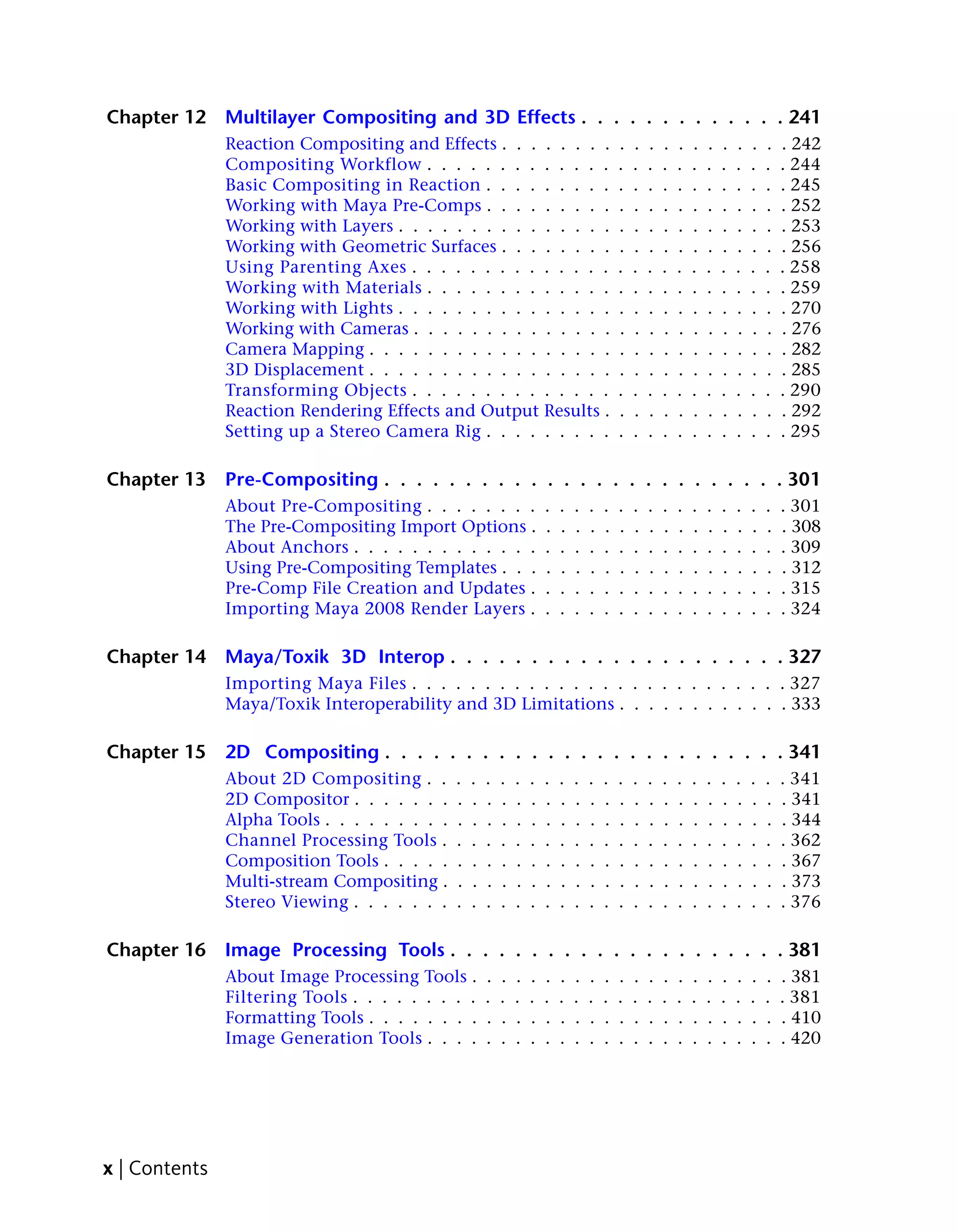


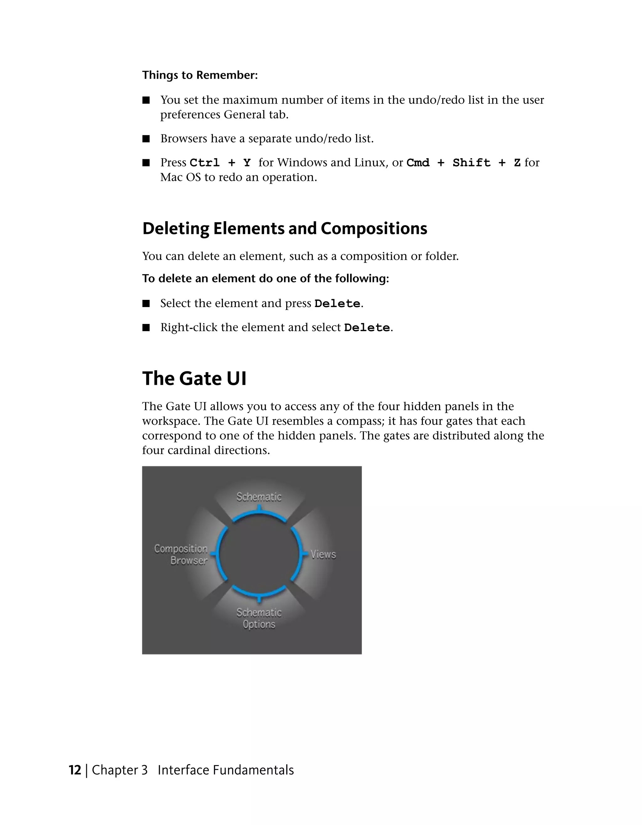

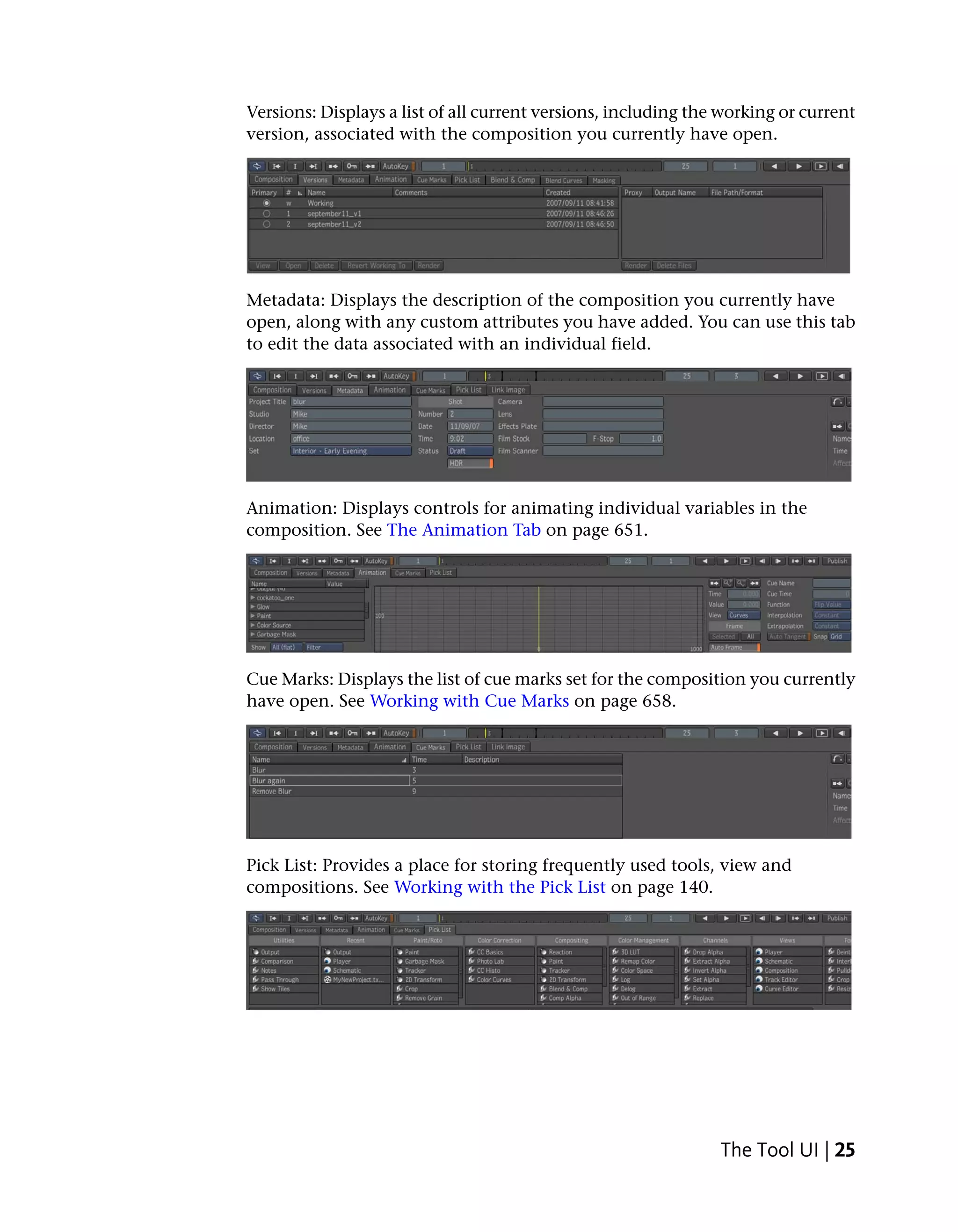
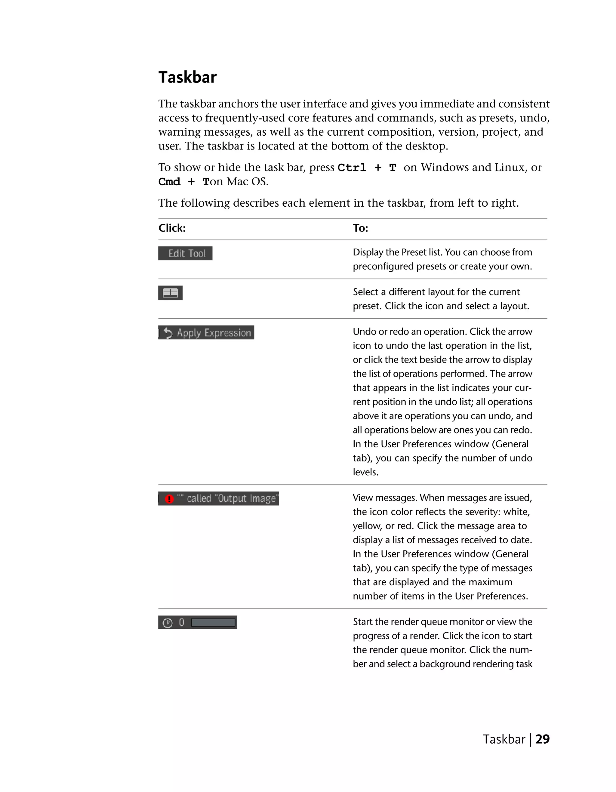
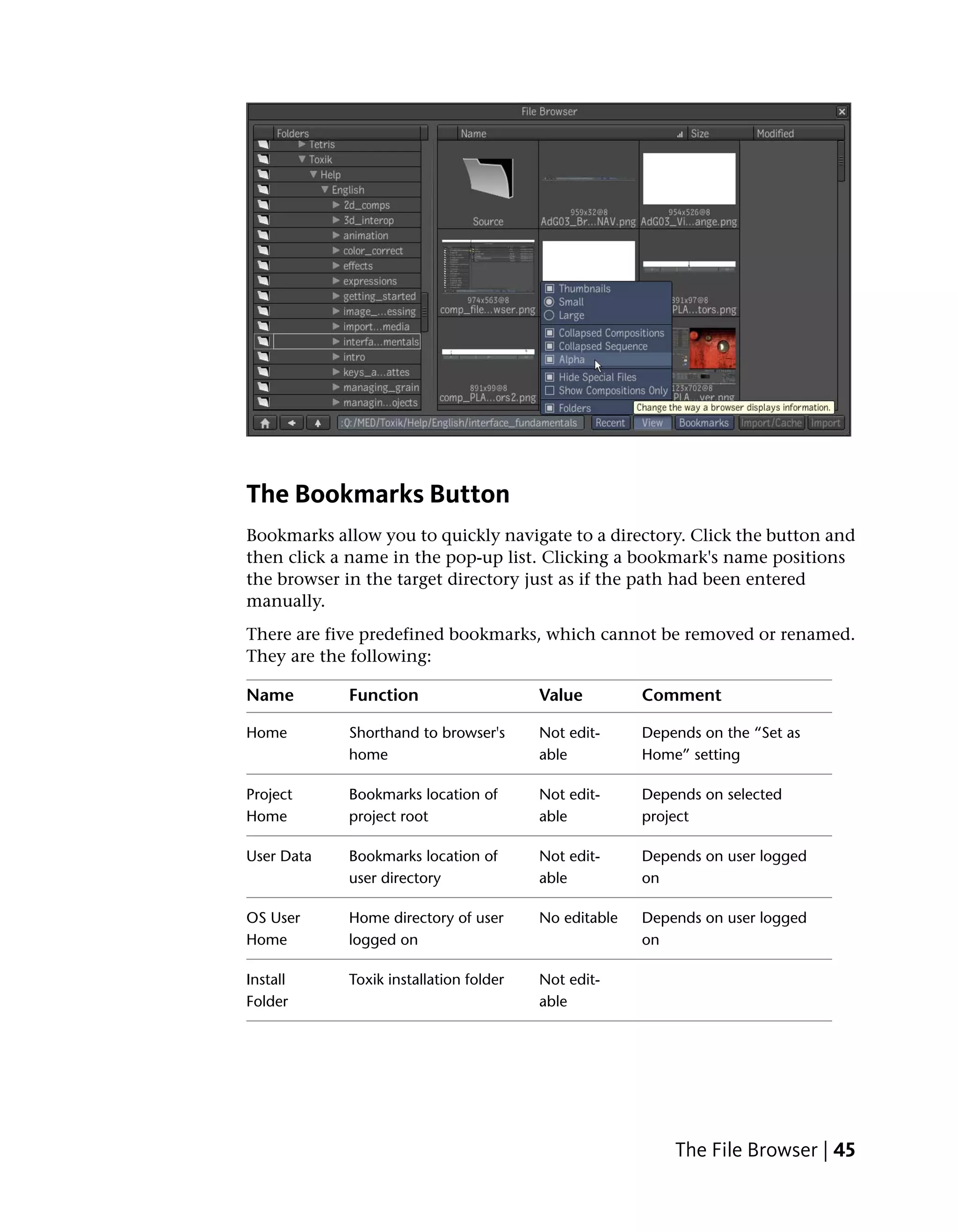
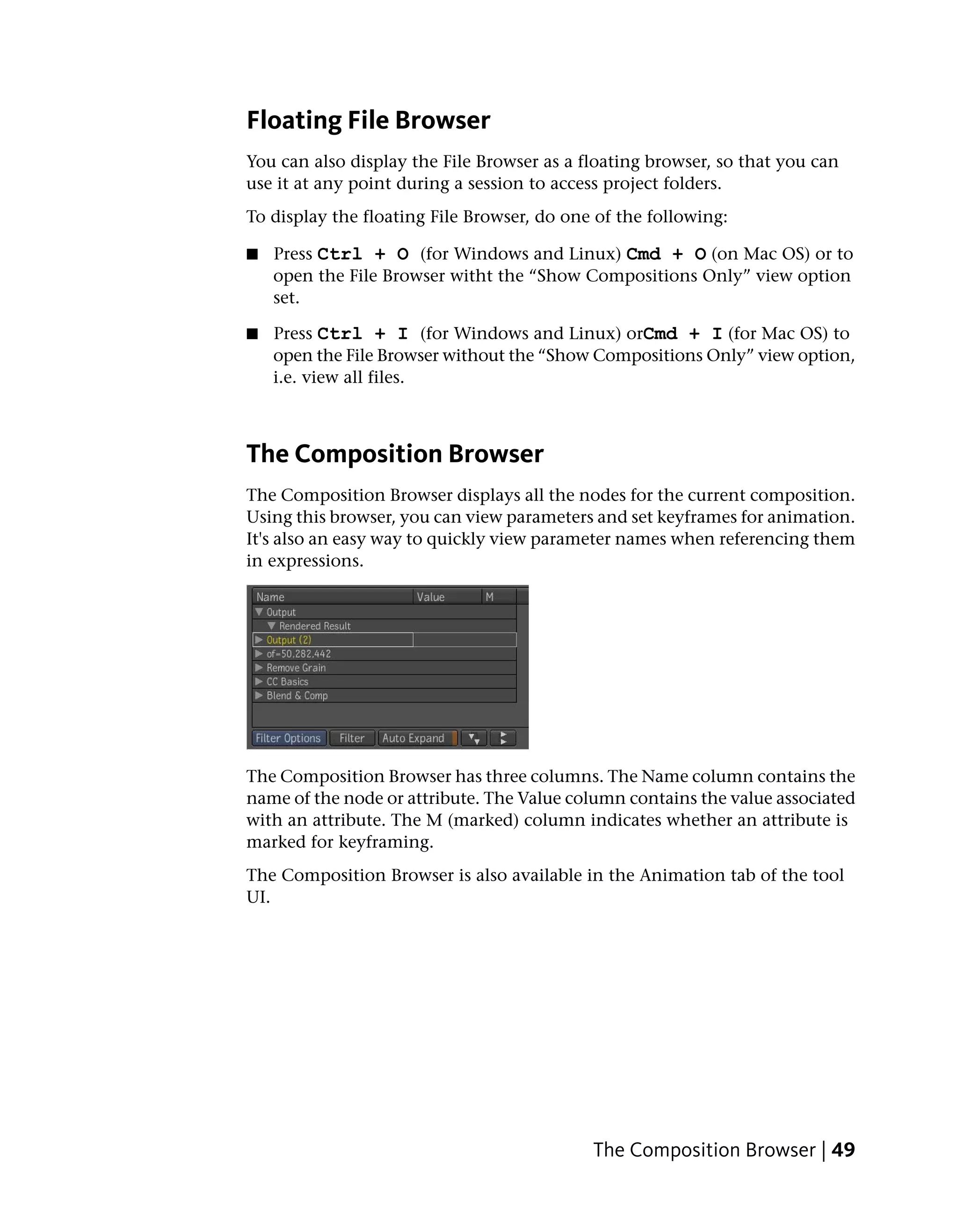
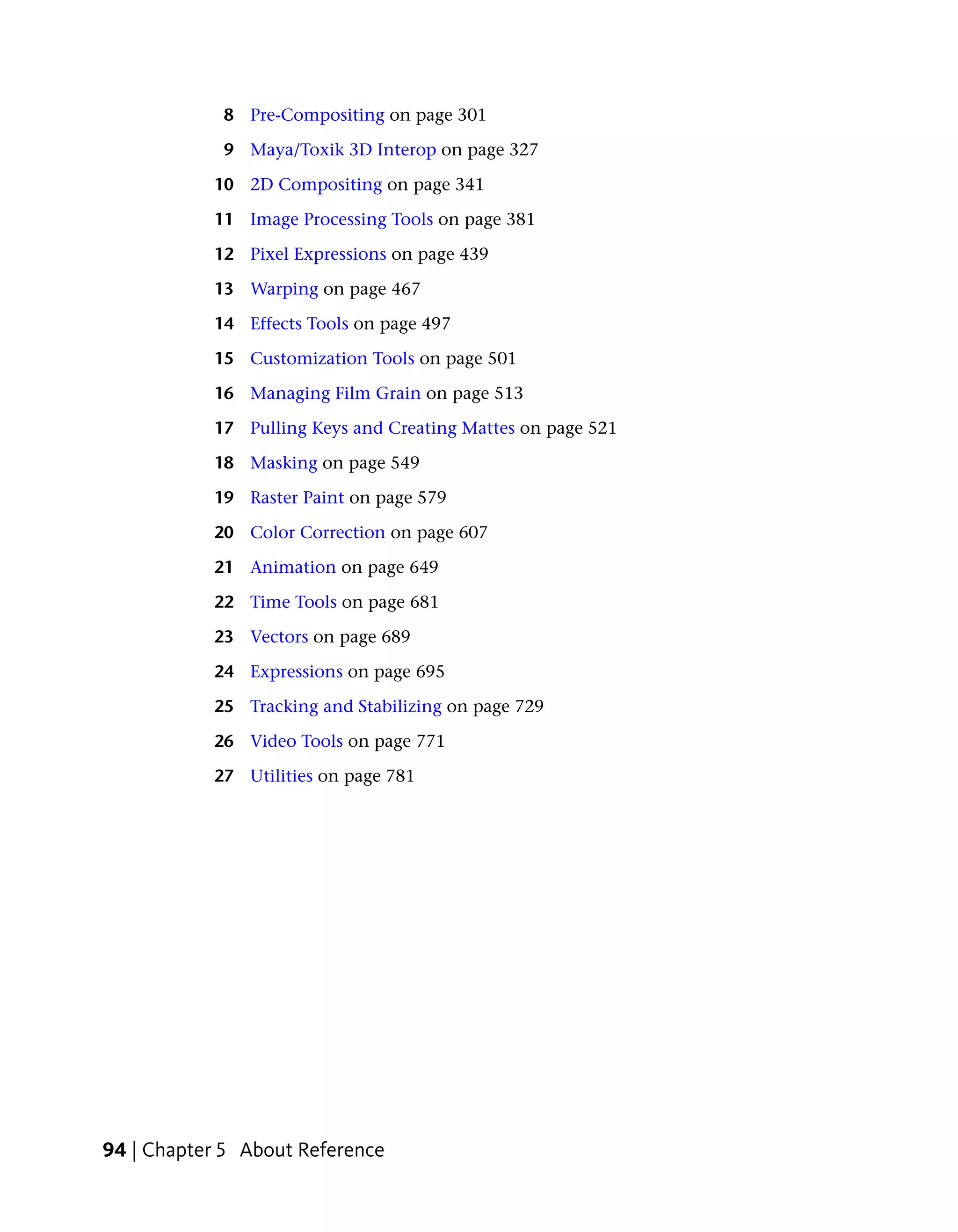
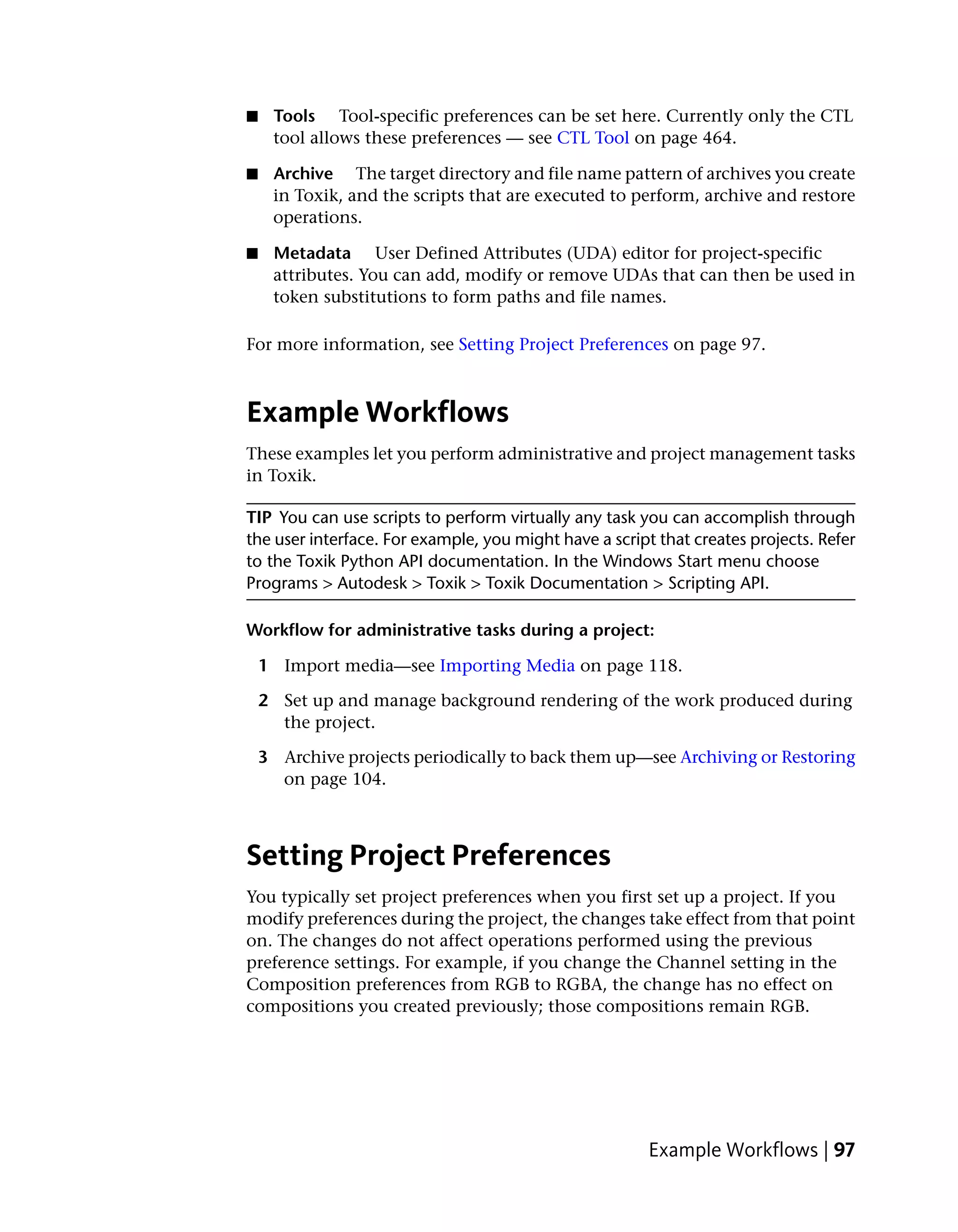


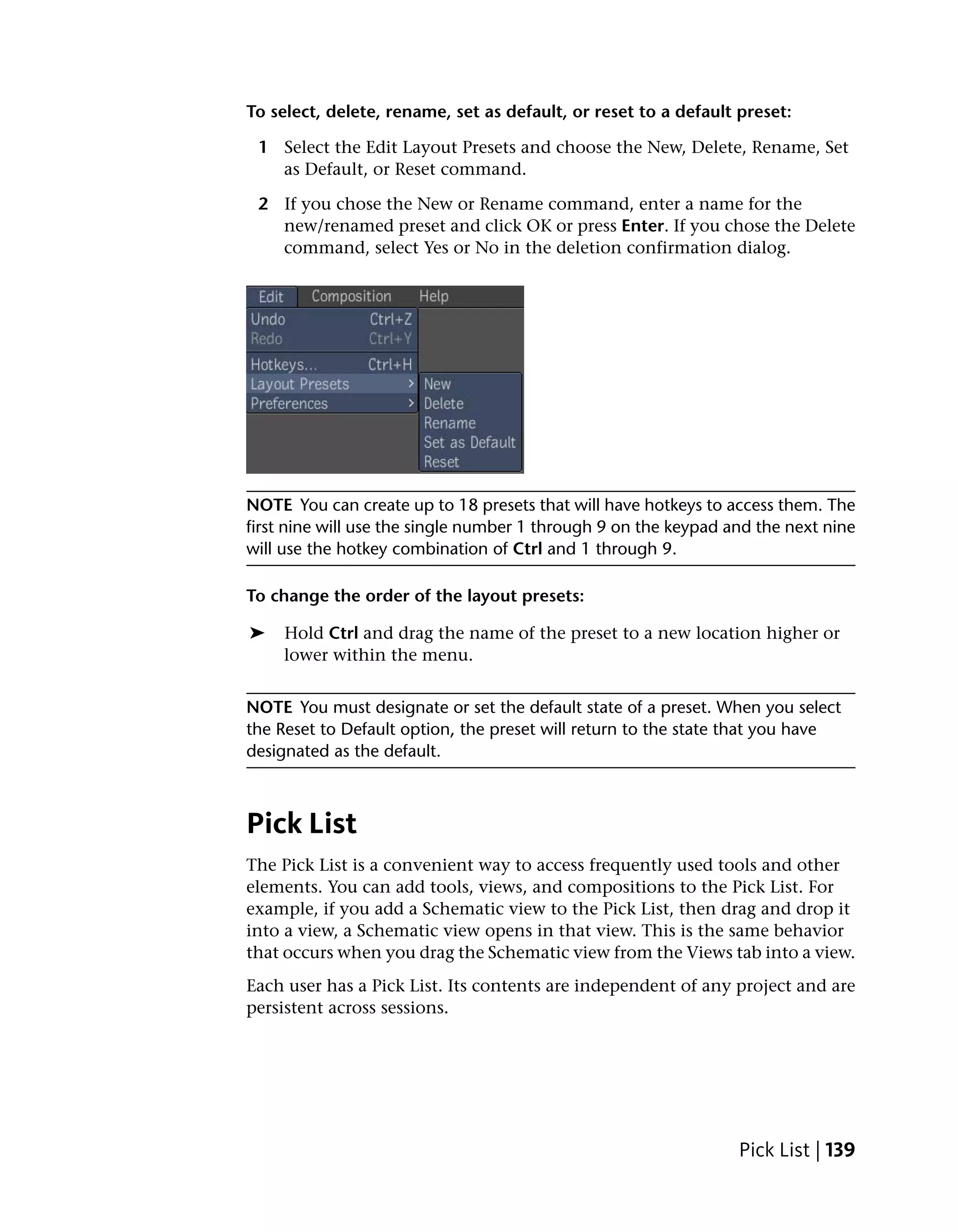

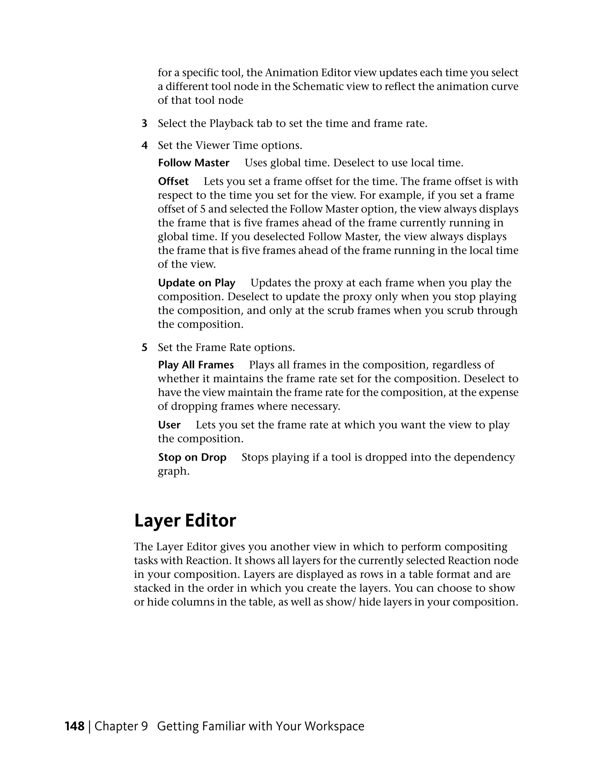
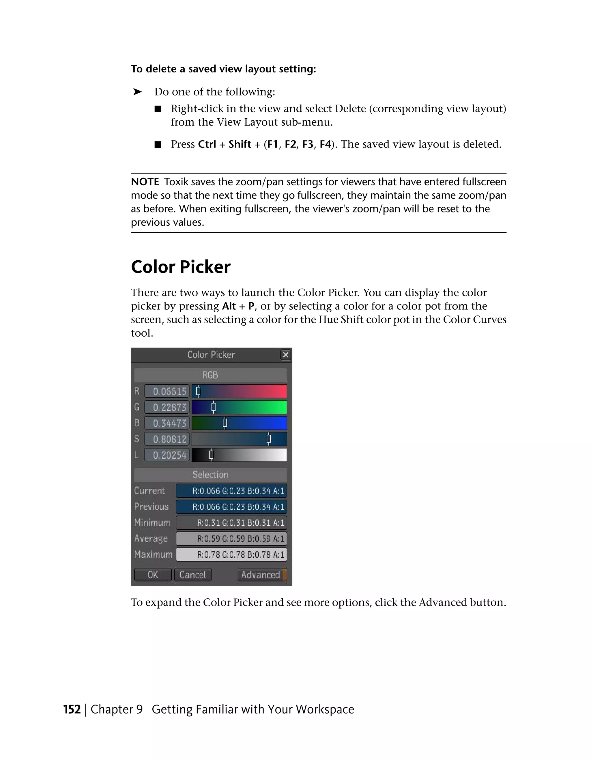
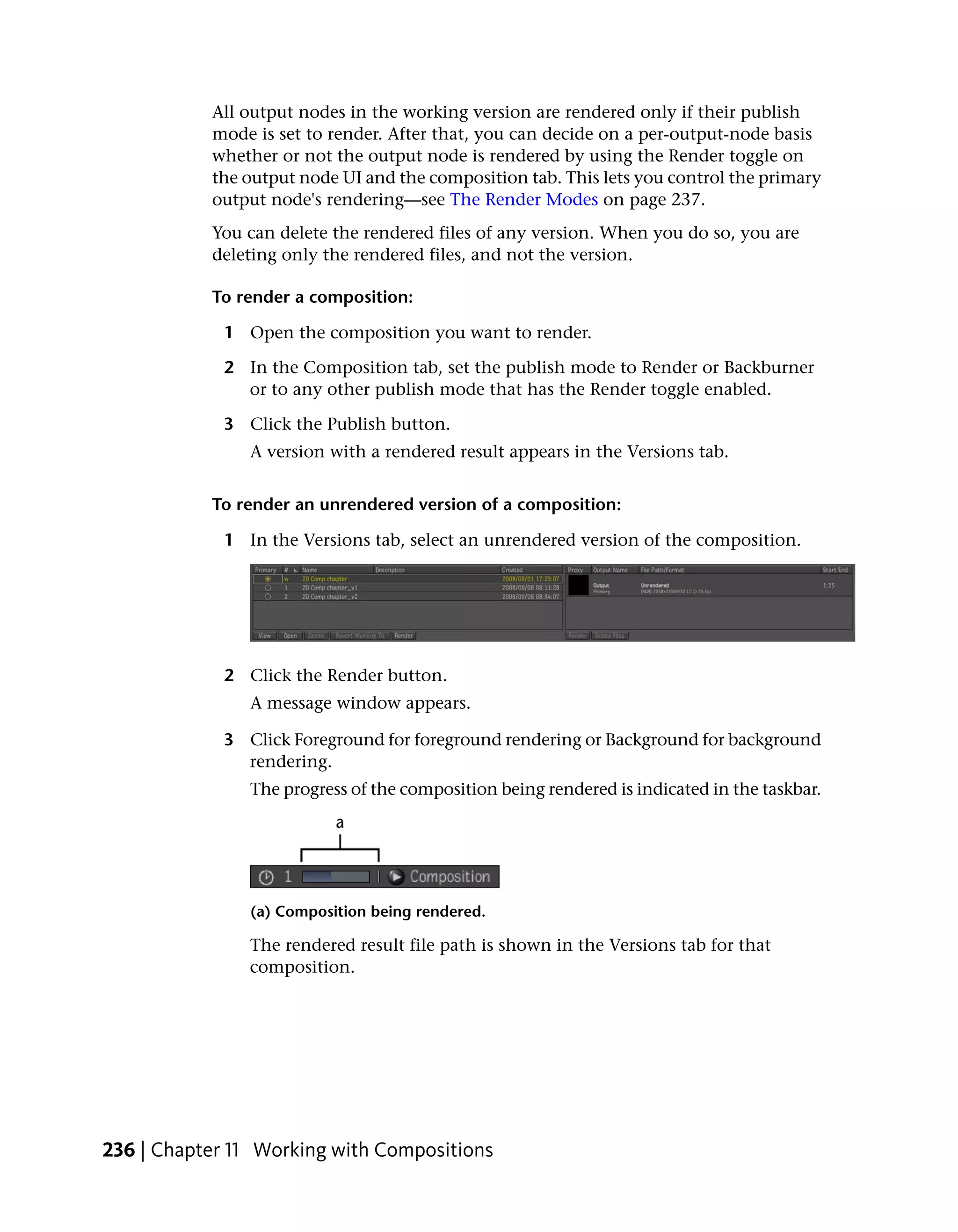
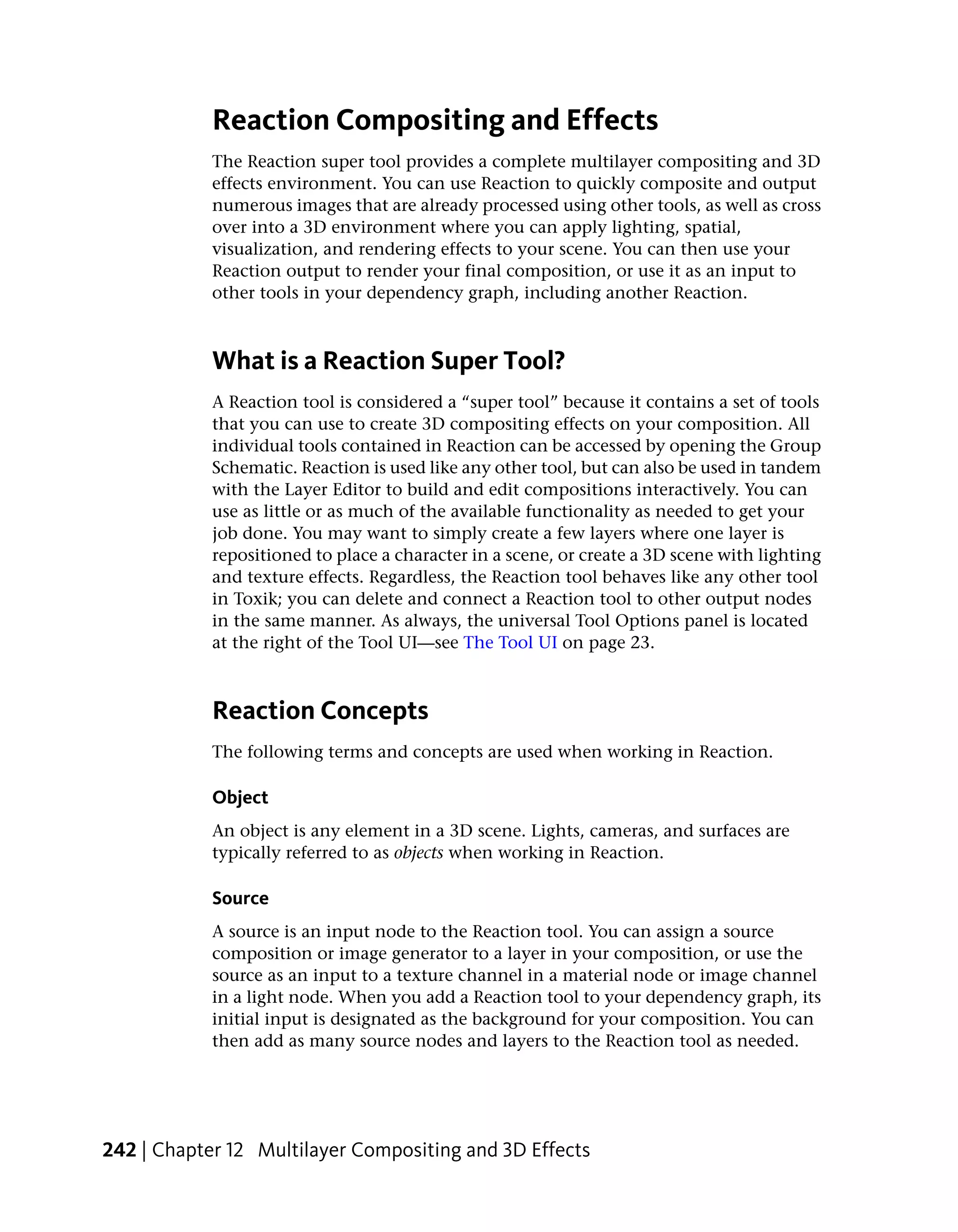
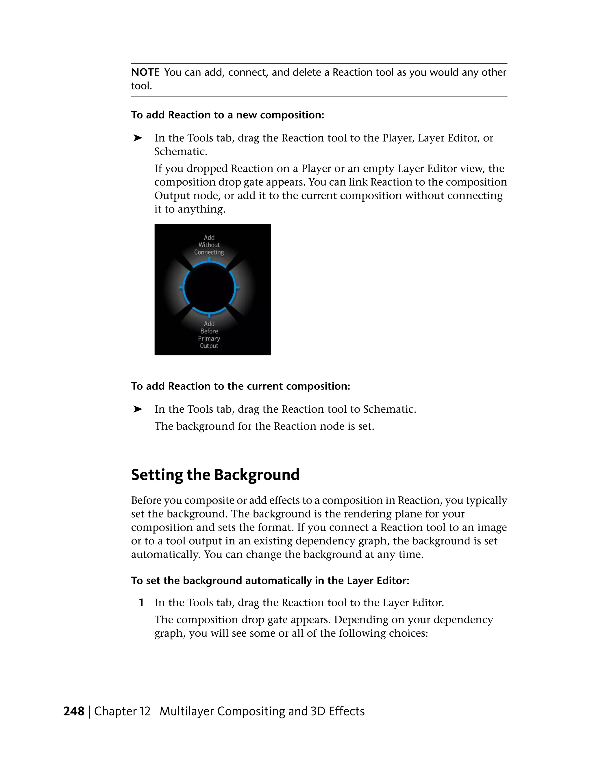
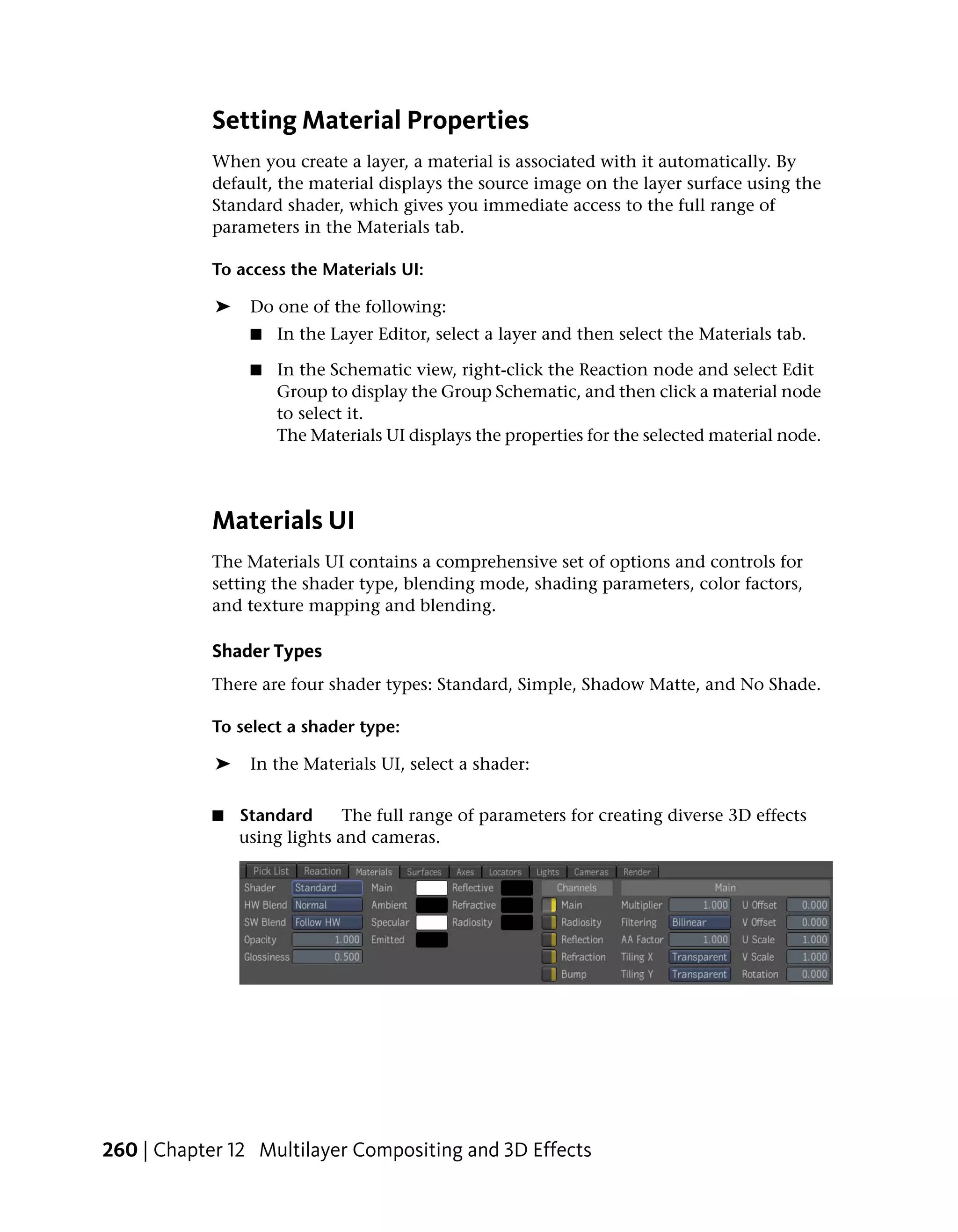
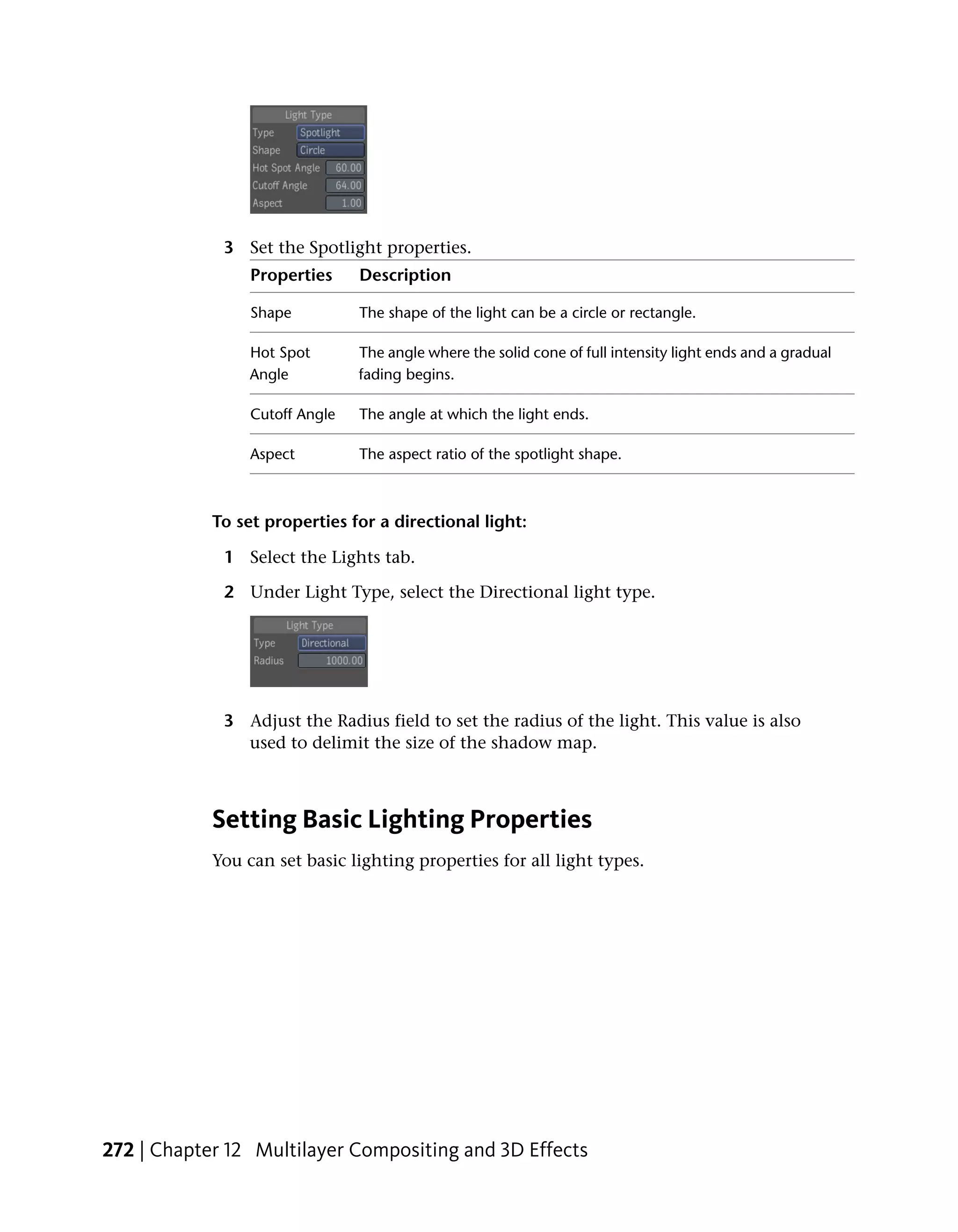
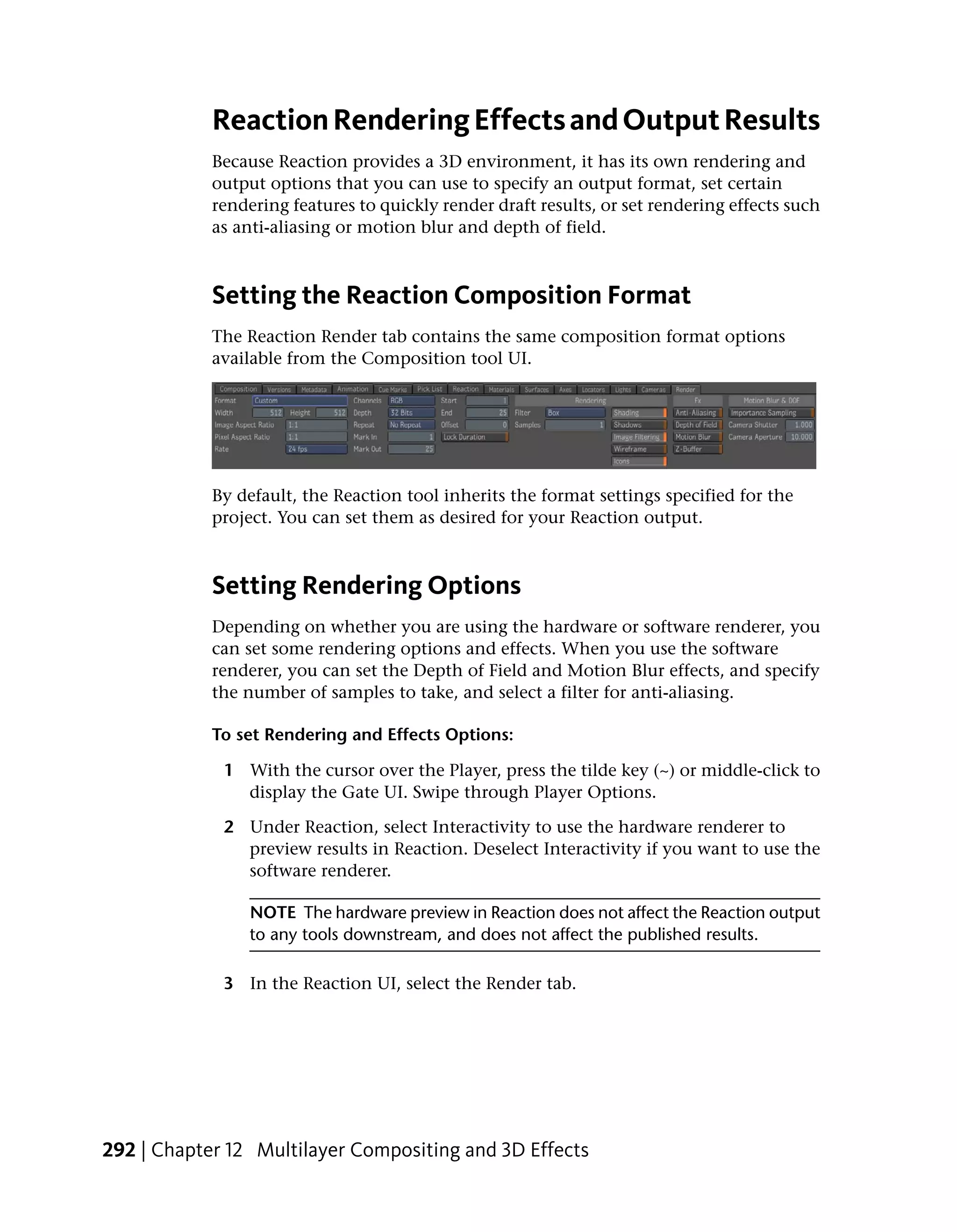

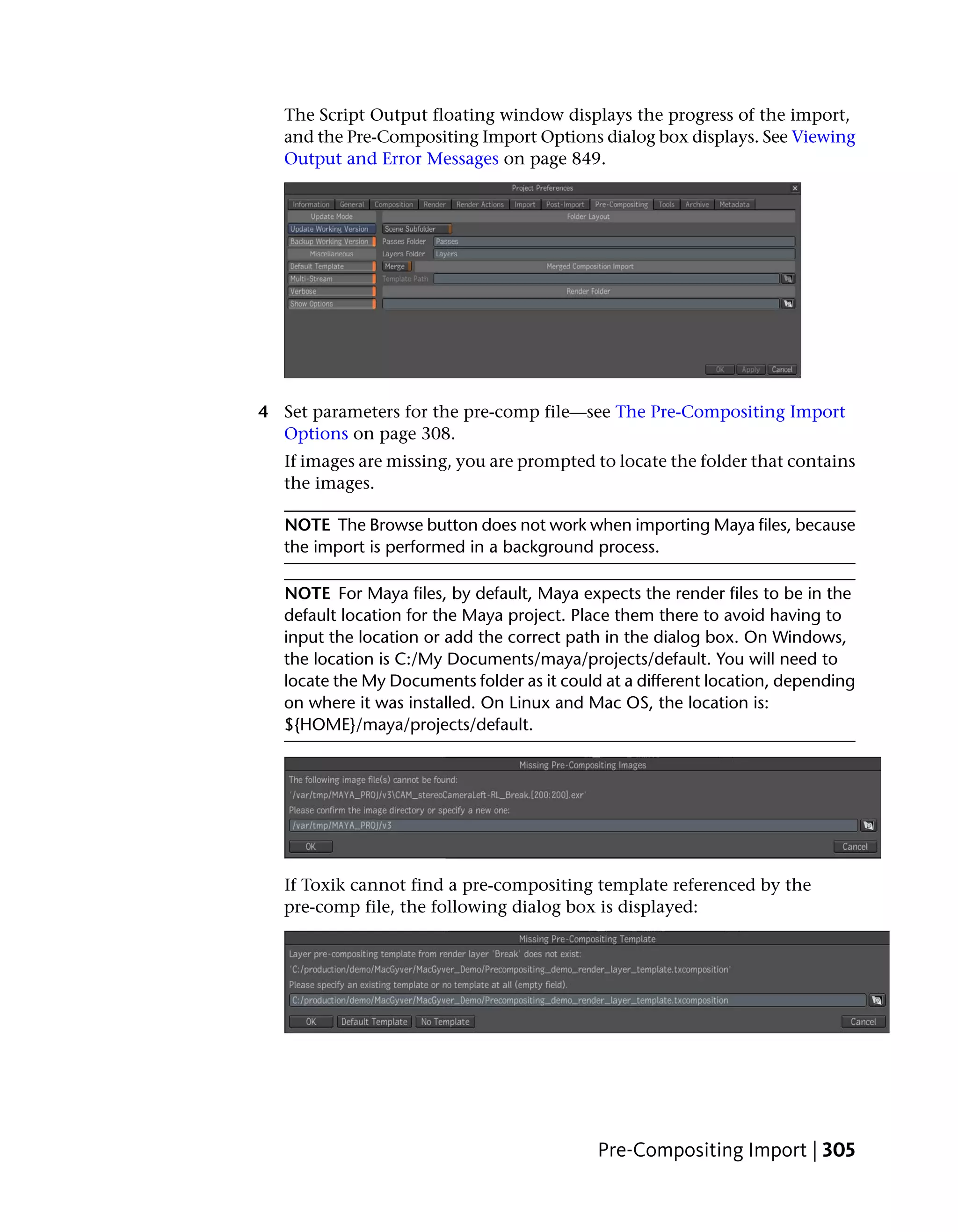
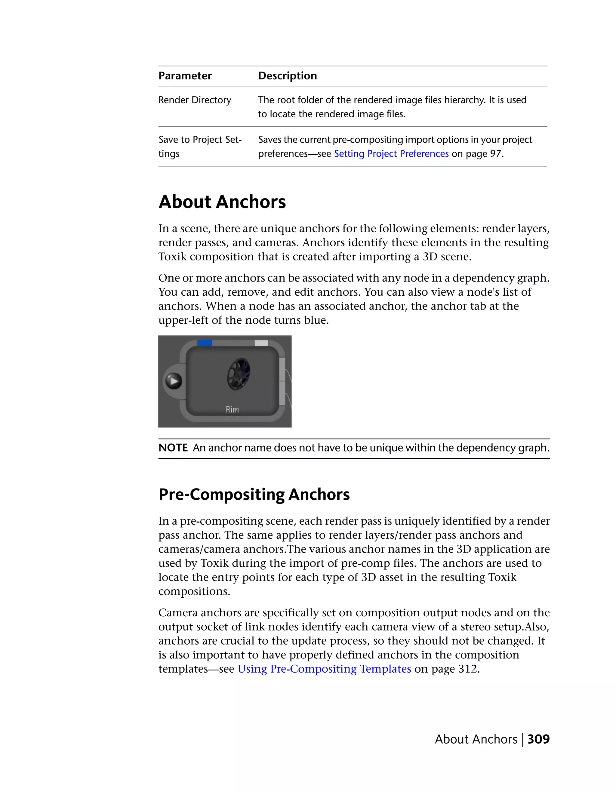
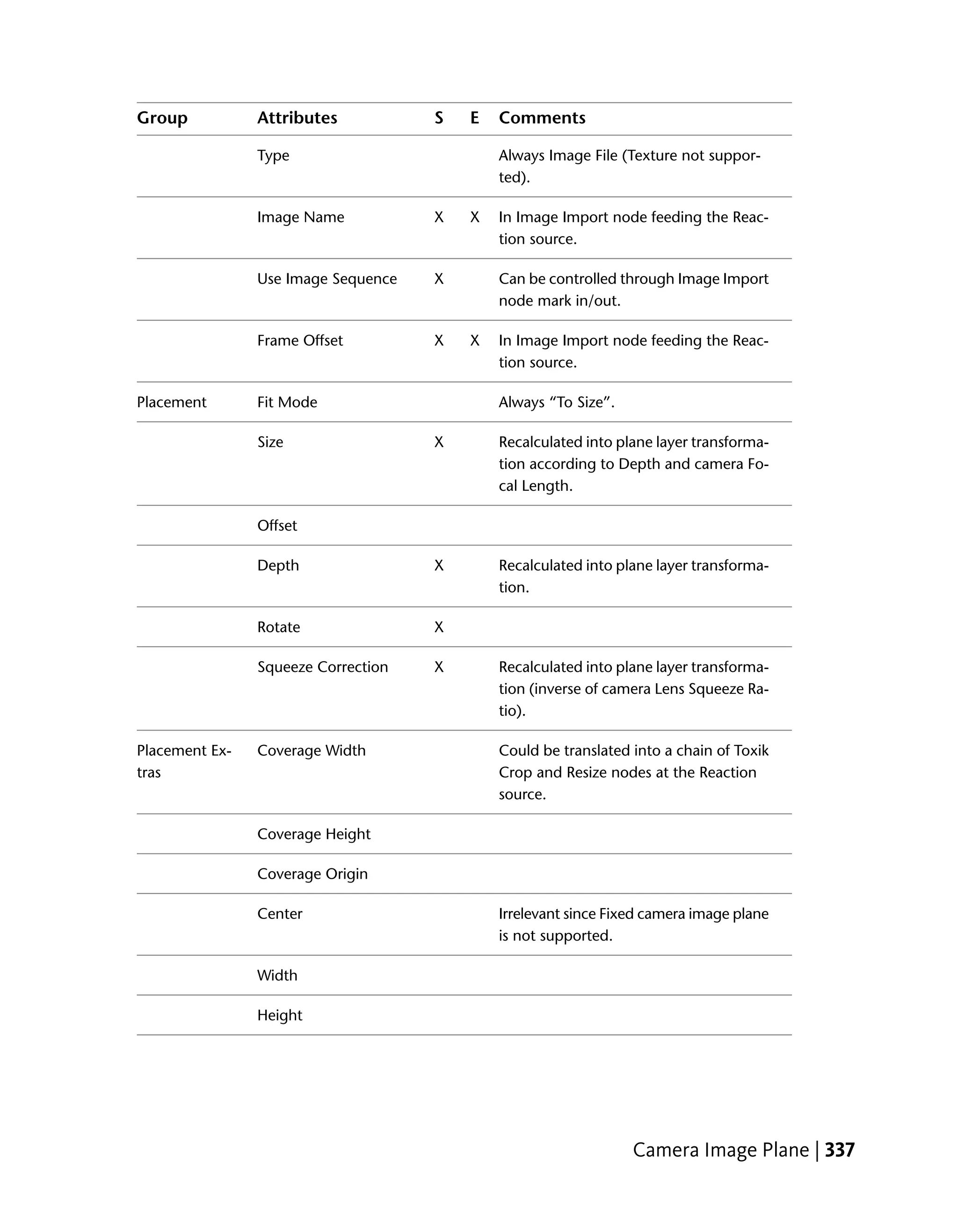

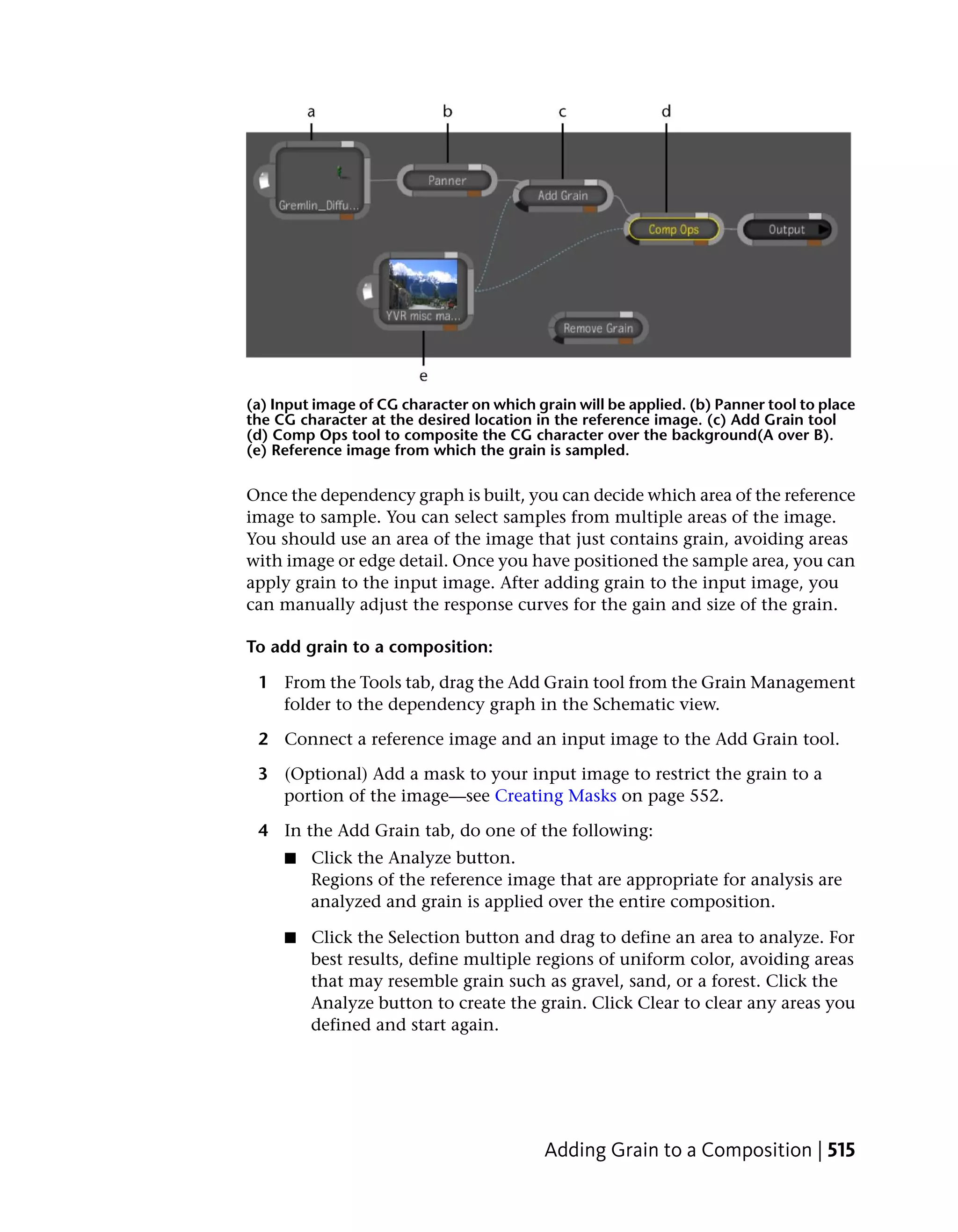
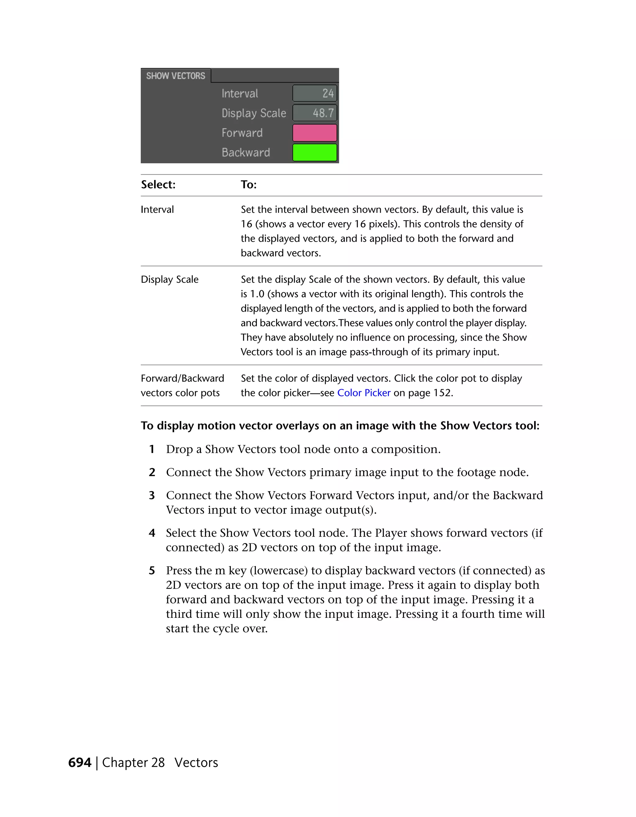
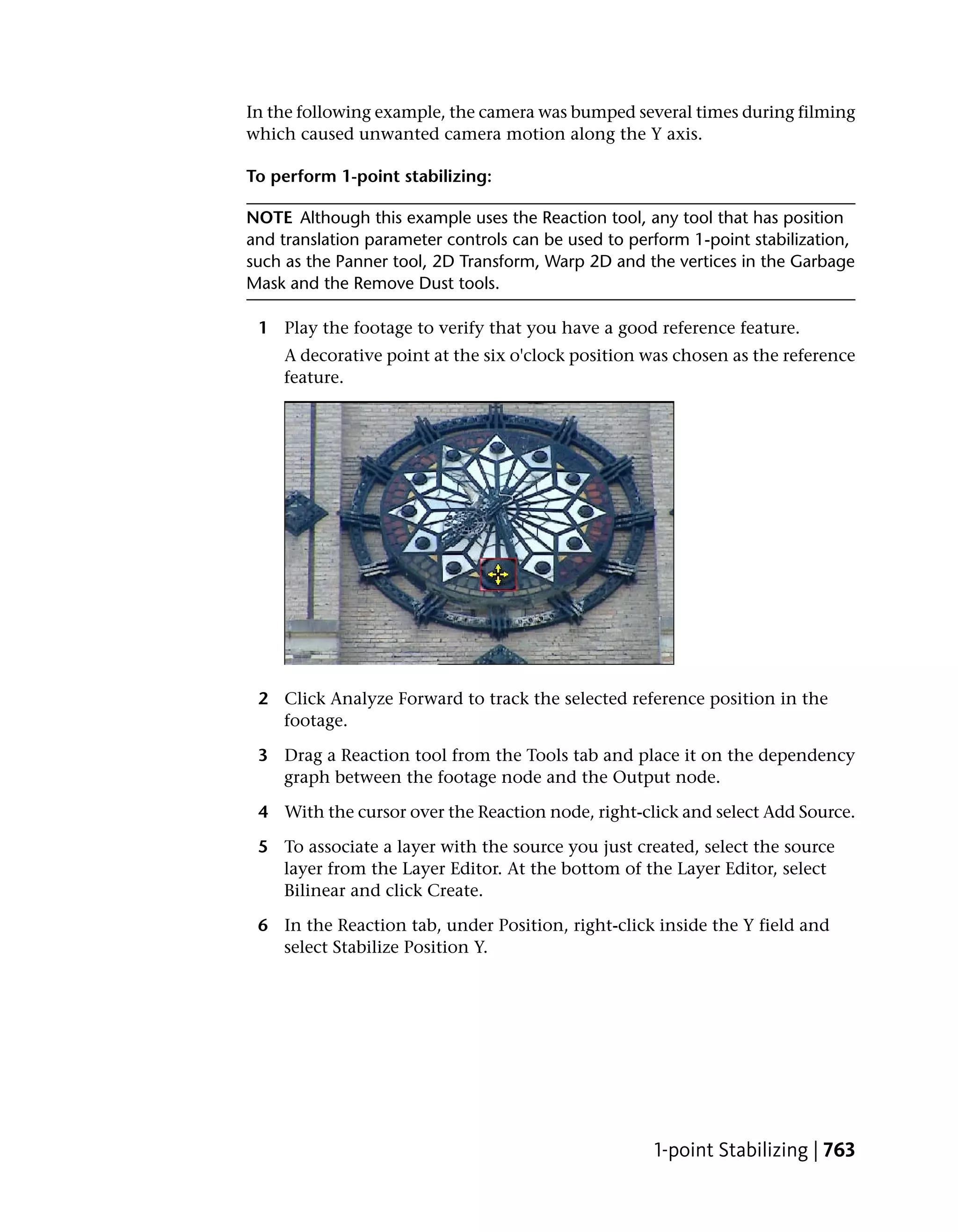
![The Alpha Levels tool UI has the following parameters.
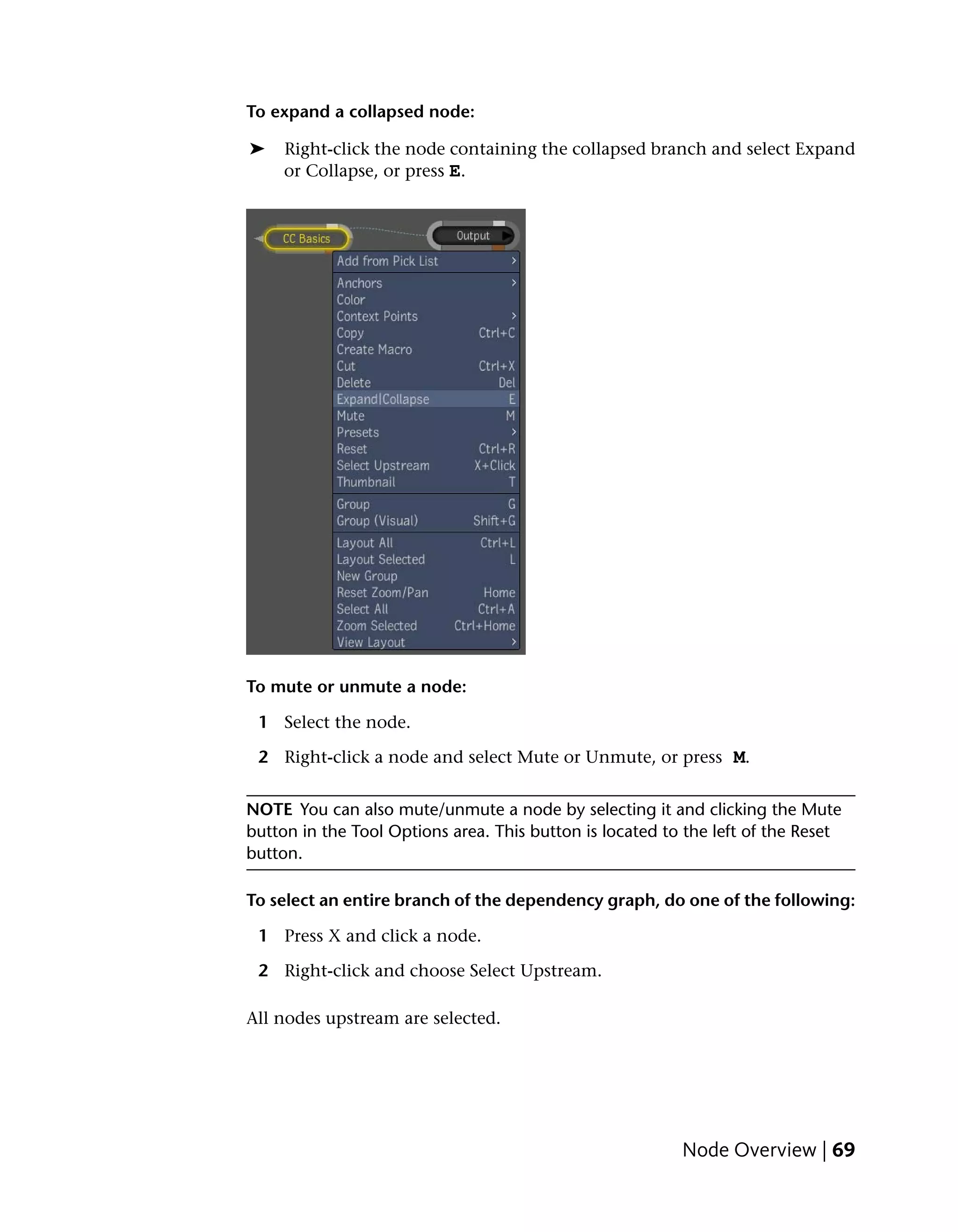
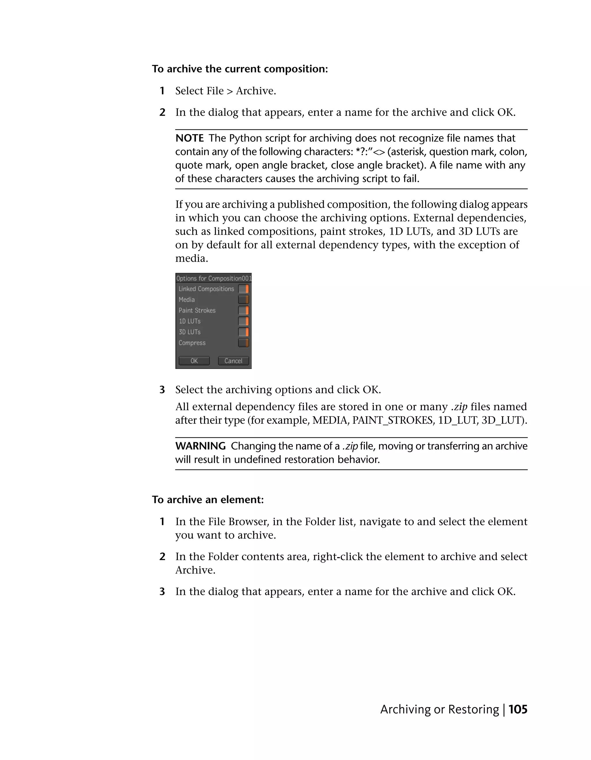
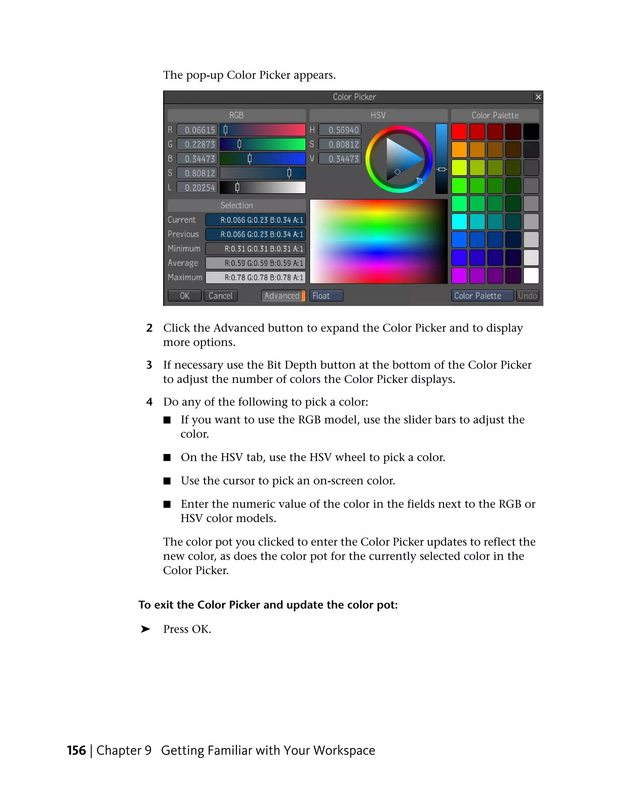
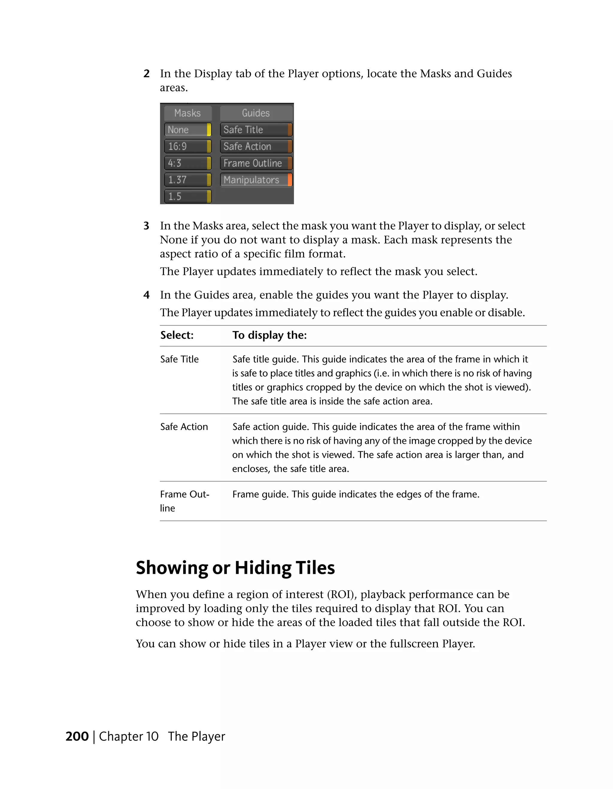
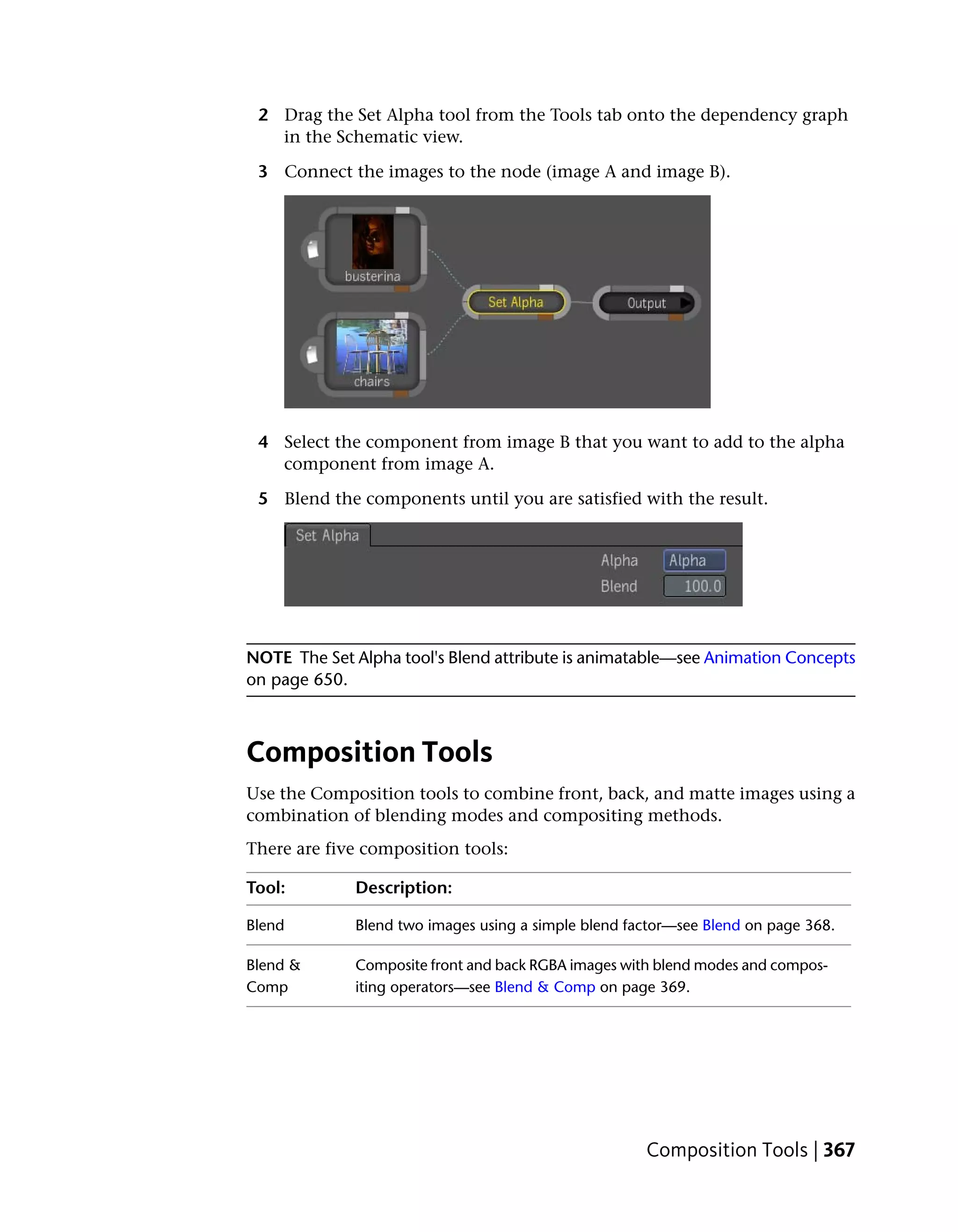
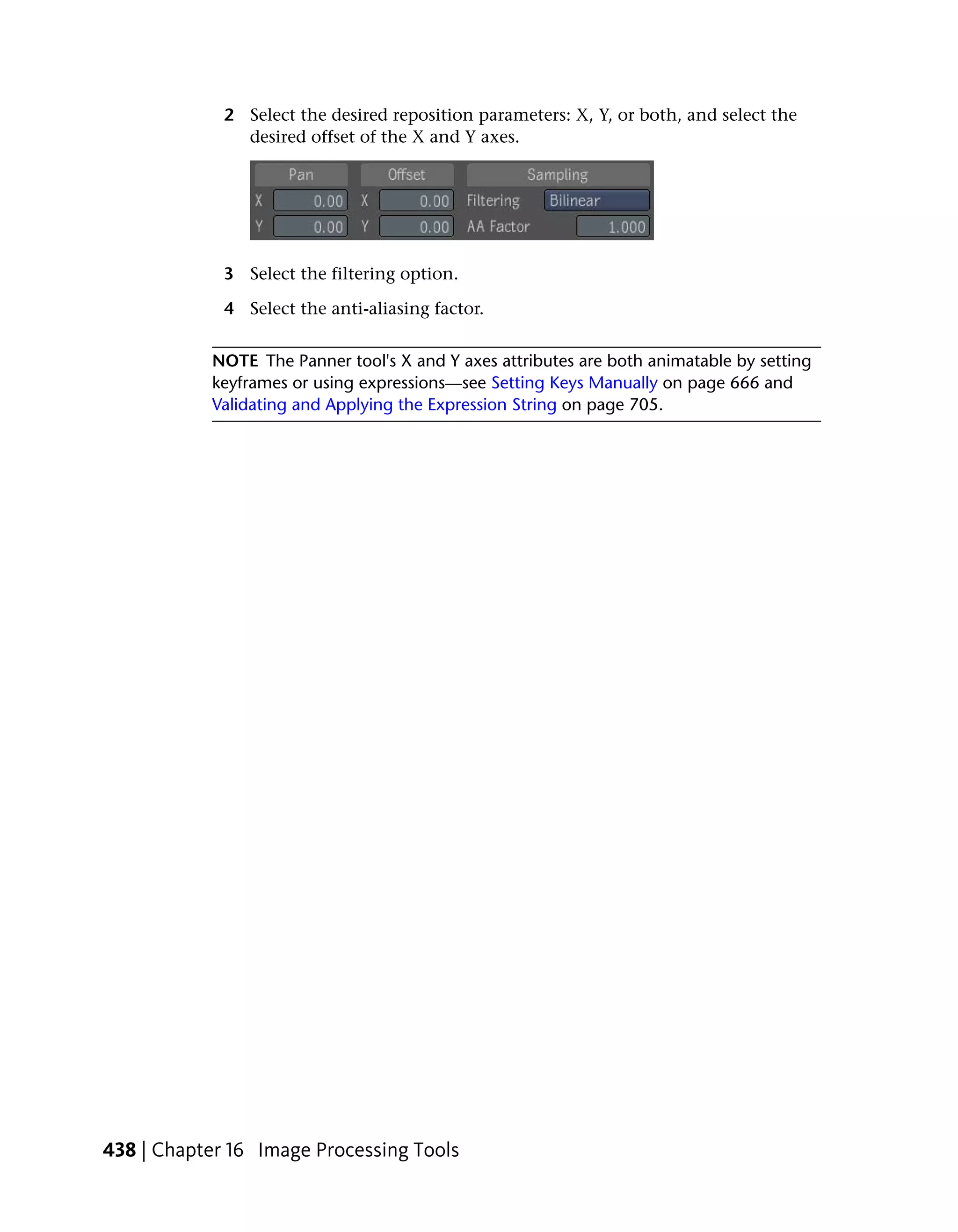
(a) Lift/Gain fields (b) Minimum Output slider and field (c) Minimum Input slider and
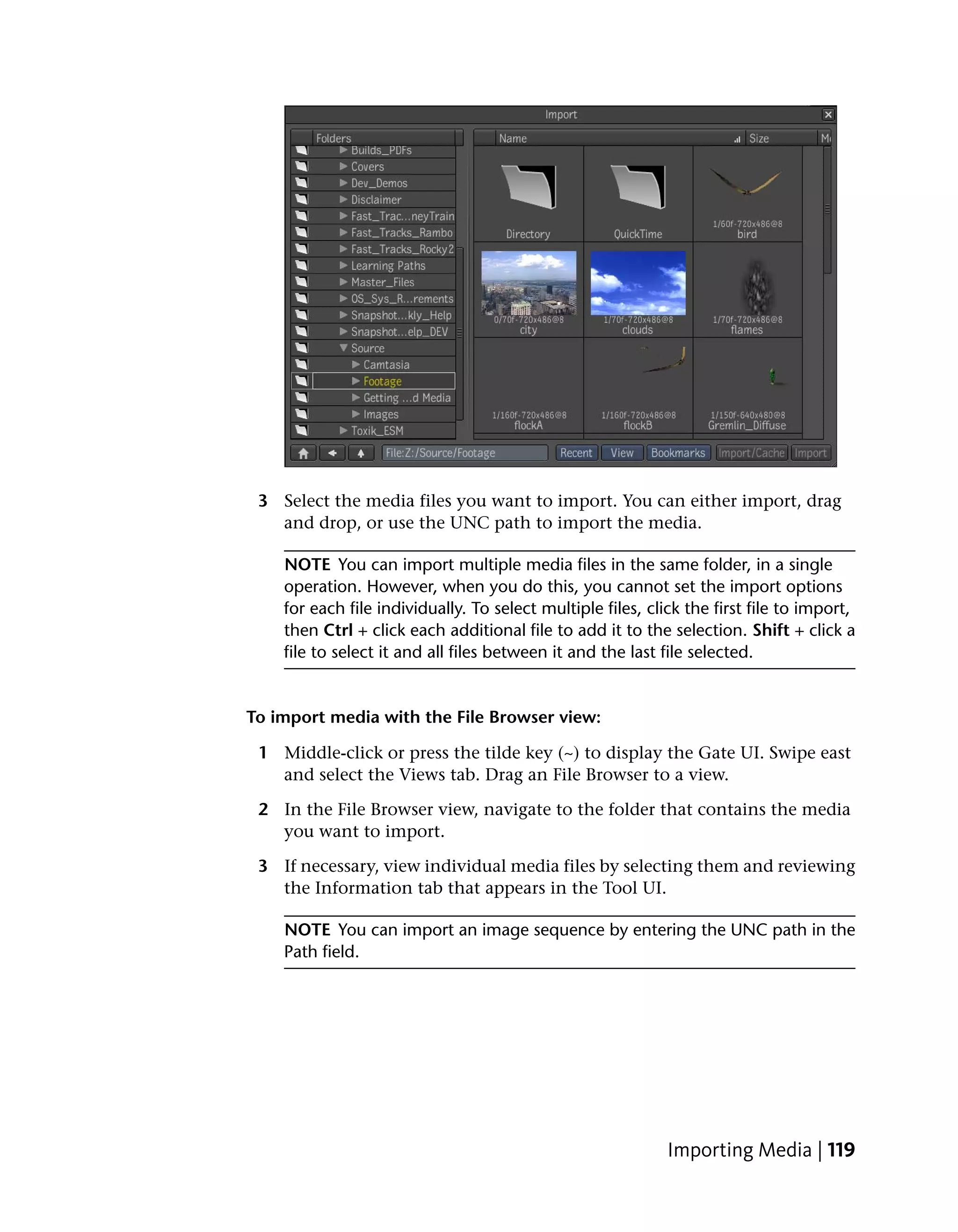
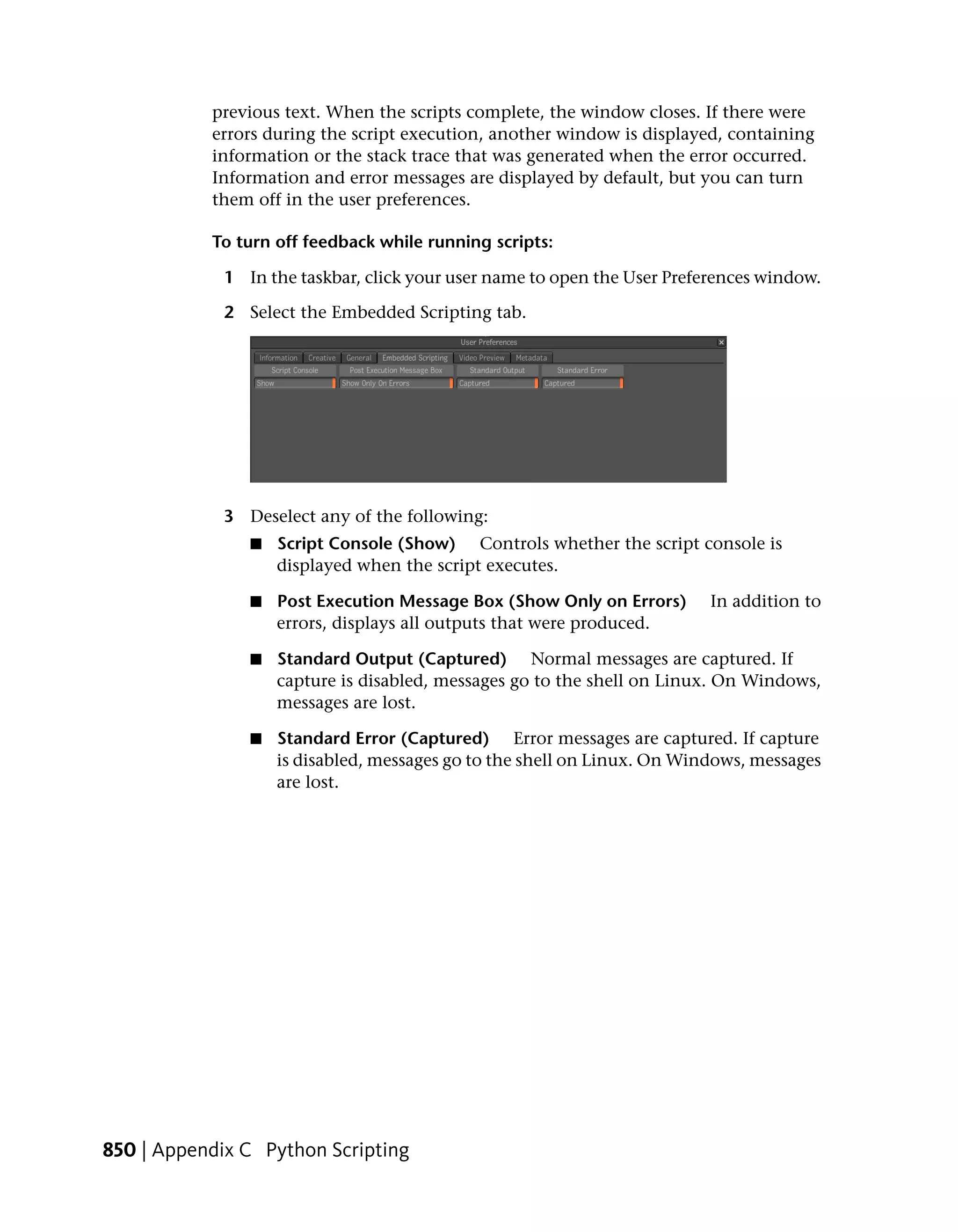
field (d) Luma Remapping Curve (e) Maximum Input slider and field (f) Maximum
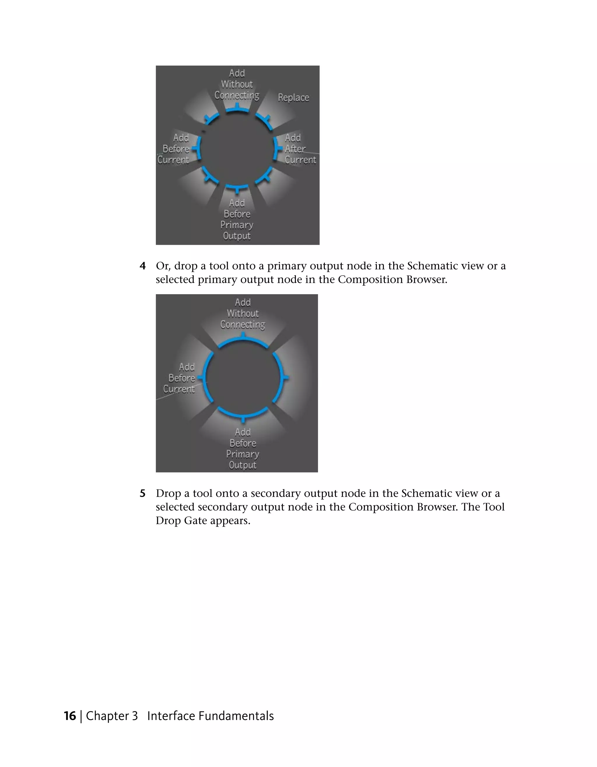
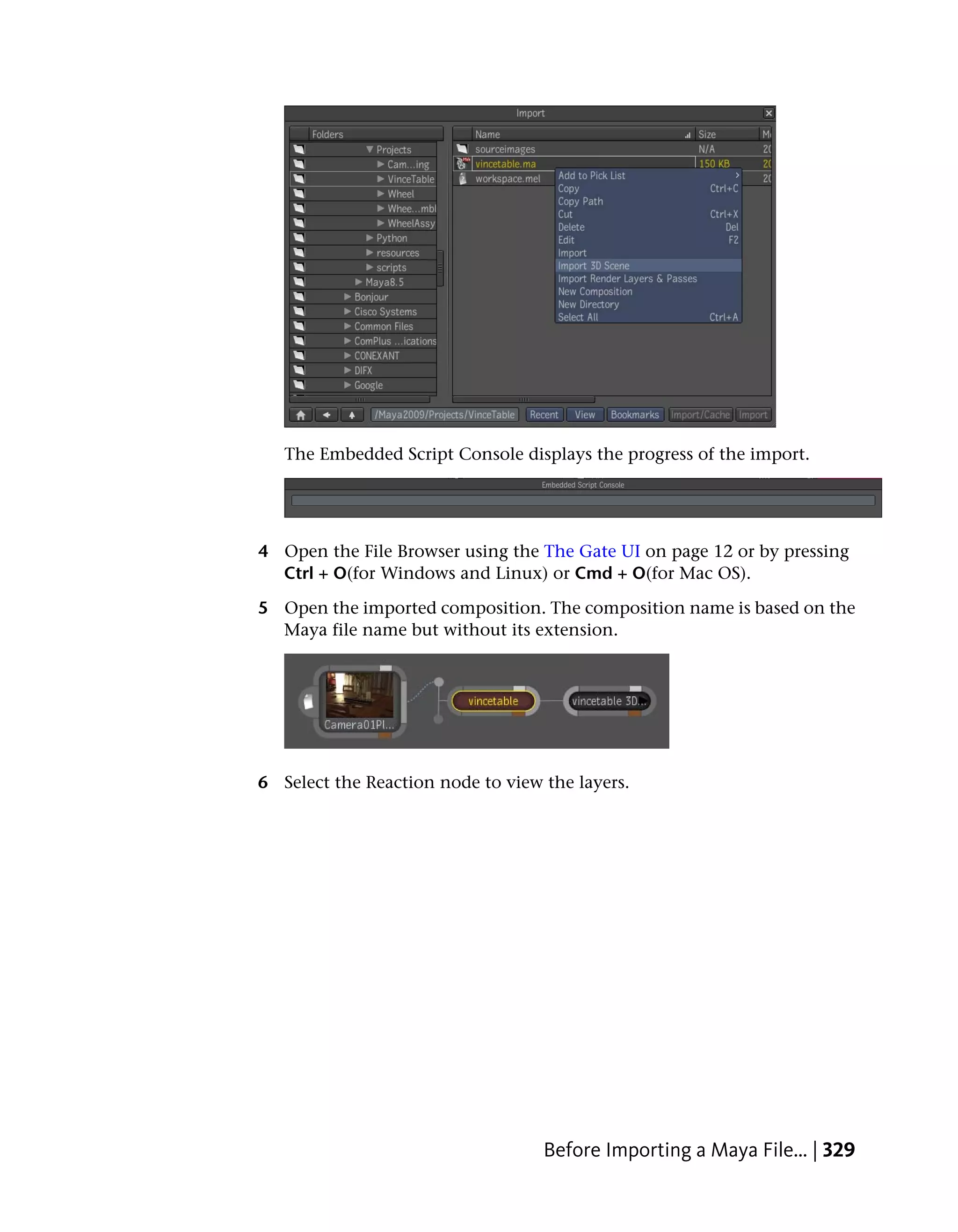
Output slider and field
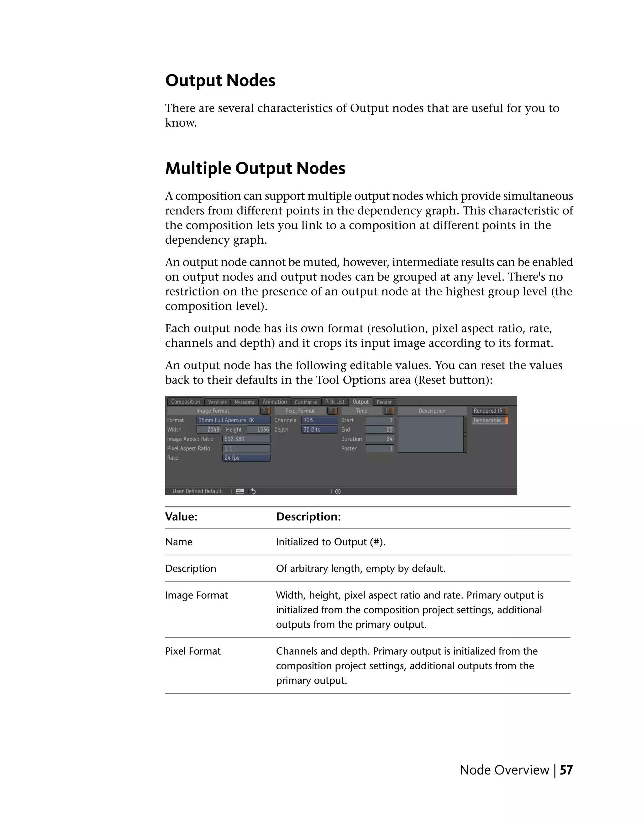
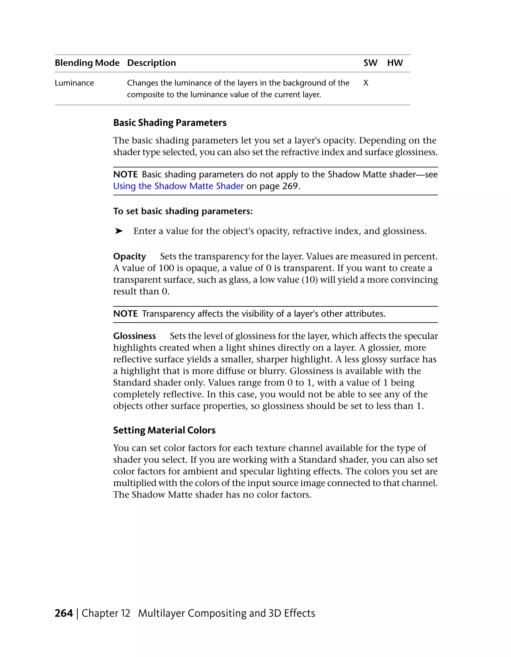
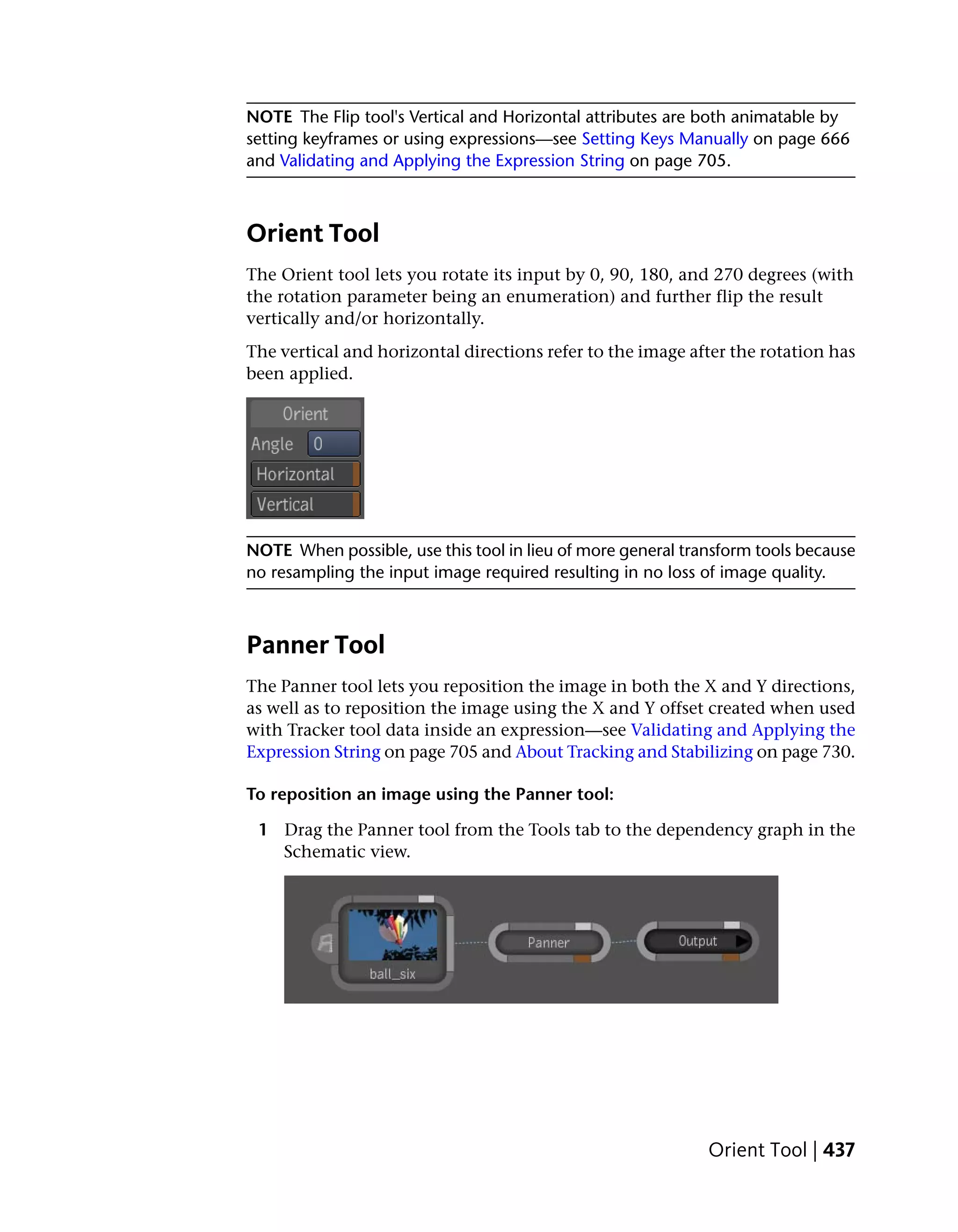
■ Lift Adjust the Lift to add an overall offset to the matte.
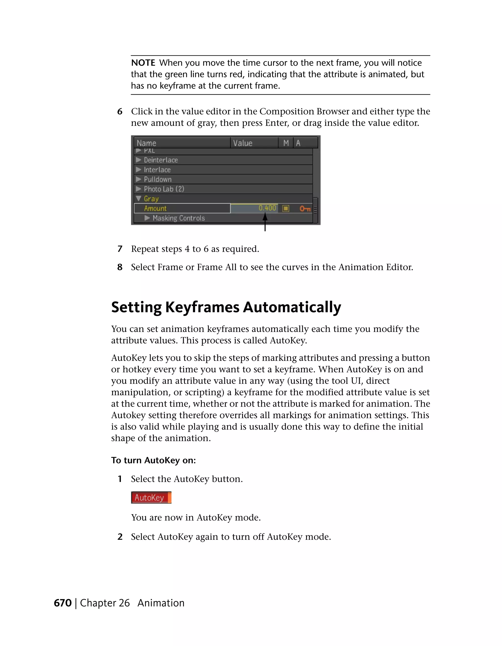
■ Gain Adjust the Gain to adjust a scaling factor for the matte. Lift, Gain,
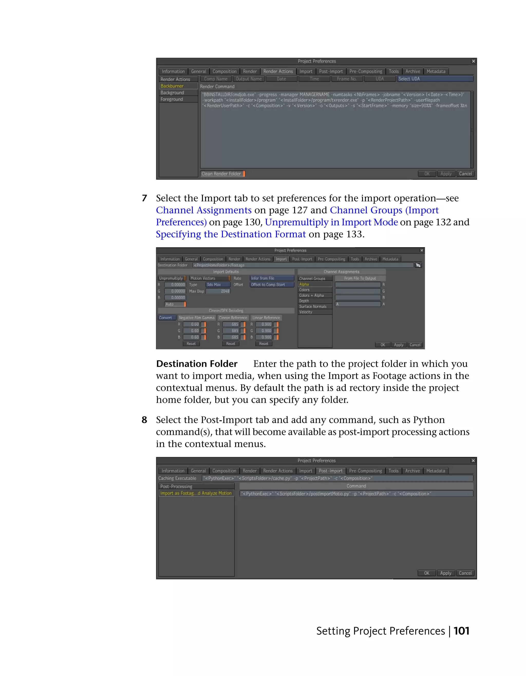
Input and Output are animatable attributes—see Marking Attributes for
Keyframing on page 664.
■ Minimum Output slider Drag to remap input blacks to dark gray.
■ Minimum Input slider Drag to the right to remap dark grays as black.
■ Luma remapping curve View the changes you make in this curve.
■ Maximum Input slider Drag to the left to remap light grays as white.
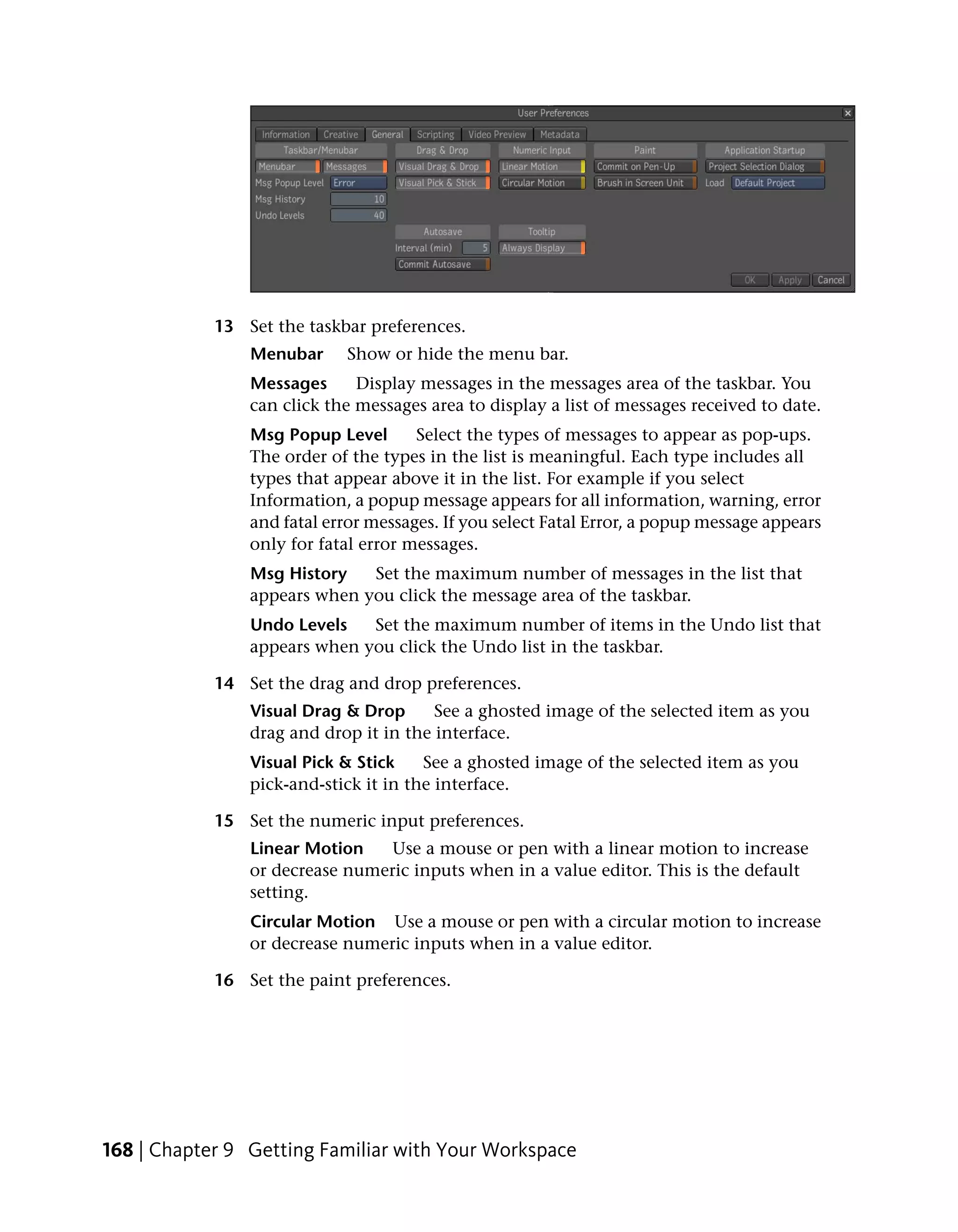
■ Maximum Output slider Drag to the left to remap output whites to light
gray.
Blend Alpha
The Blend Alpha tool is used to blend two mattes together under the optional
control of a third matte. It has front, back, and matte inputs. It extracts a
matte from the front image and composites it over the alpha channel of the
back input using a choice of blend modes. The coverage of the front can be
controlled by the matte input. The back is the primary input; the output
inherits the format of the back input; this tool only affects alpha; if the back
is an RGBA image, the color part is simply copied to the output.
NOTE The alpha output of this tool is always clamped to the [0,1] interval.
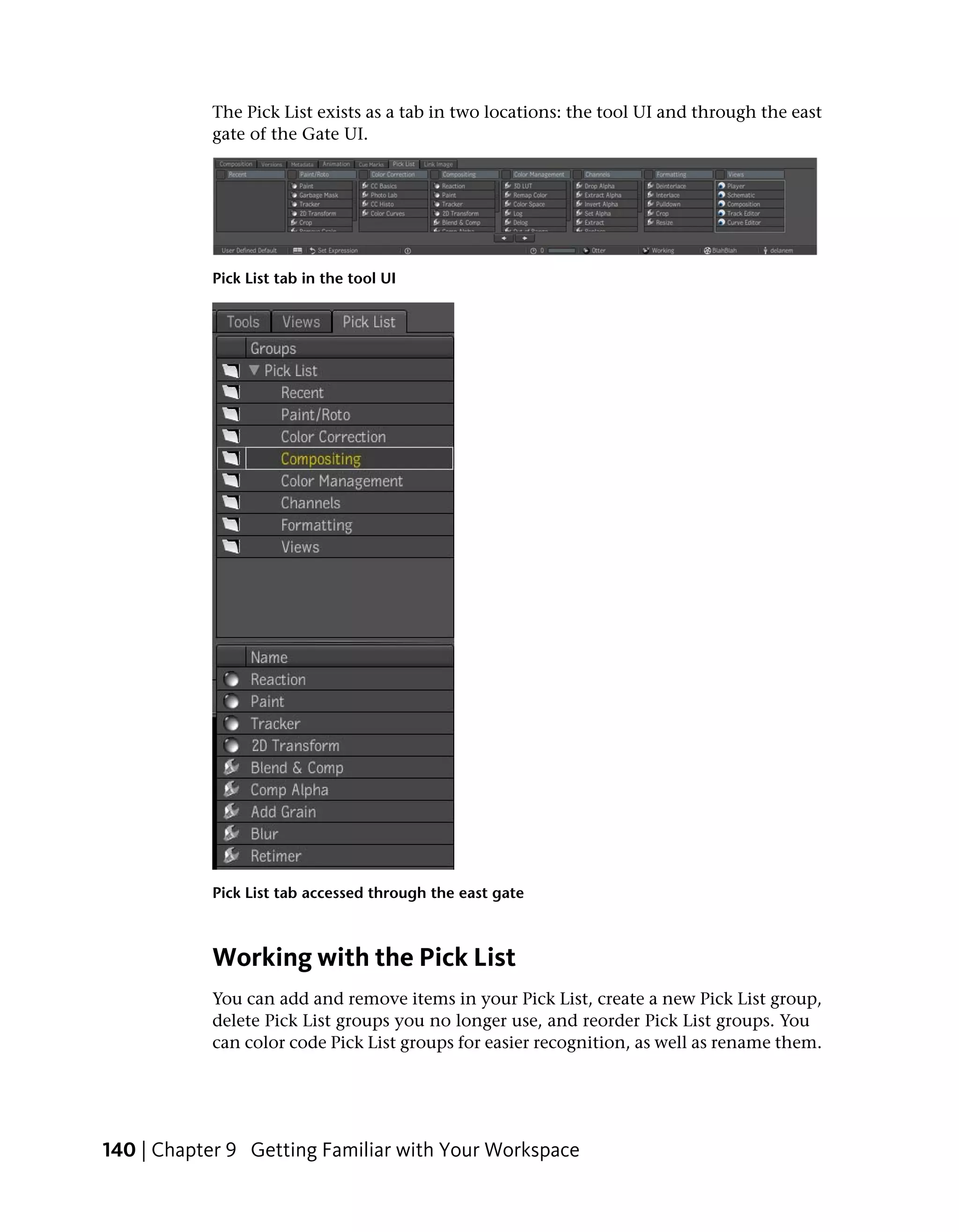
The Blend Alpha tool has the following parameters:
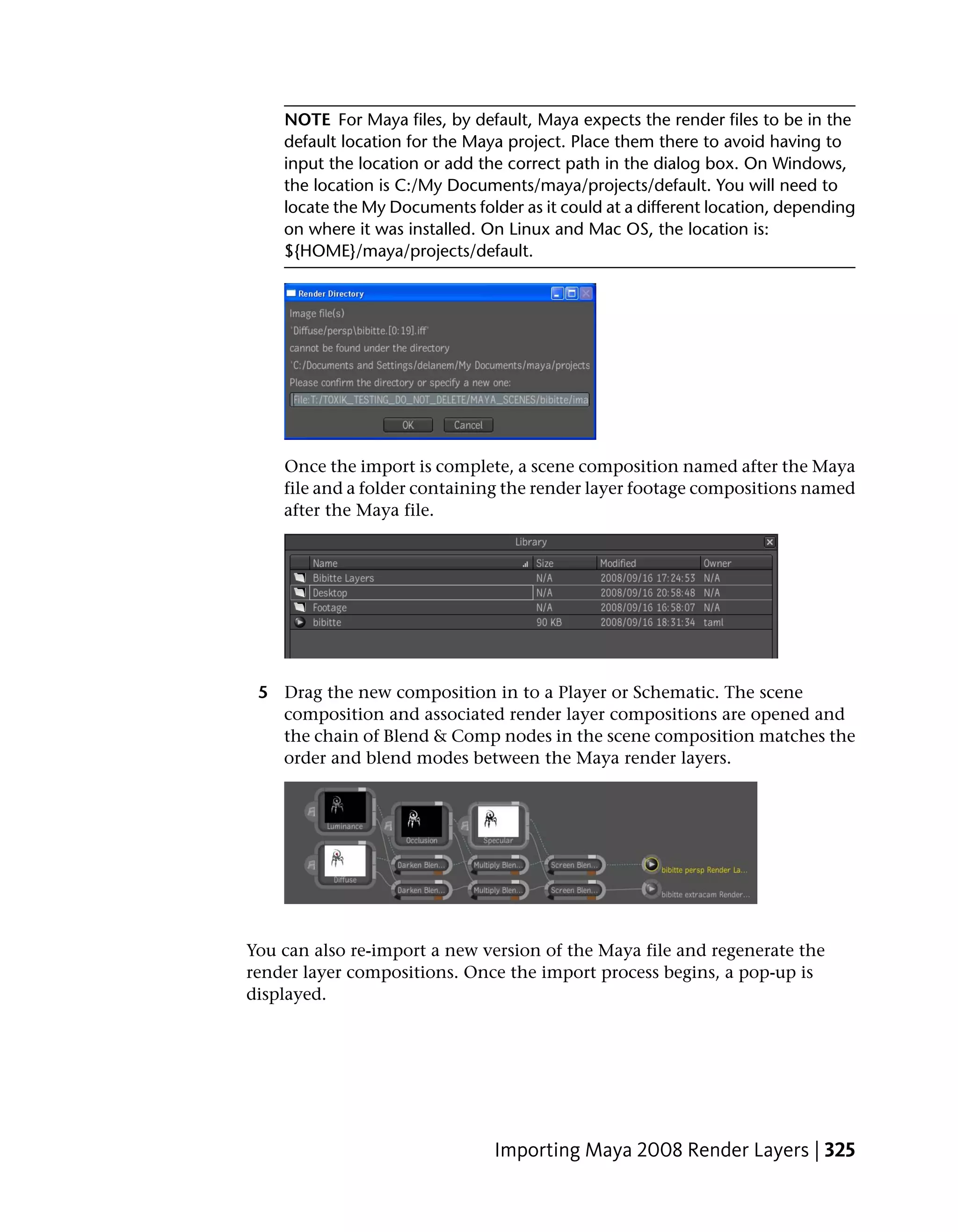
346 | Chapter 15 2D Compositing](https://image.slidesharecdn.com/mayacompositeuserguide-1260452105-phpapp01/75/Mayacompositeuserguide-362-2048.jpg)
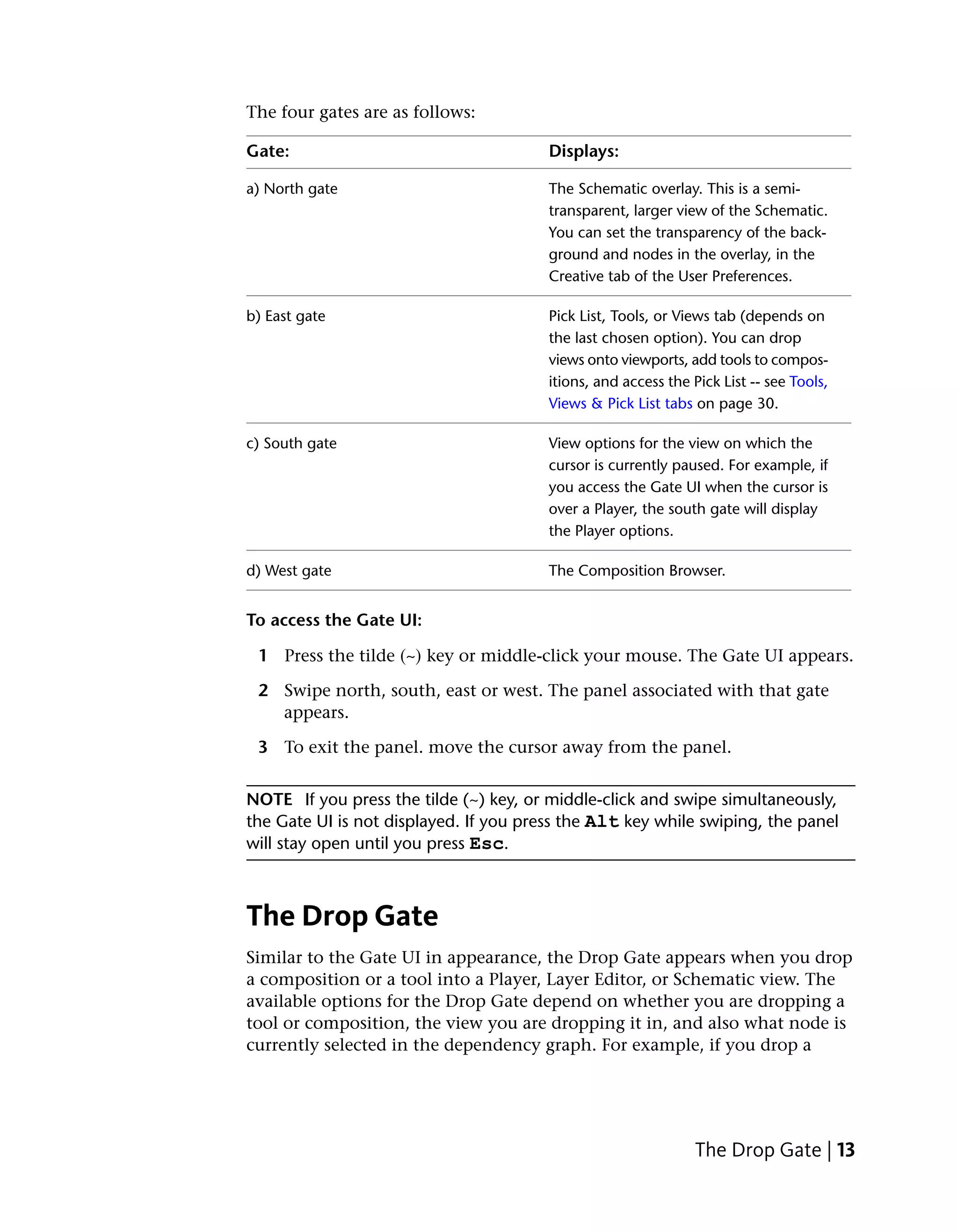
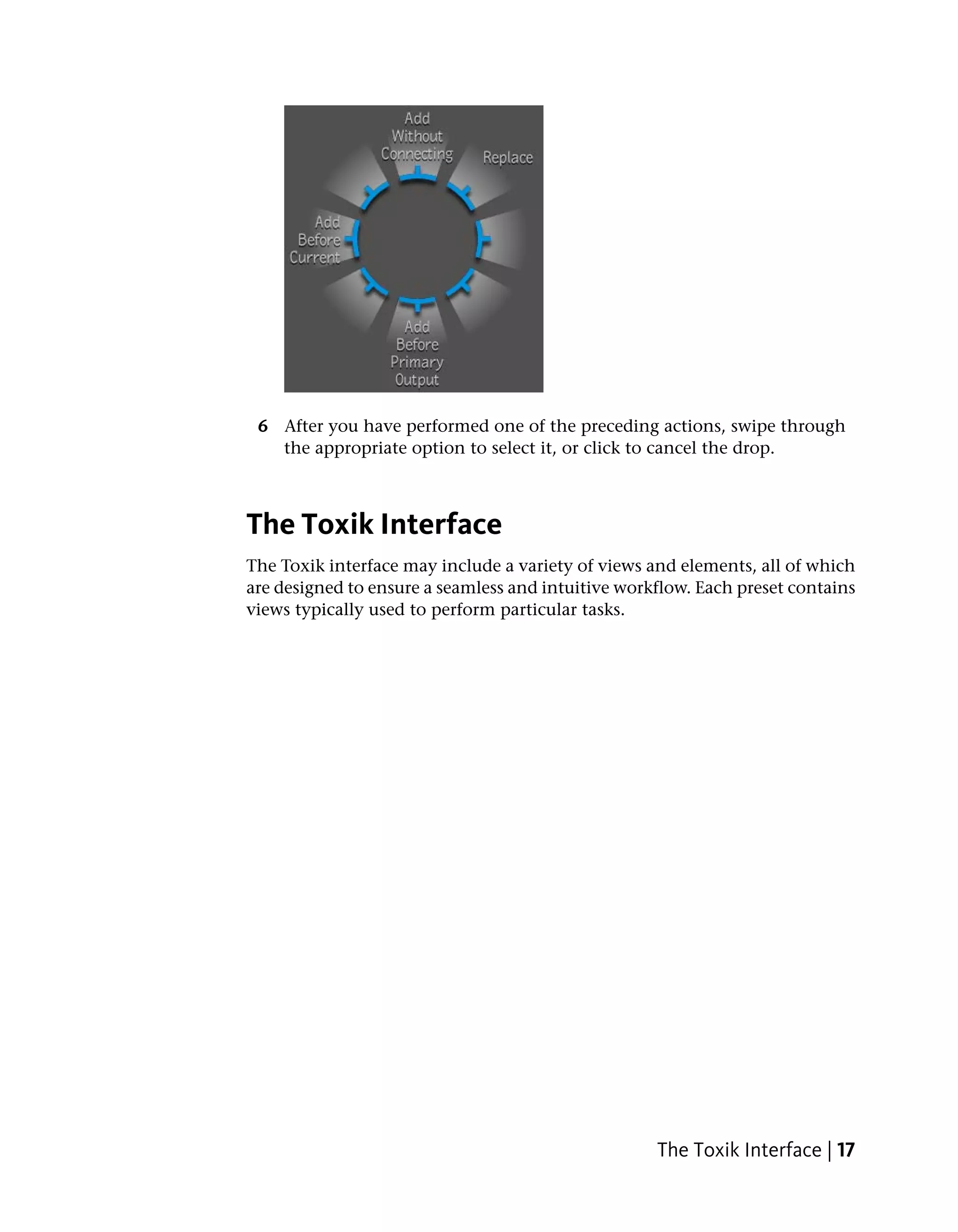
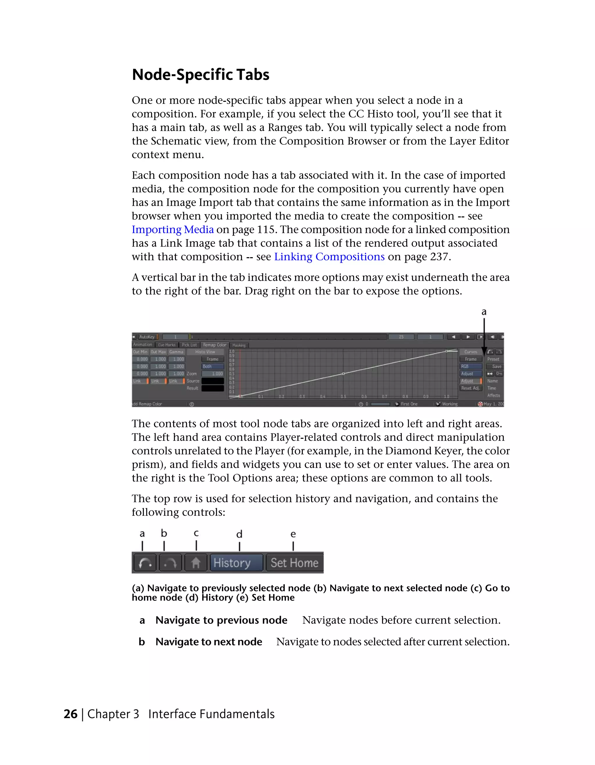
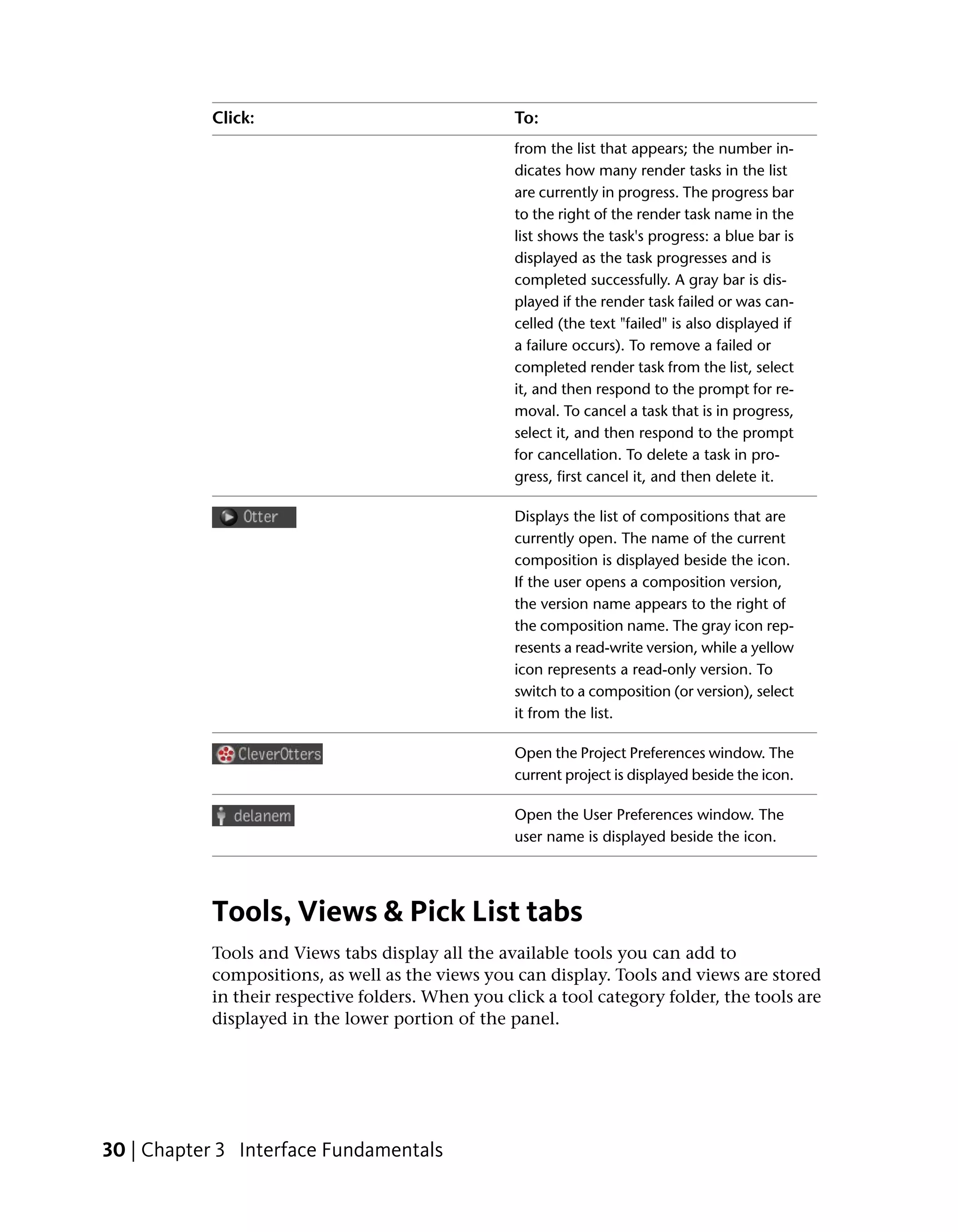
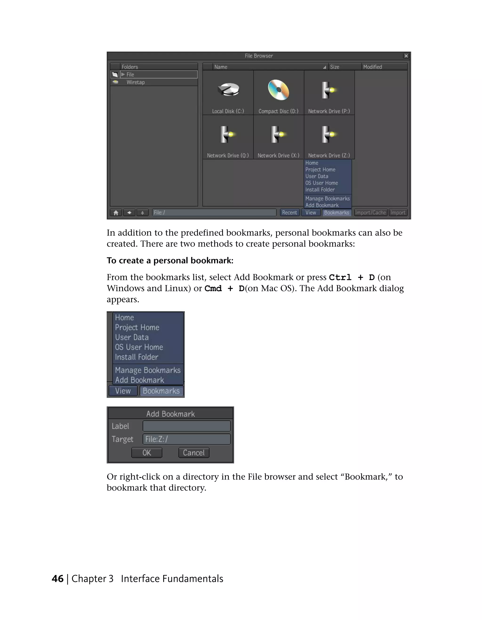
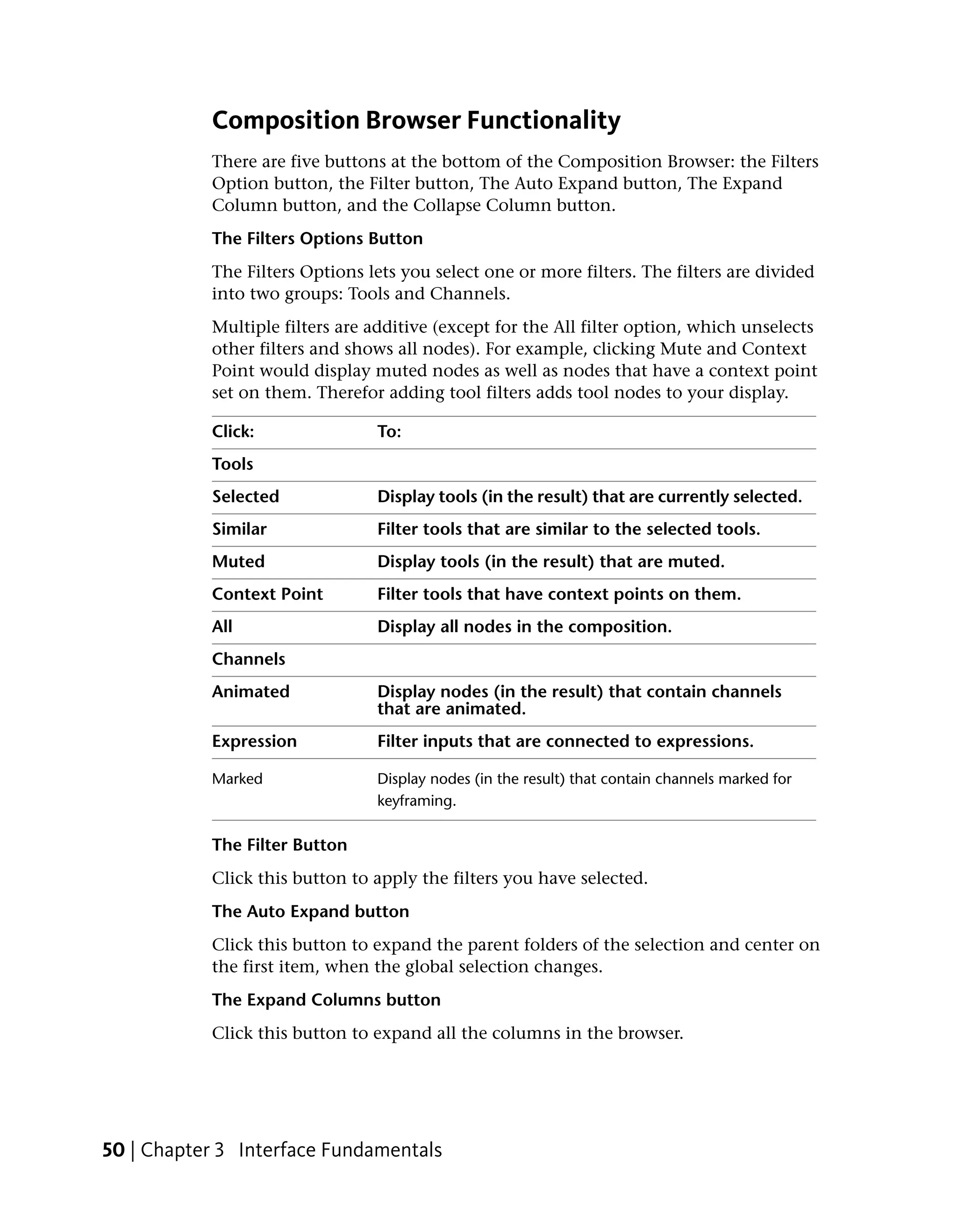
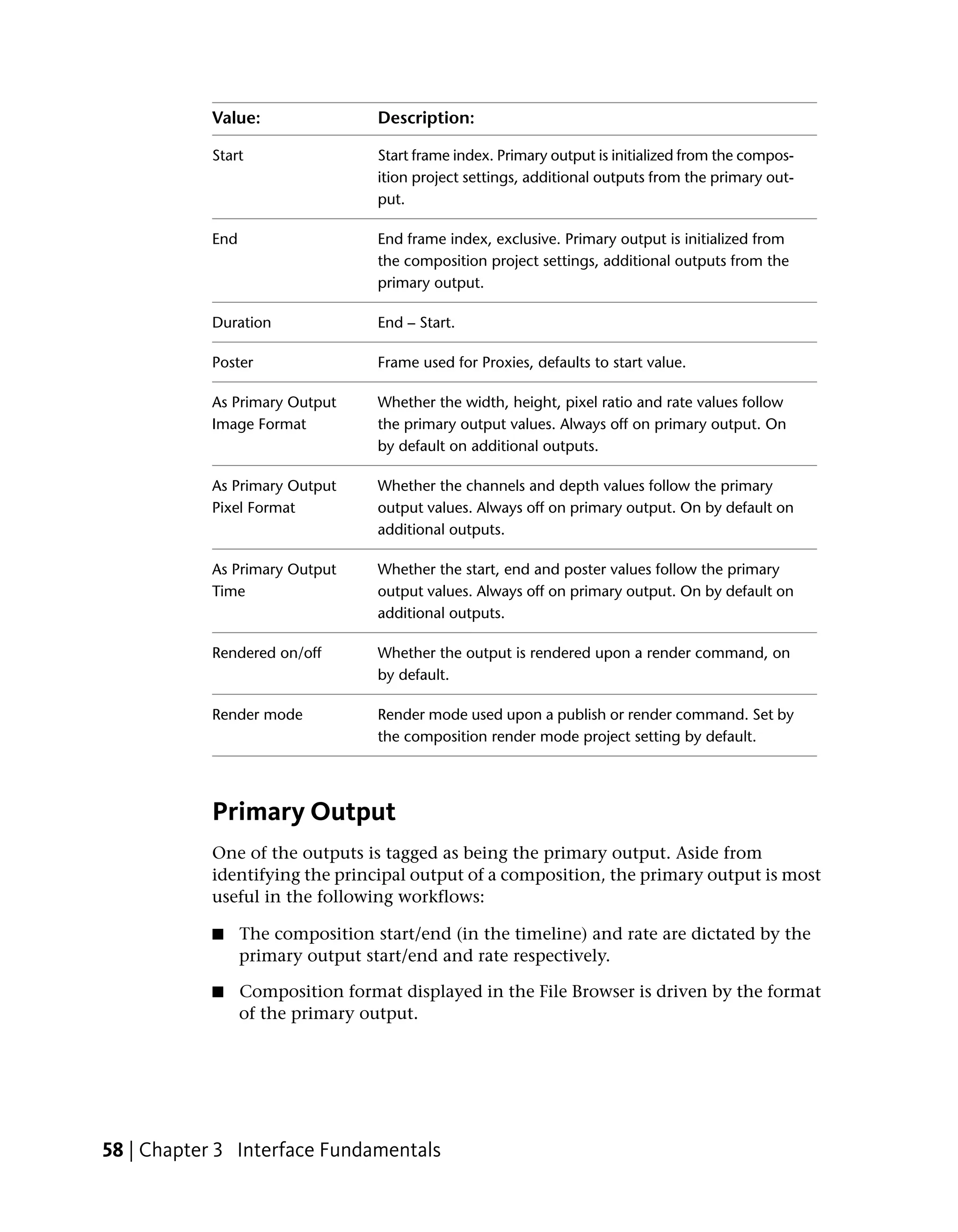
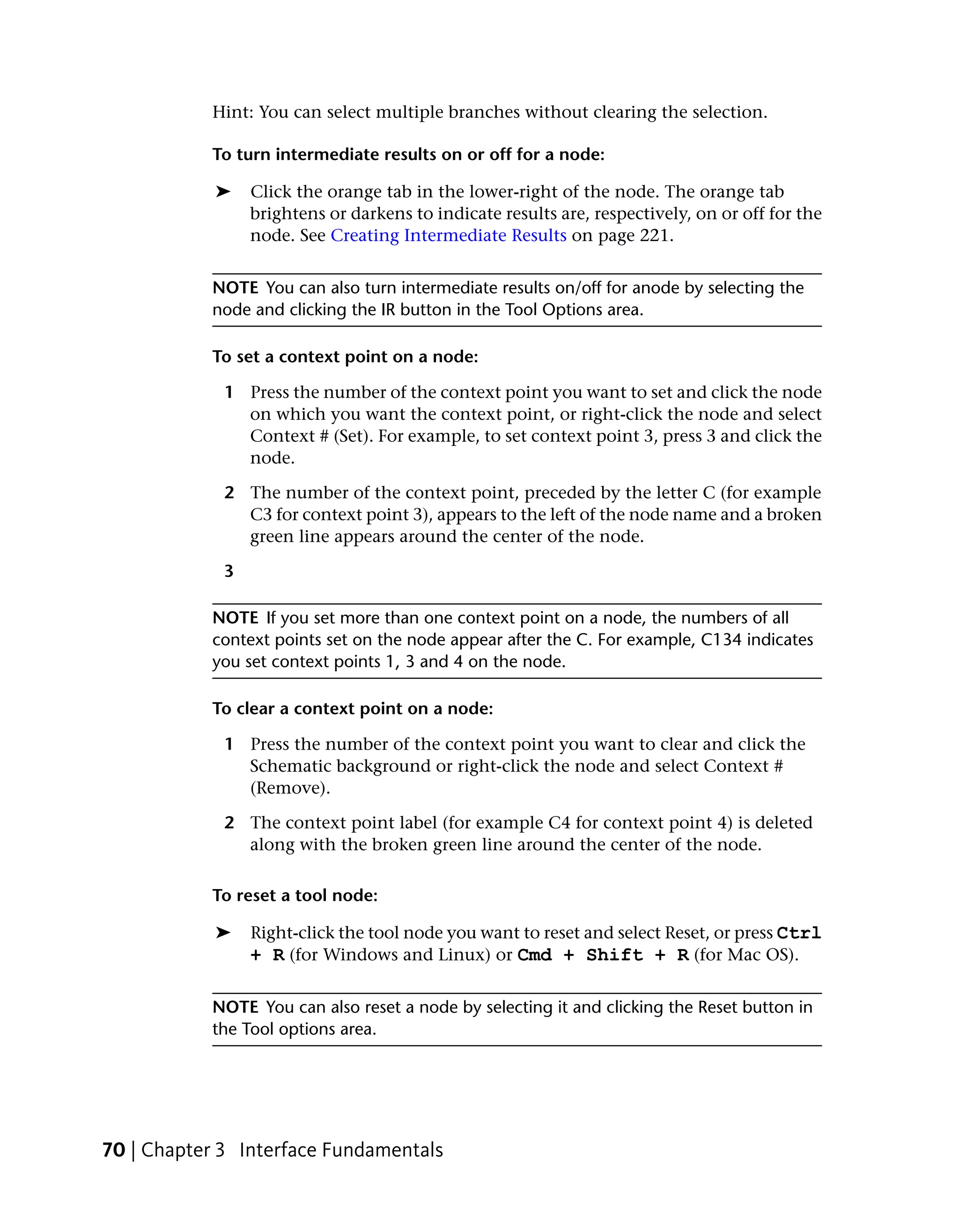
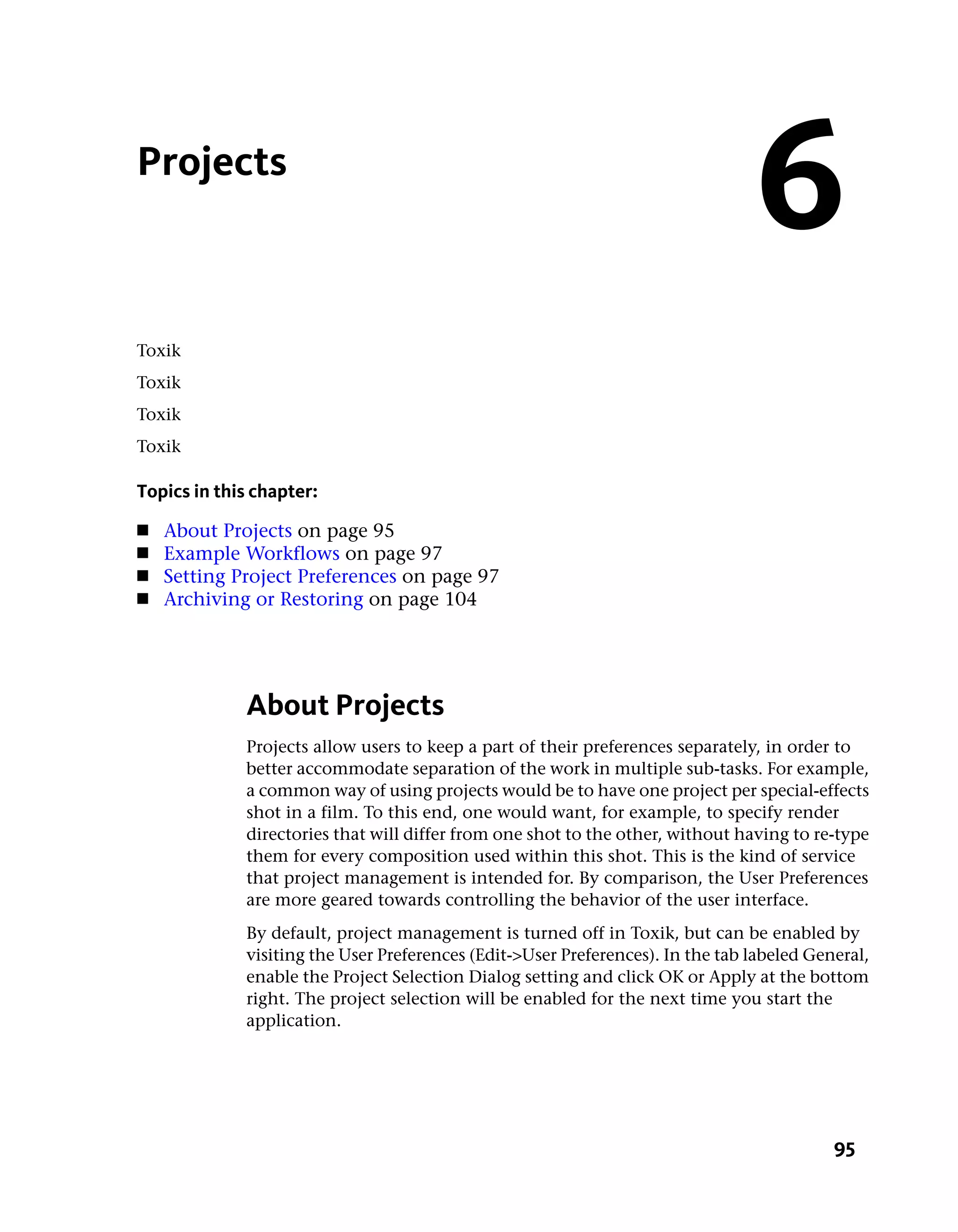
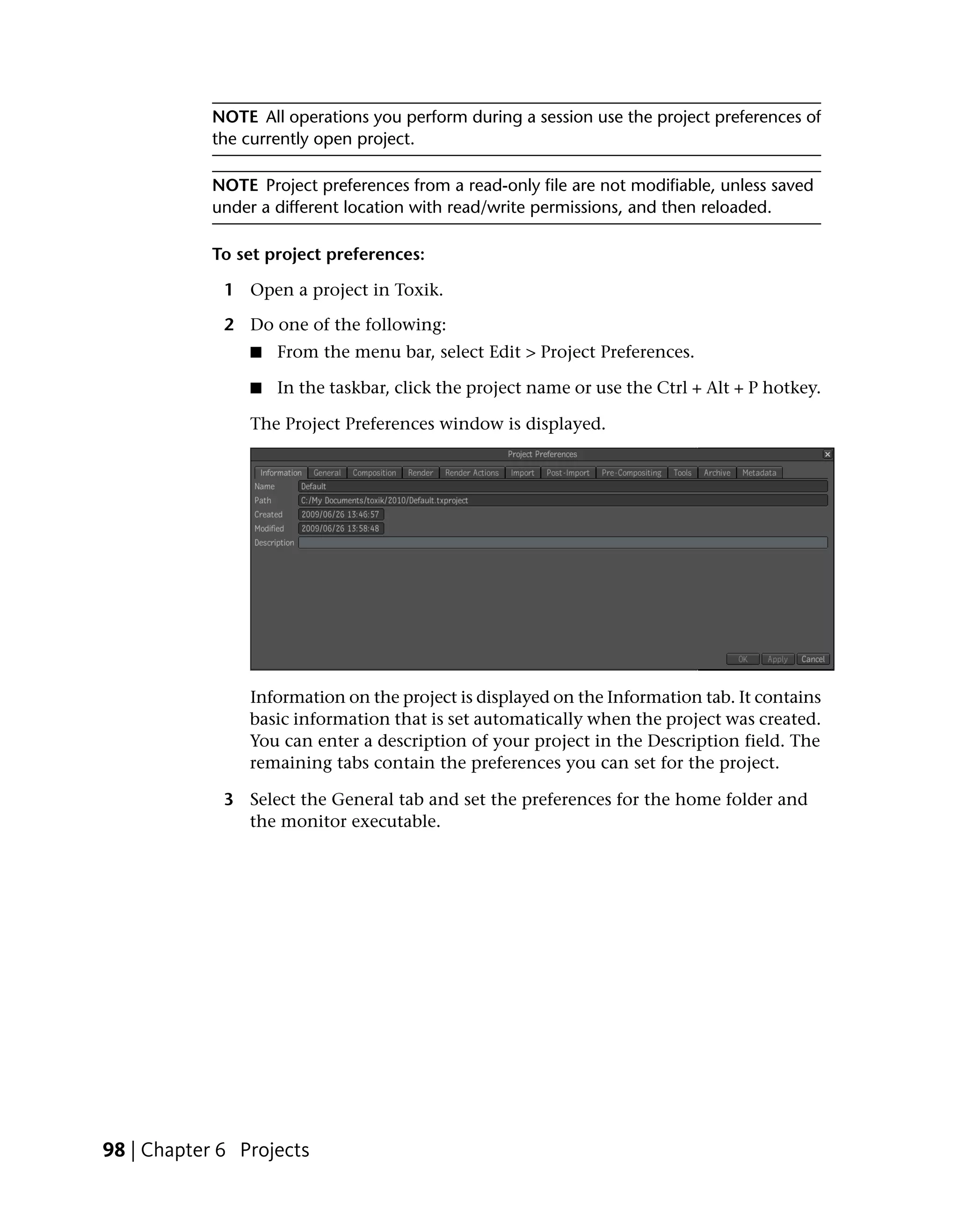
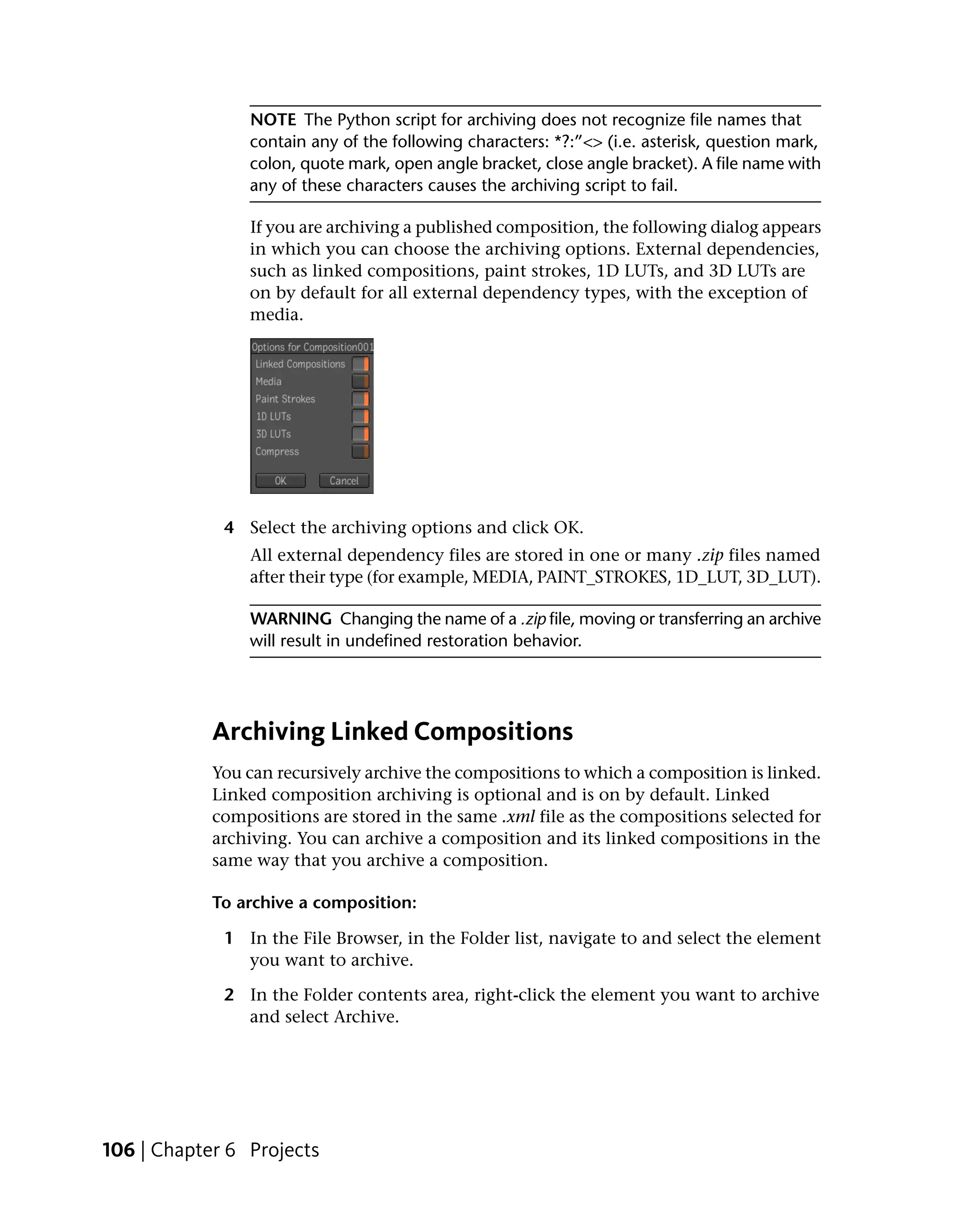
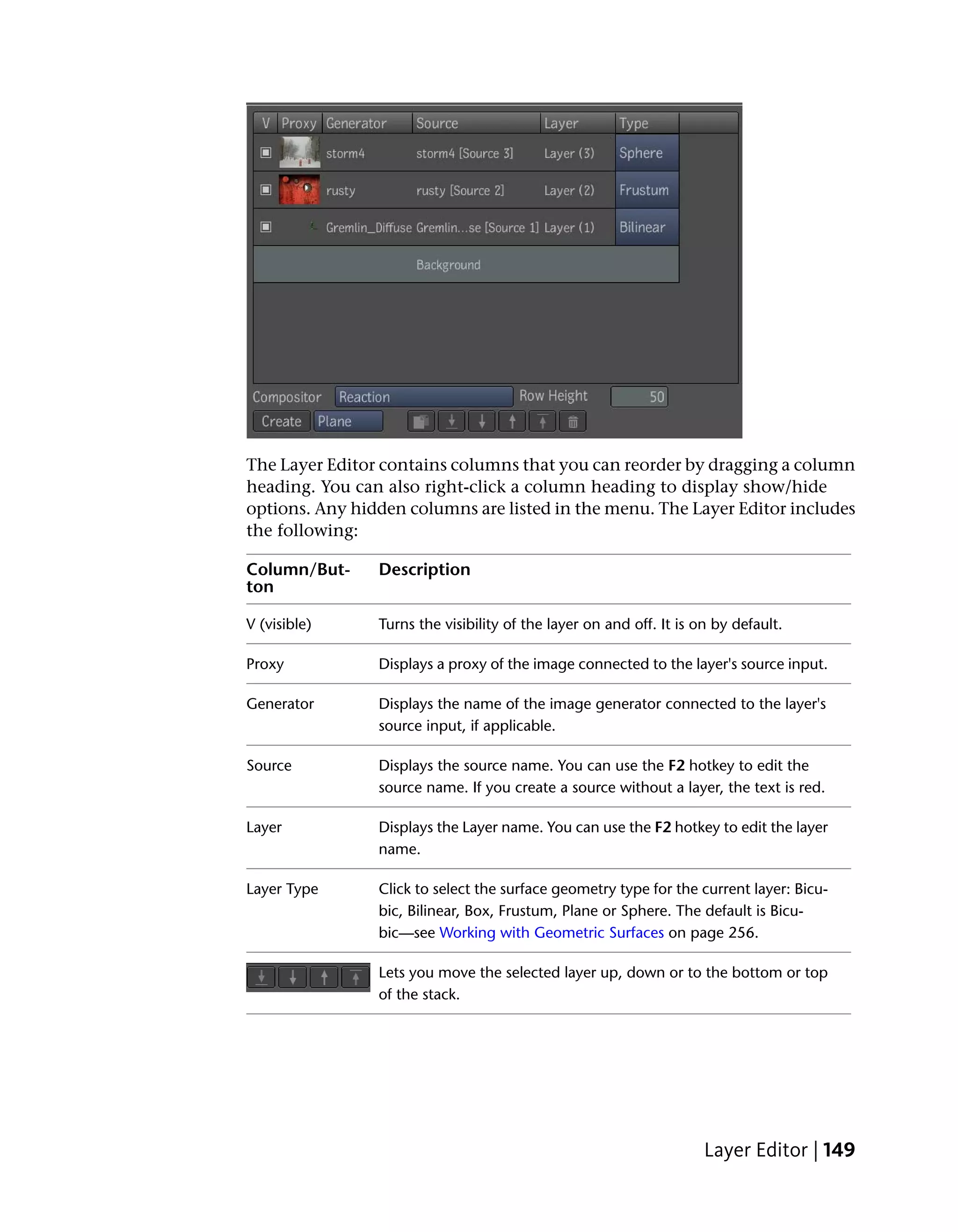
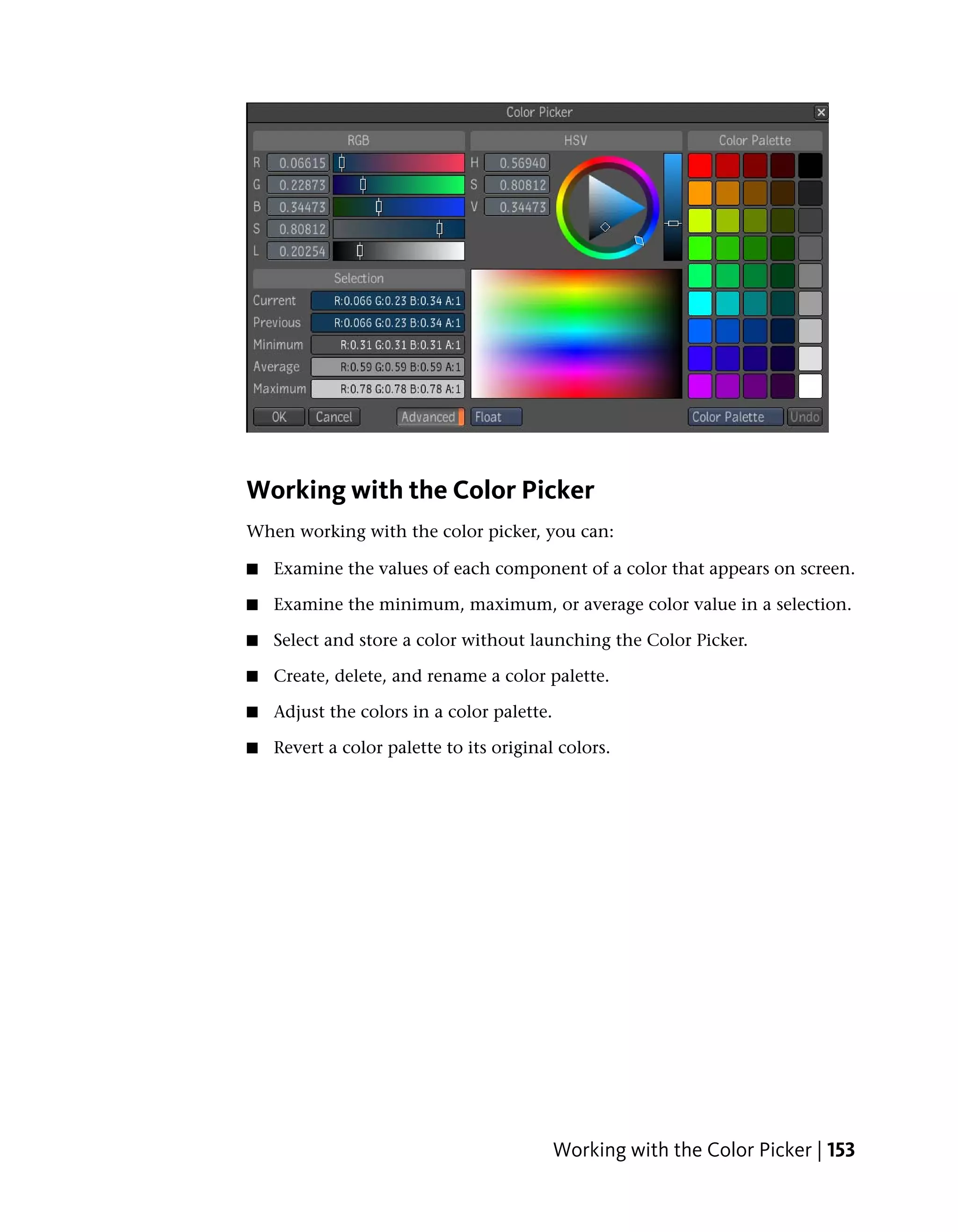
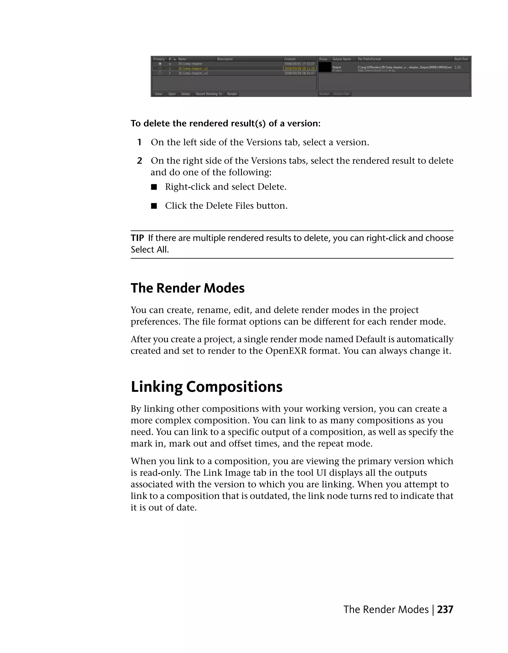
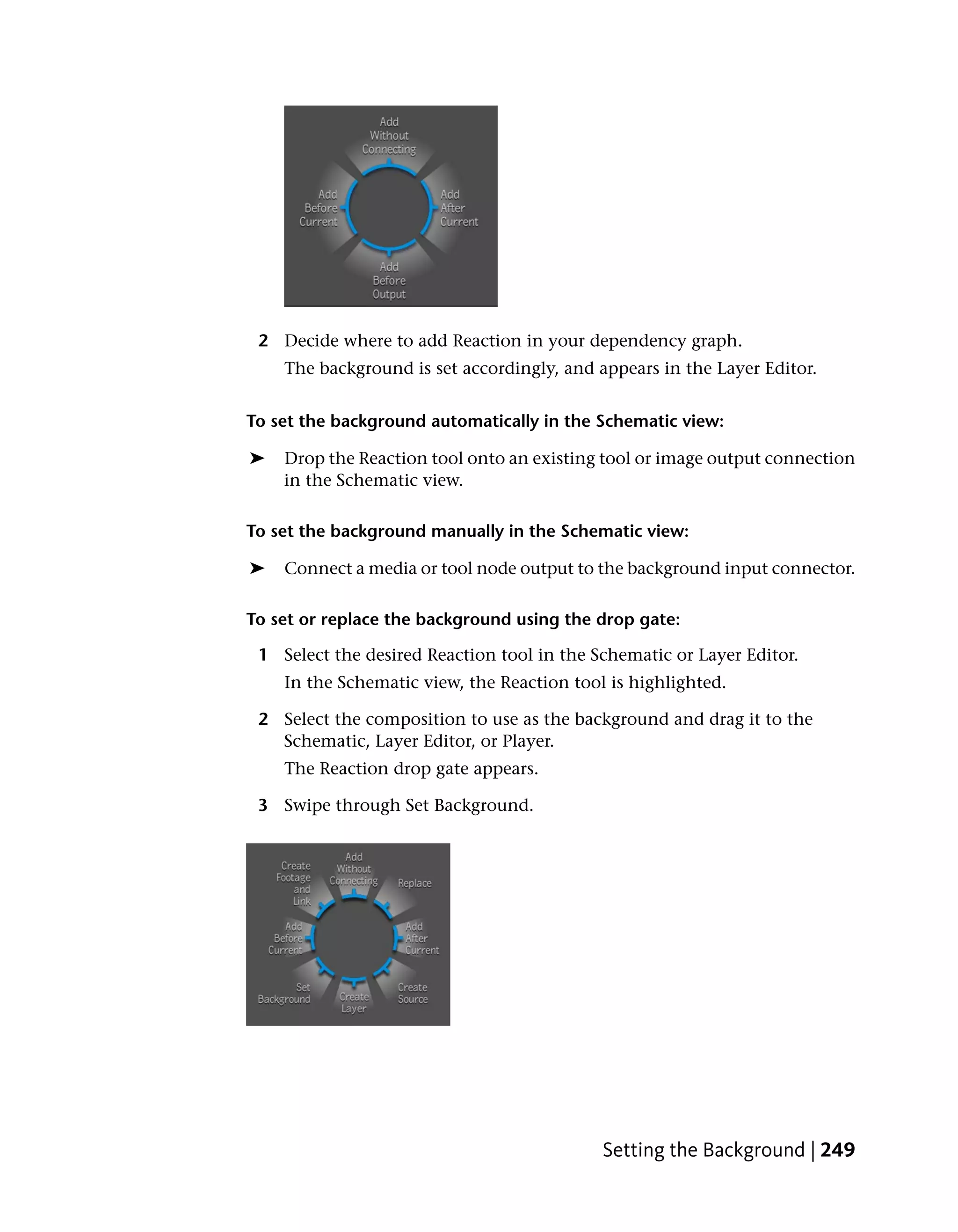
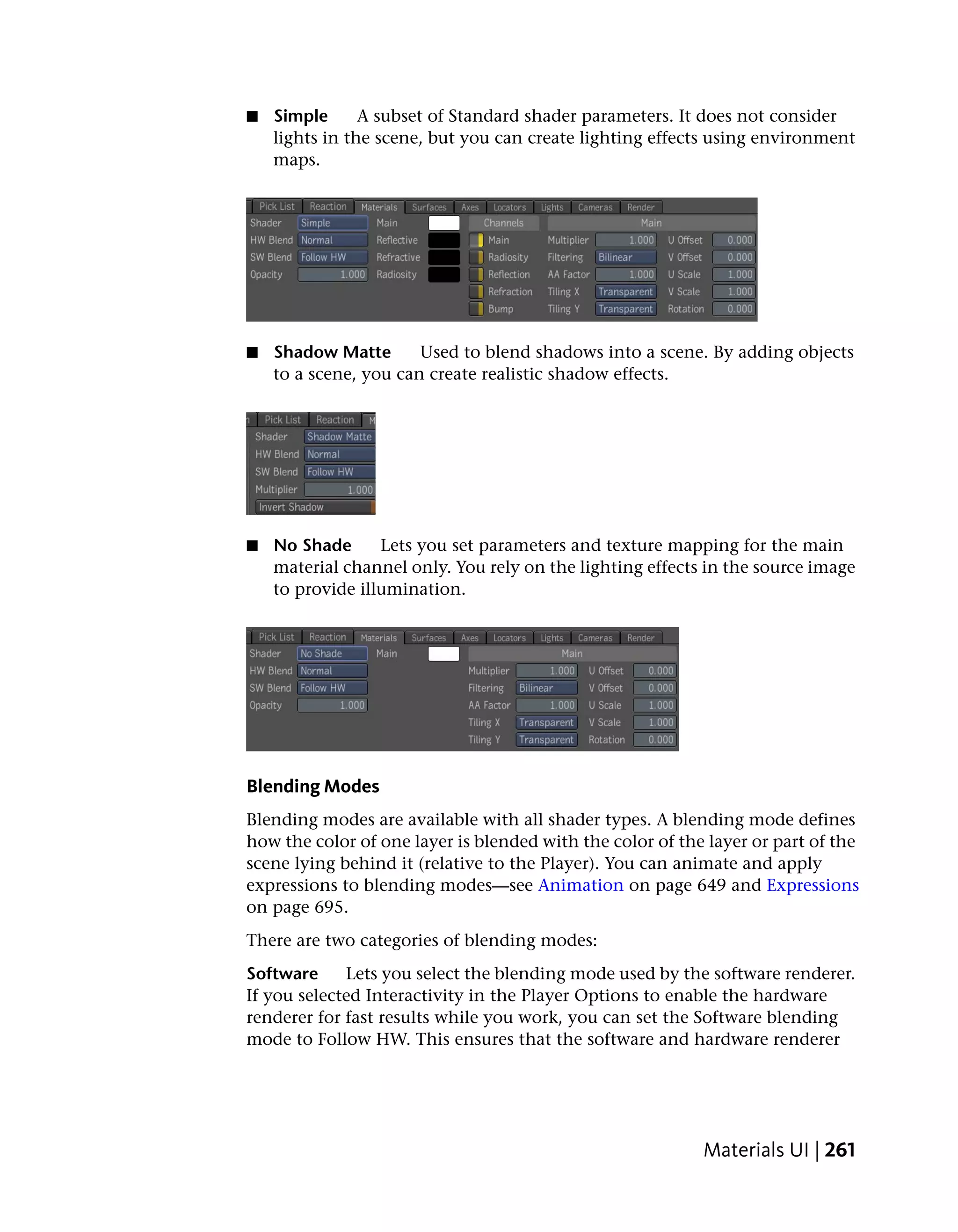
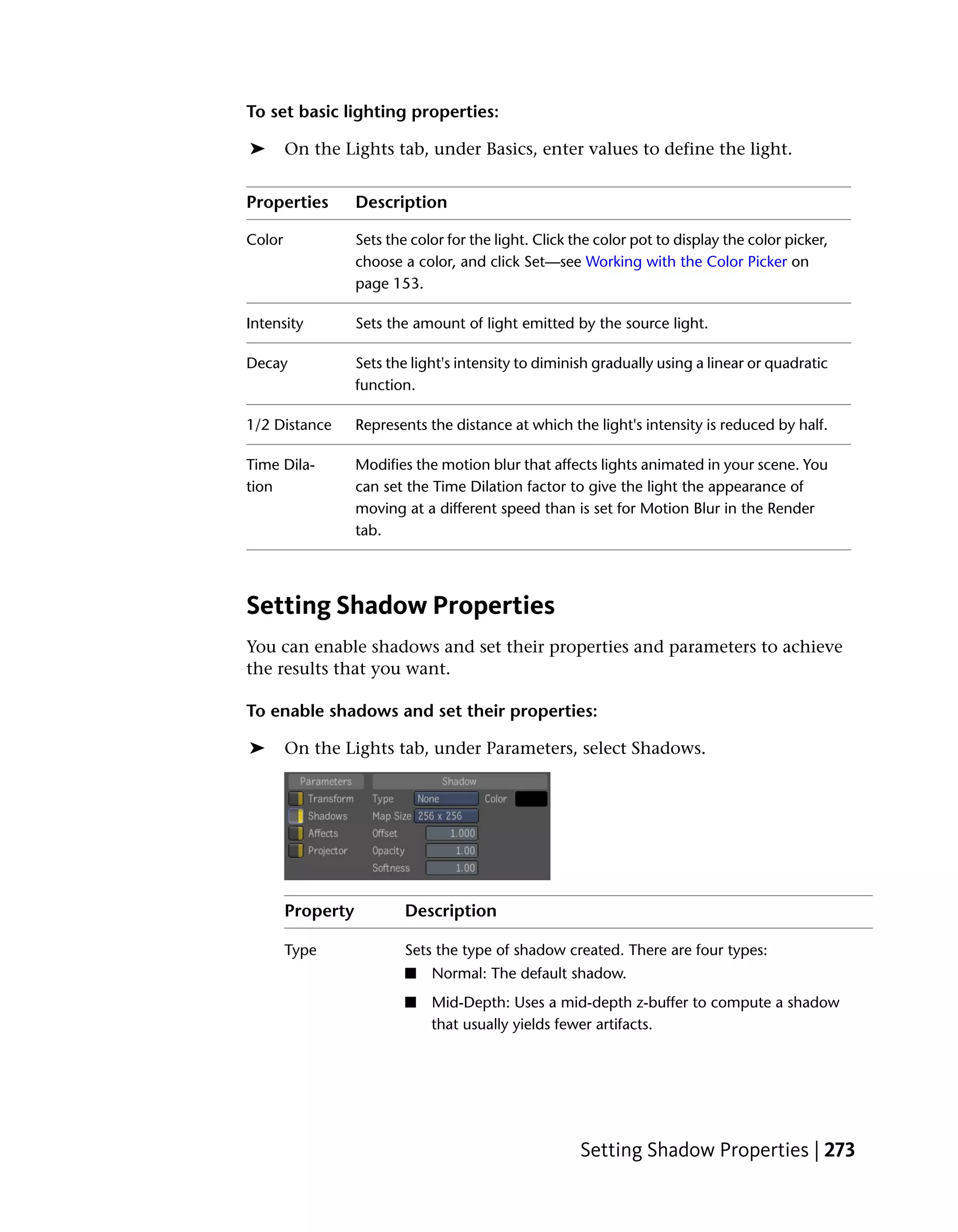
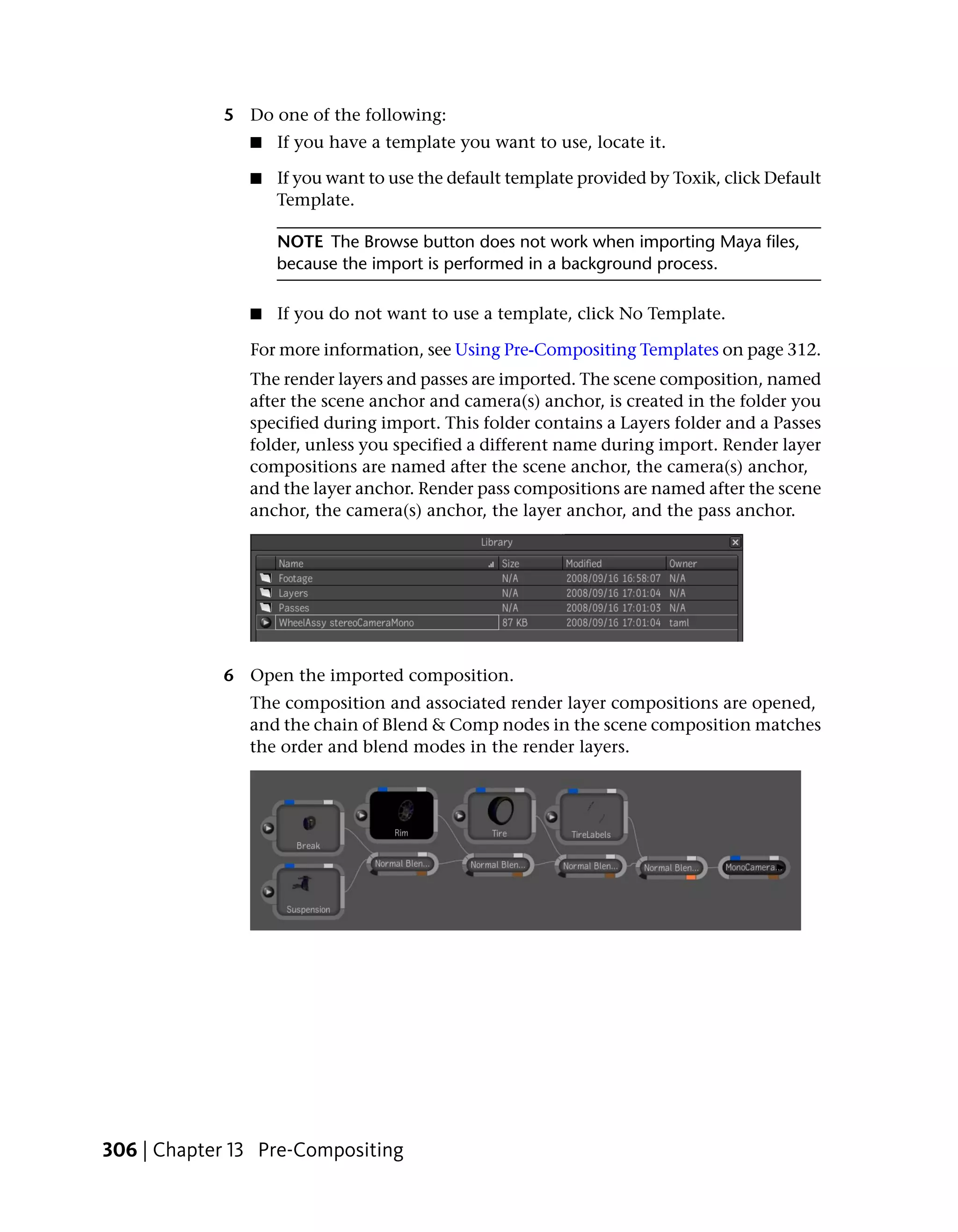
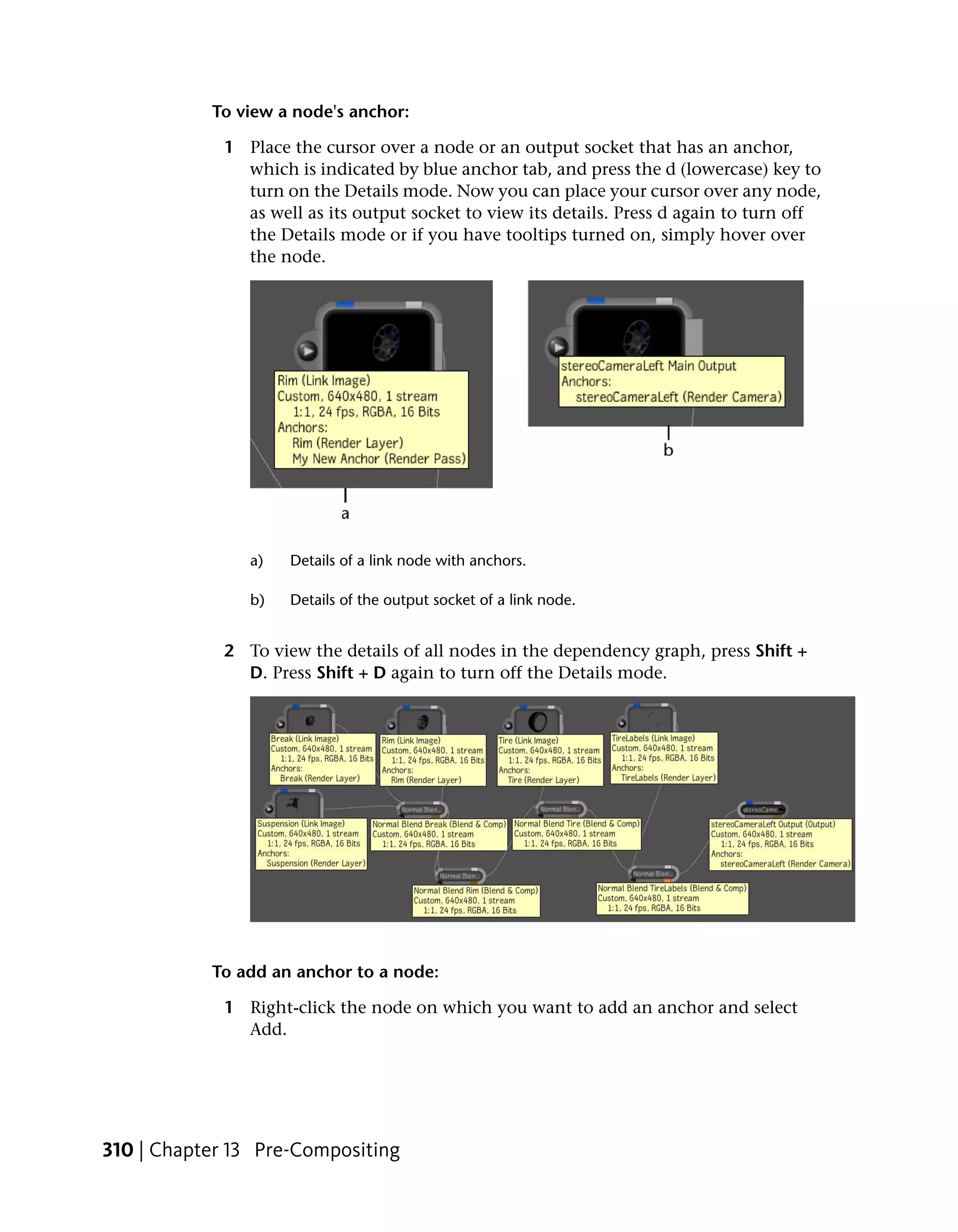
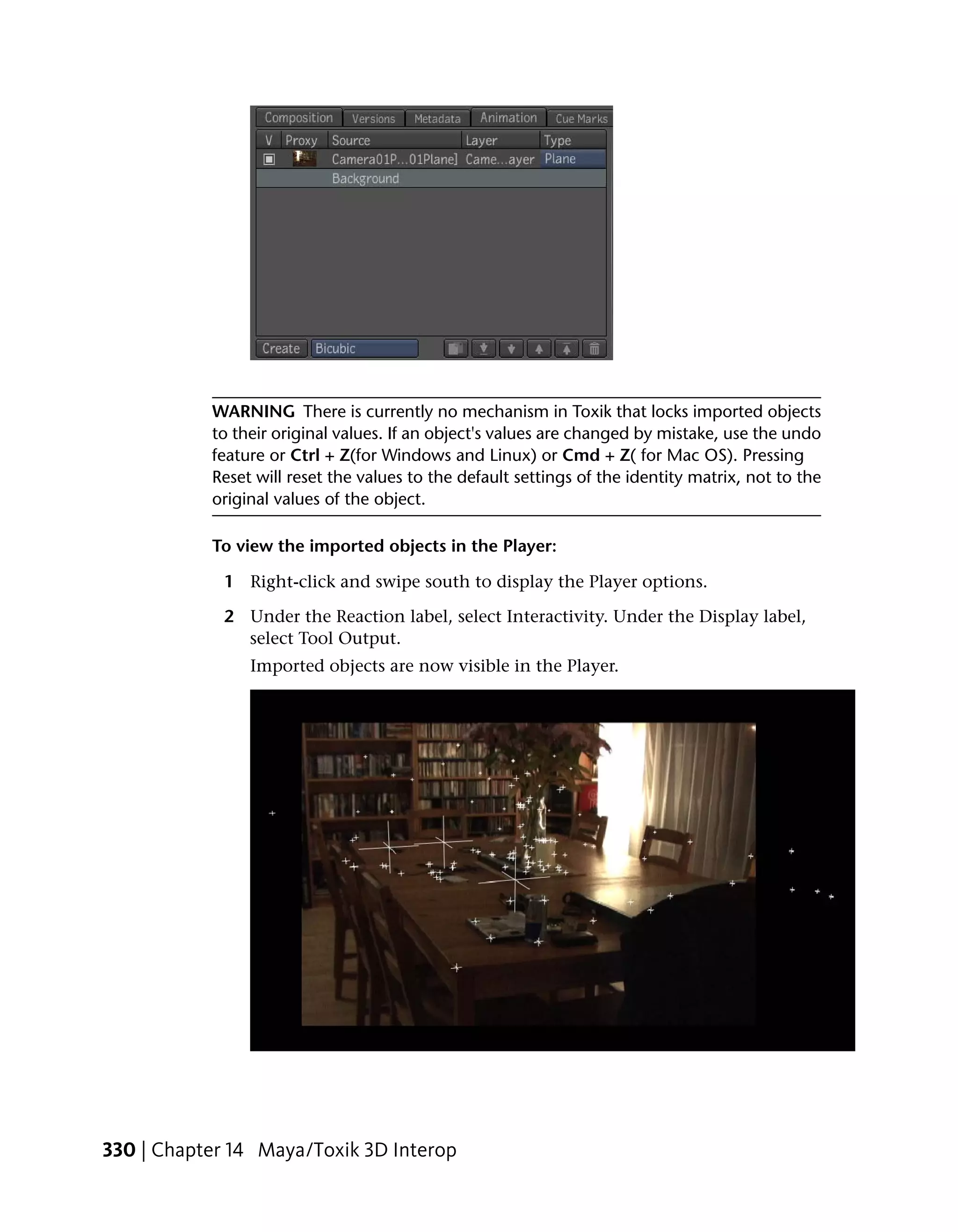
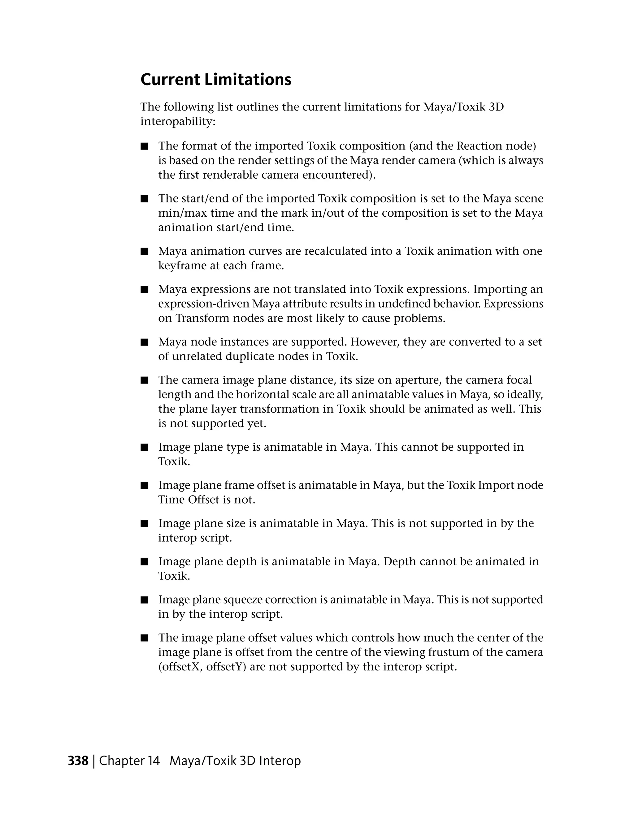
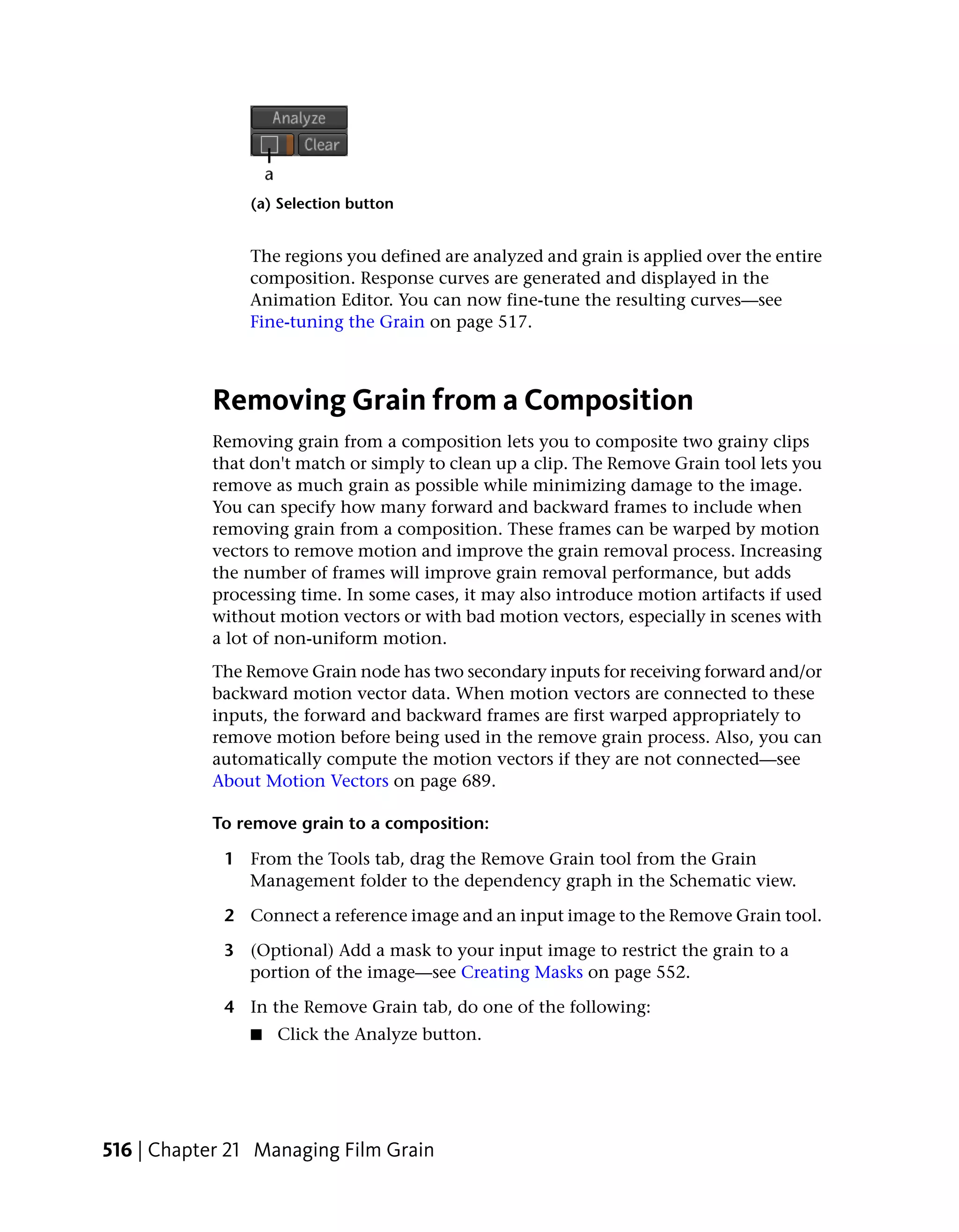
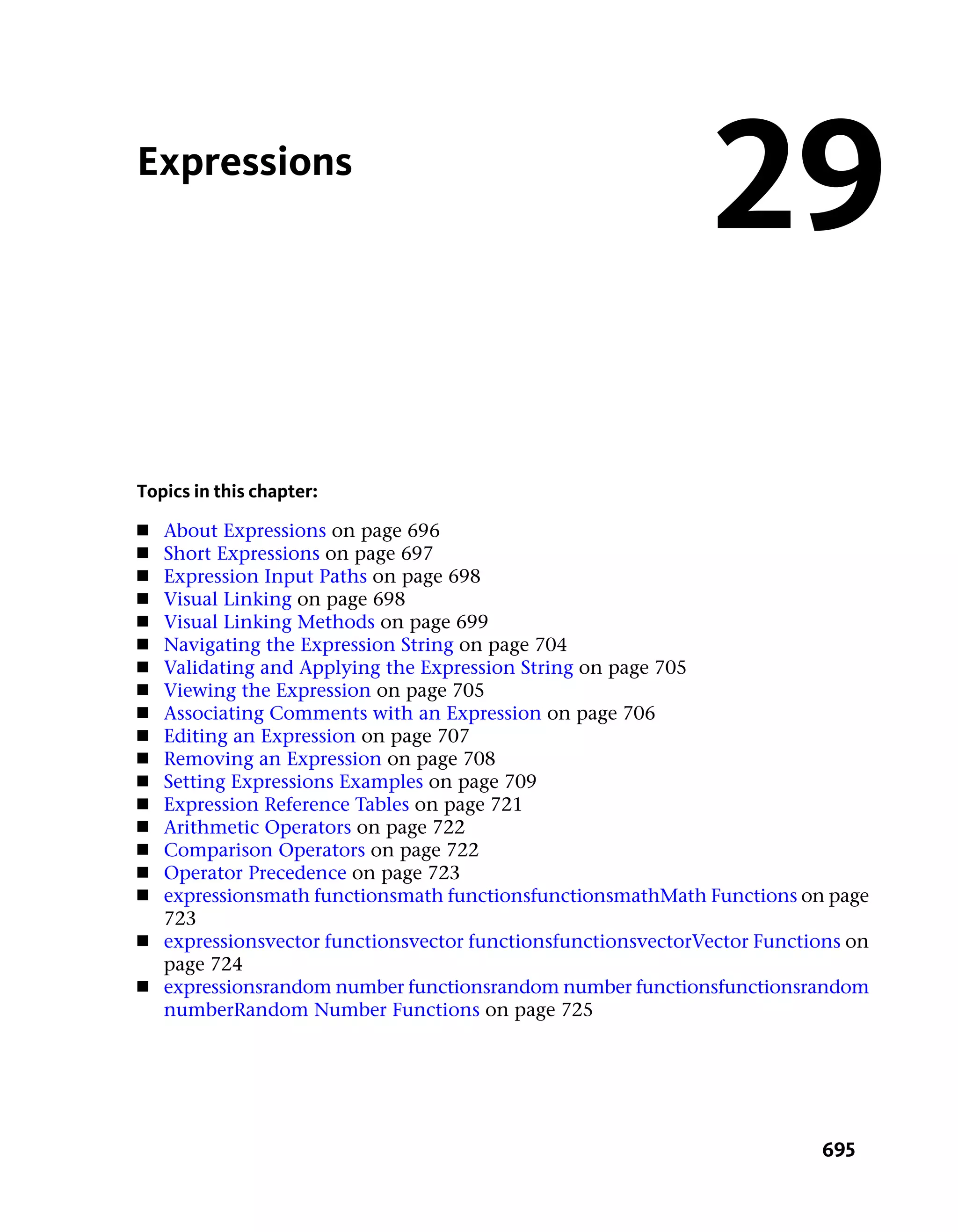
![■ Front Channel Selects which channel to use for the front. Channel
selections include Luma, Red, Green, Blue, and Alpha (default is Alpha).
■ Front Invert Inverts the front before using it (default is off).
■ Front Intensity Specifies the intensity of the front layer (default is 100%;
range is [0,10]).
■ Front Opacity Controls the opacity of the front in the blending. If a
matte image is also used to control the blending, the two are multiplied
together. This parameter is never ignored (default is 100%; range is [0,1]).
■ Back Channel Selects which channel to use for the back. Channel
selections include Luma, Red, Green, Blue, and Alpha (default is Alpha).
■ Back Invert Inverts the back before using it (default is off).
■ Back Intensity Specifies the intensity of the back layer (default is 100%;
range is [0,10]).
■ Matte Channel Selects which channel to use for the matte. Channel
selections include Luma, Red, Green, Blue, and Alpha (default is Alpha).
■ Matte Invert Inverts the matte before using it (default is off).
■ Matte Ignore Determines whether or not the matte input is used to
modulate the blend. The default is false (meaning that the matte input
will be used in the blending equations). Note that if the Matte Input is not
chain connected, it will be automatically ignored (no feedback needs to
be provided in the UI).
■ Blend Mode Determines which blend mode will be used (the default is
Normal).
Click the Blend button to view other available modes.
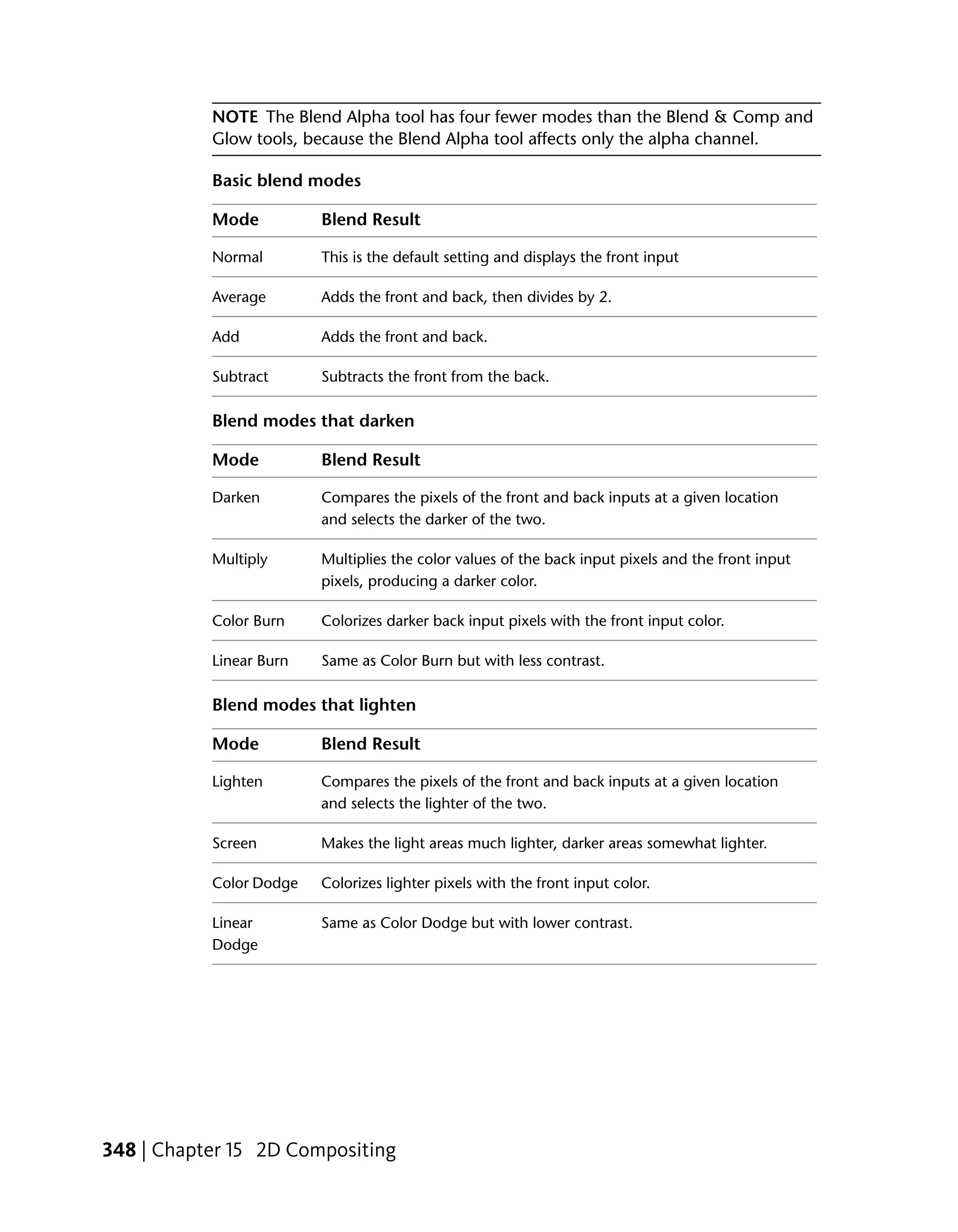
Blend Modes
The following tables (grouped by type) list the available blend modes and
describe the resulting blend effect.
Blend Alpha | 347](https://image.slidesharecdn.com/mayacompositeuserguide-1260452105-phpapp01/75/Mayacompositeuserguide-363-2048.jpg)
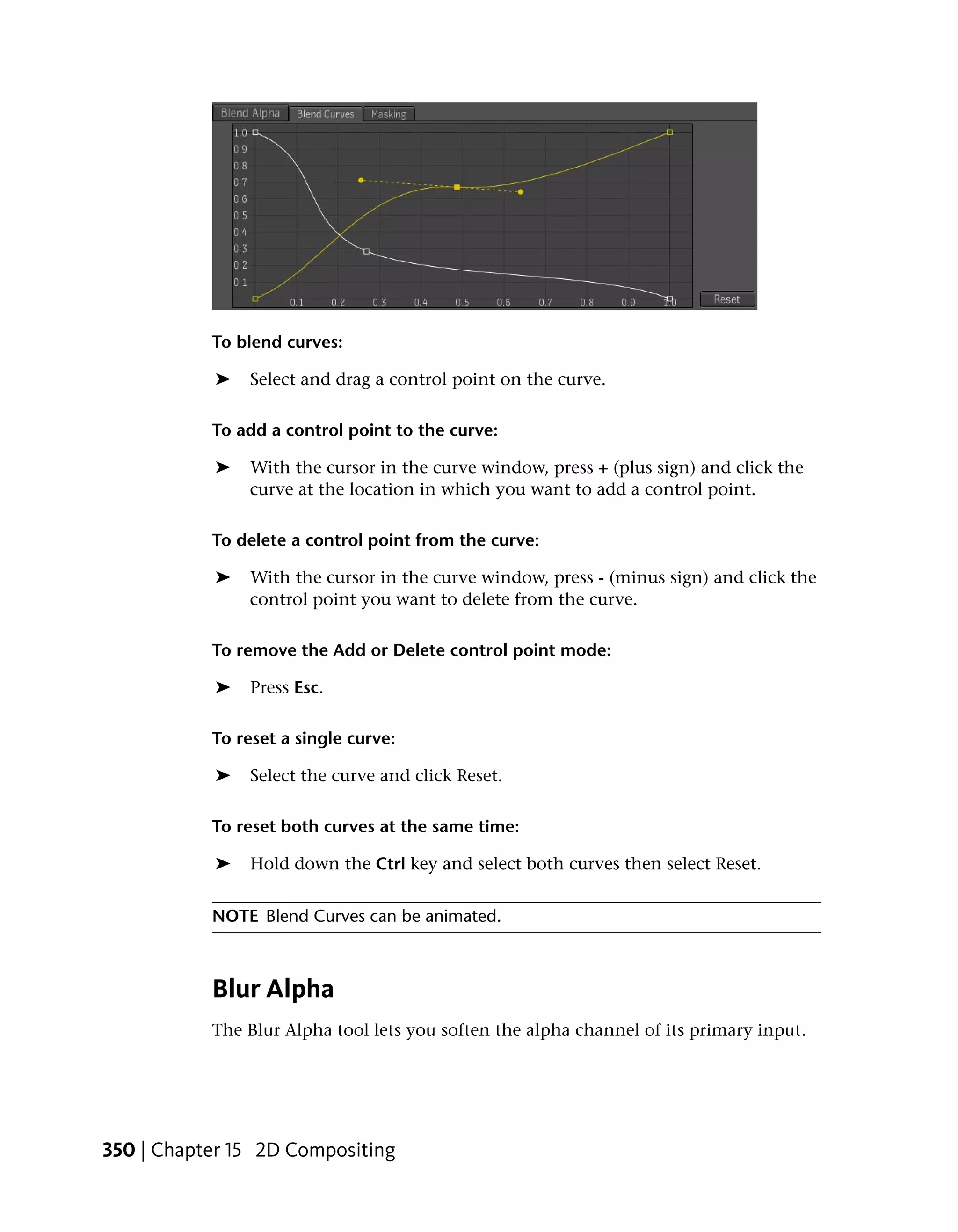
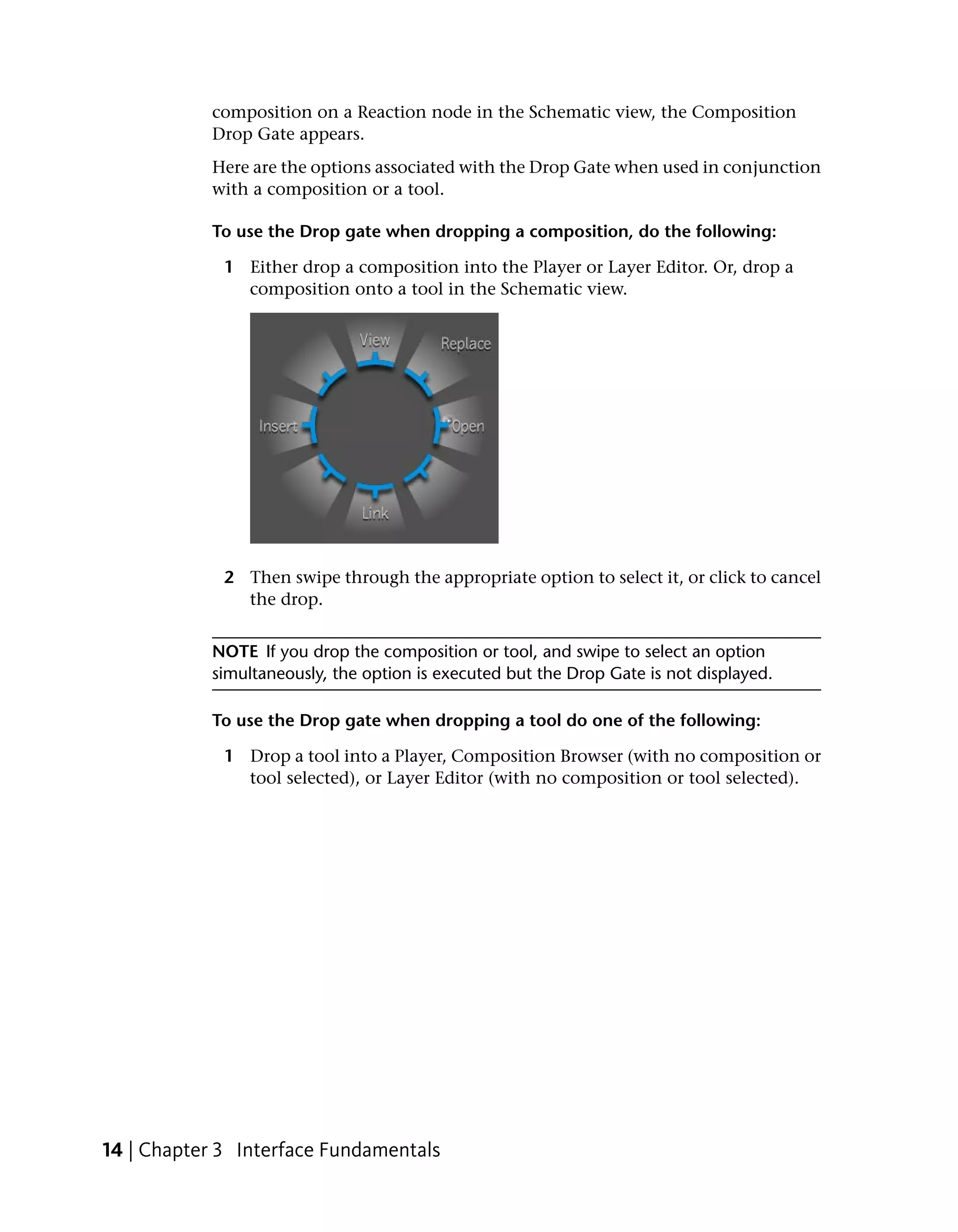
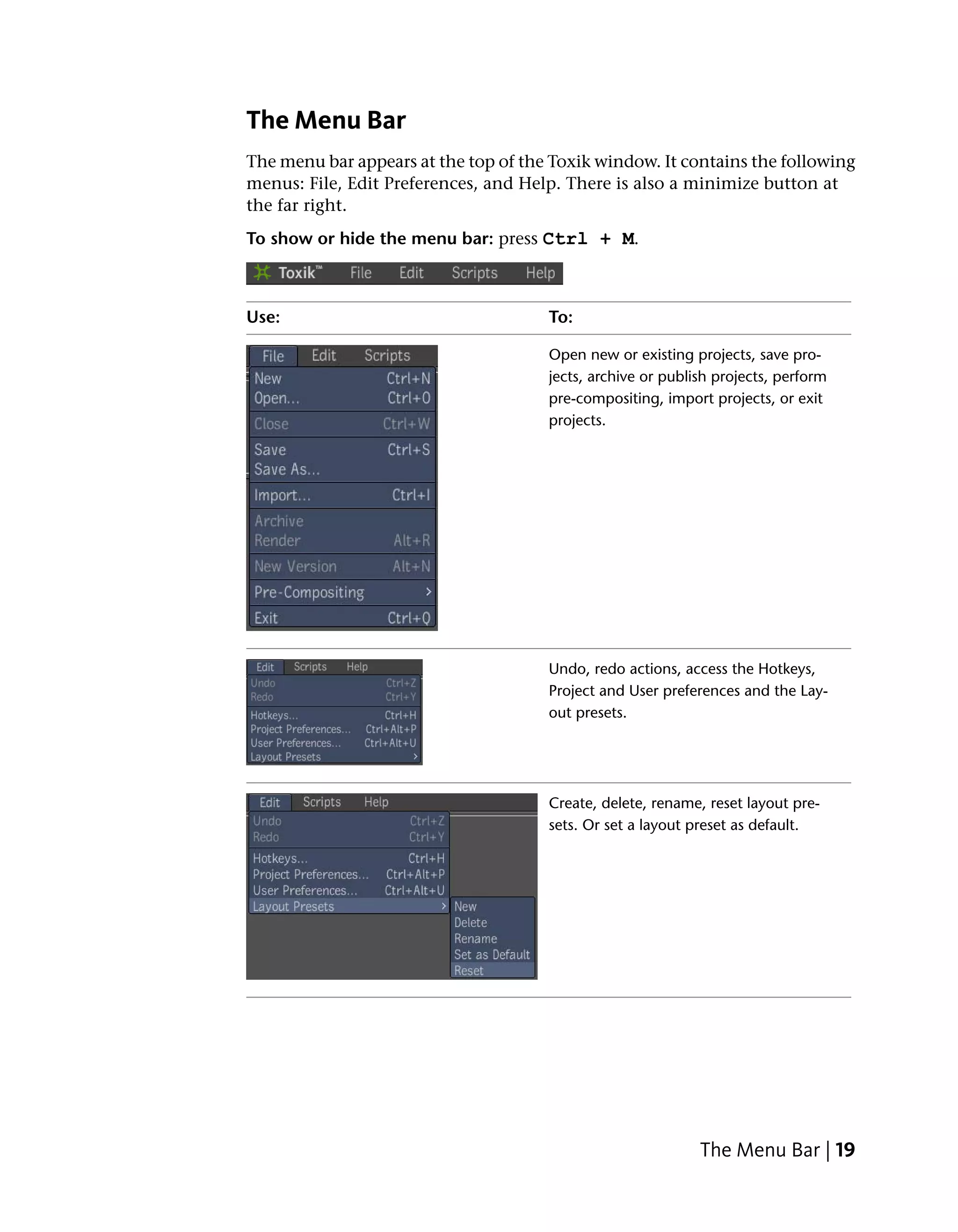
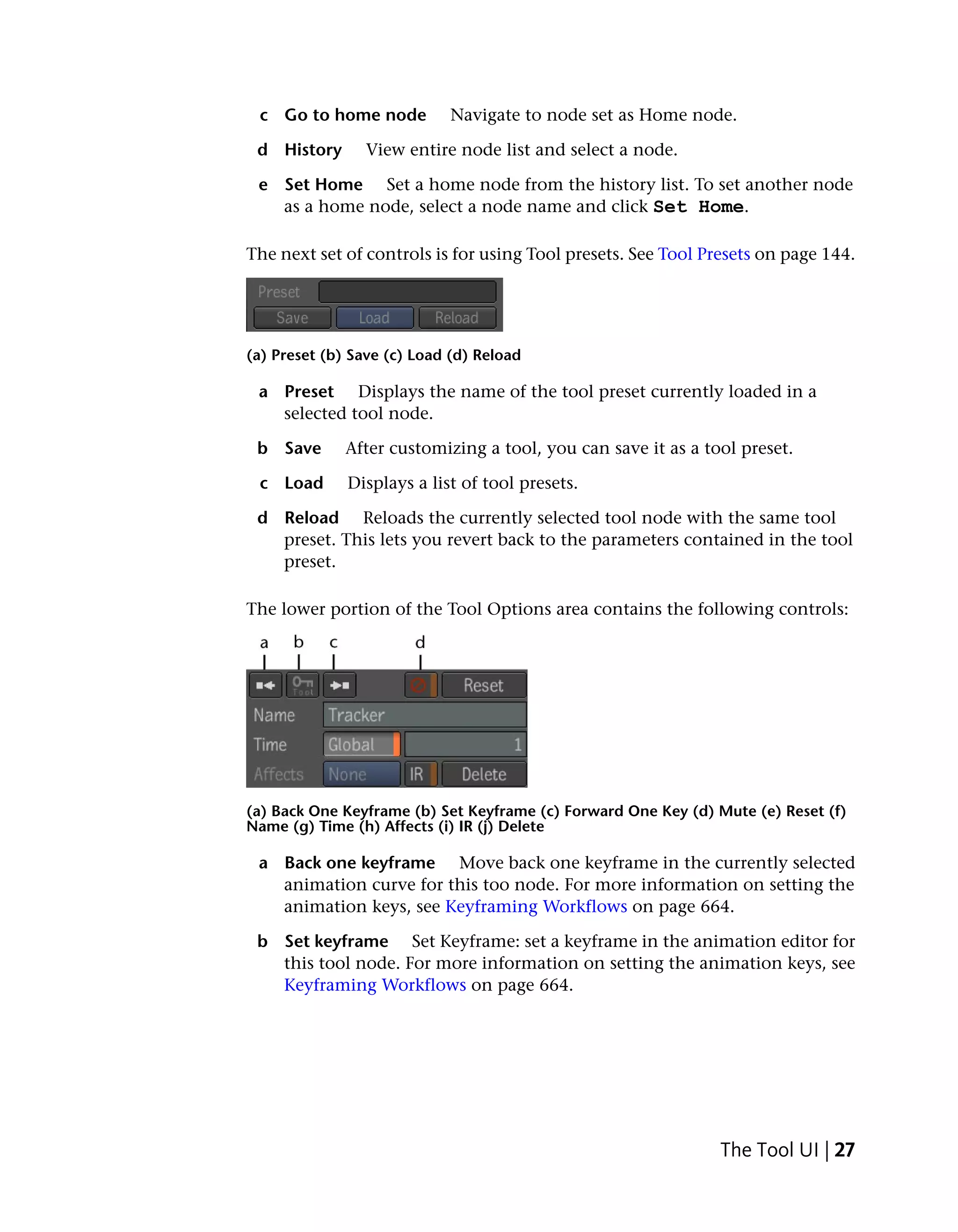
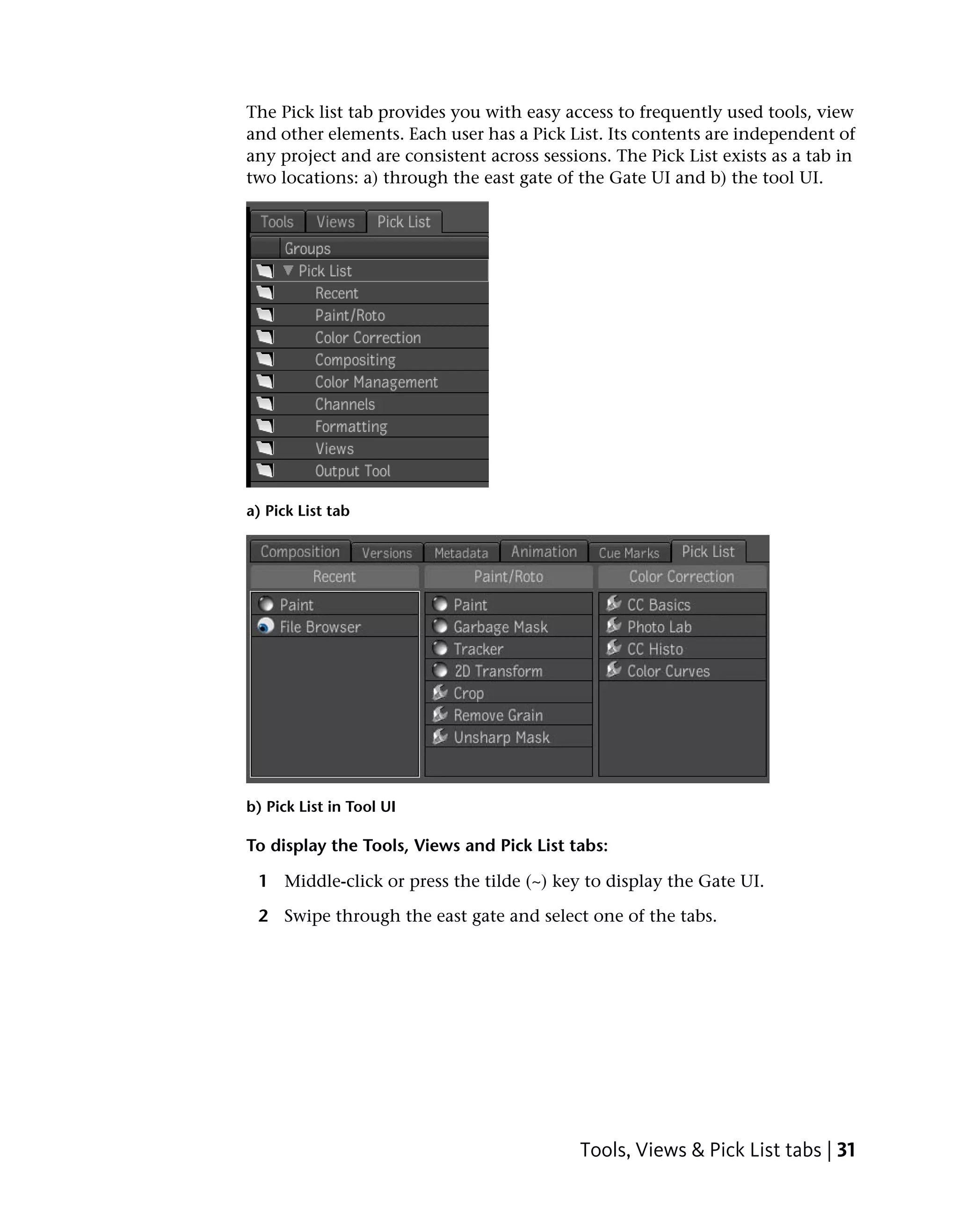
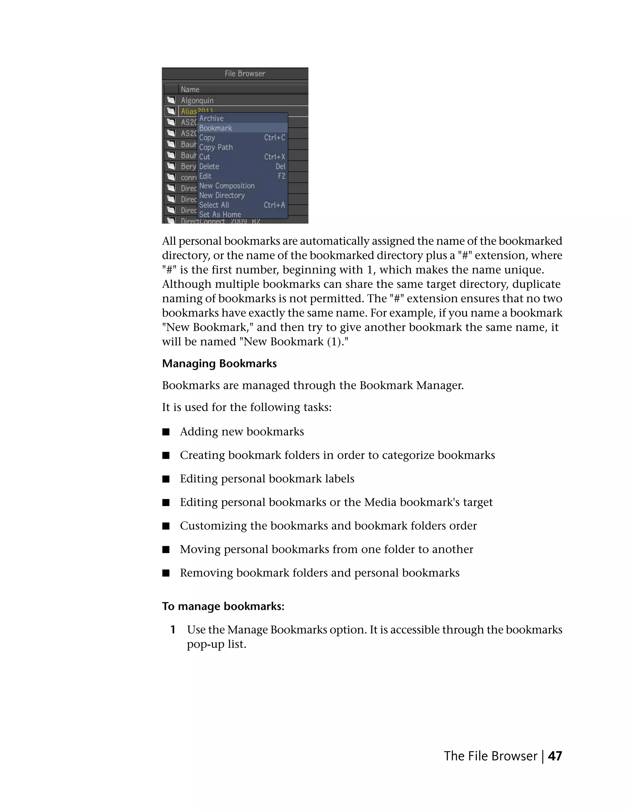
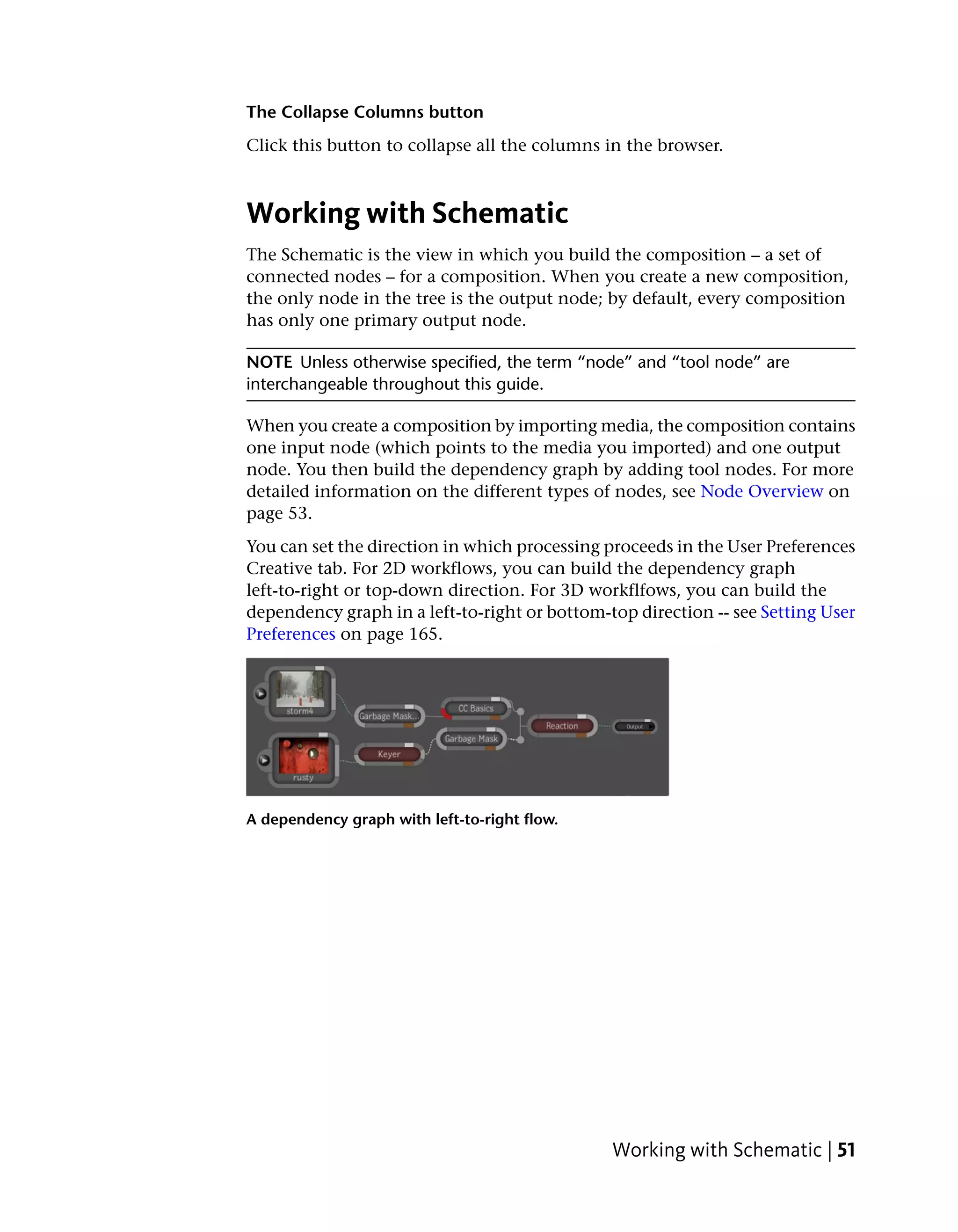
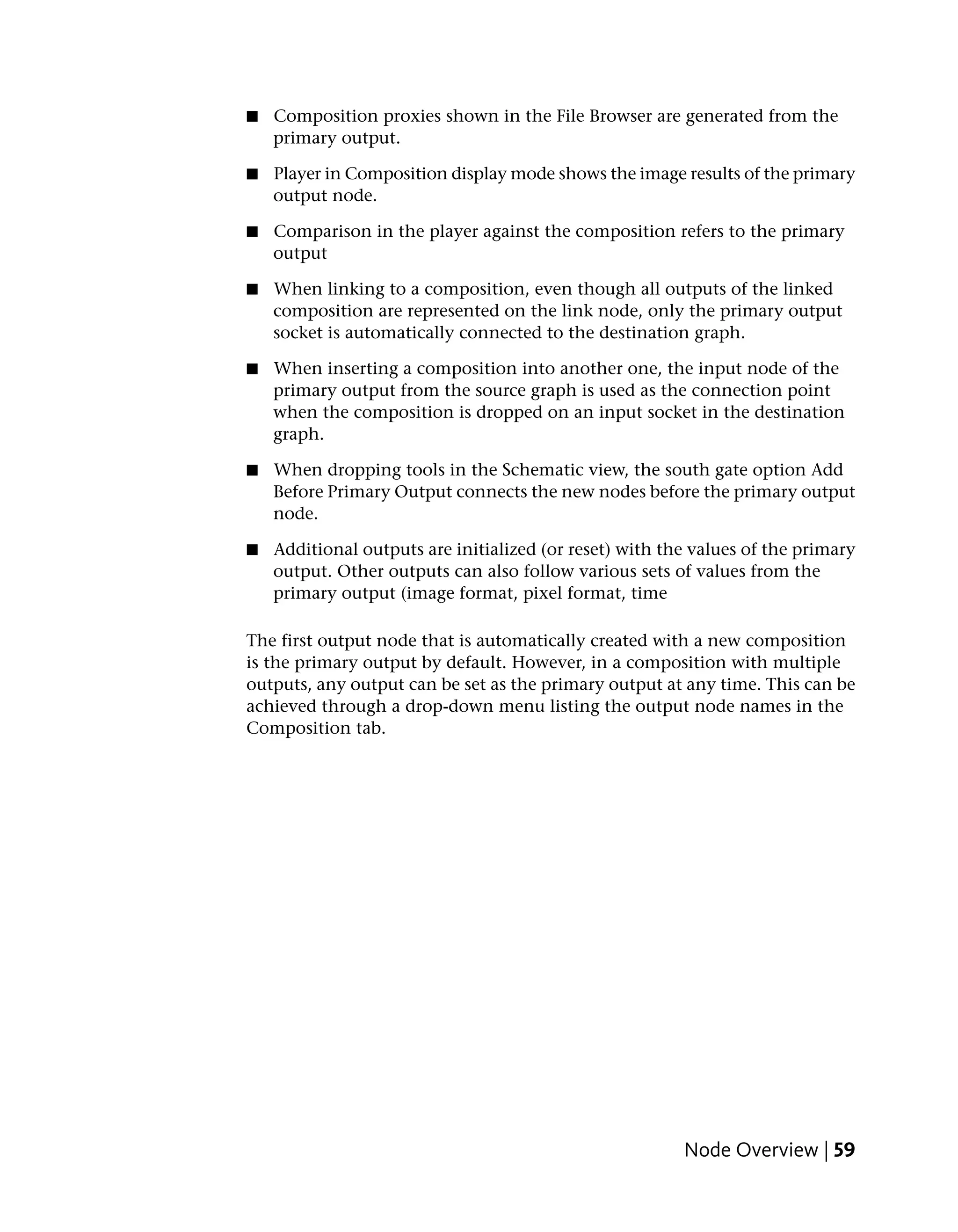
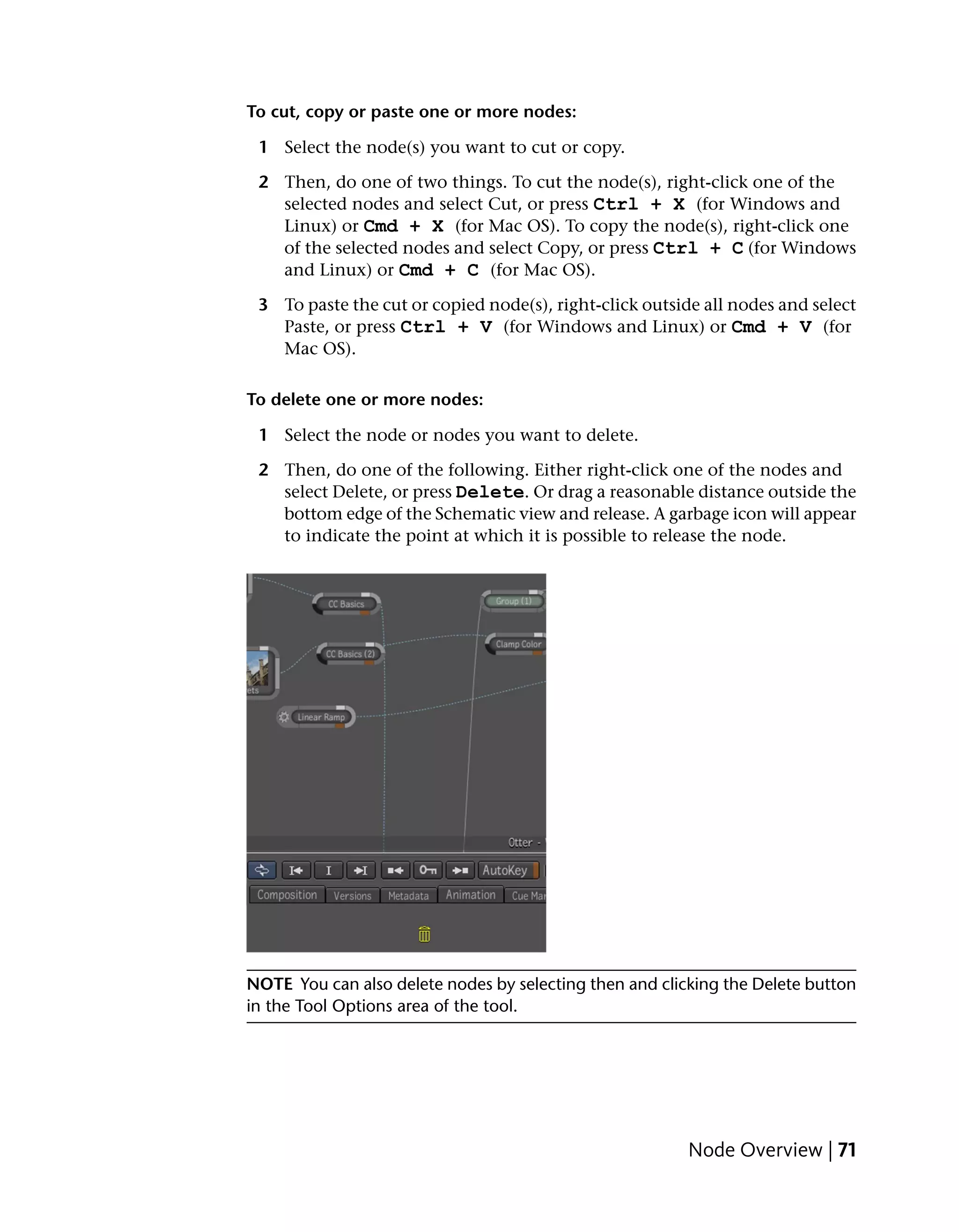
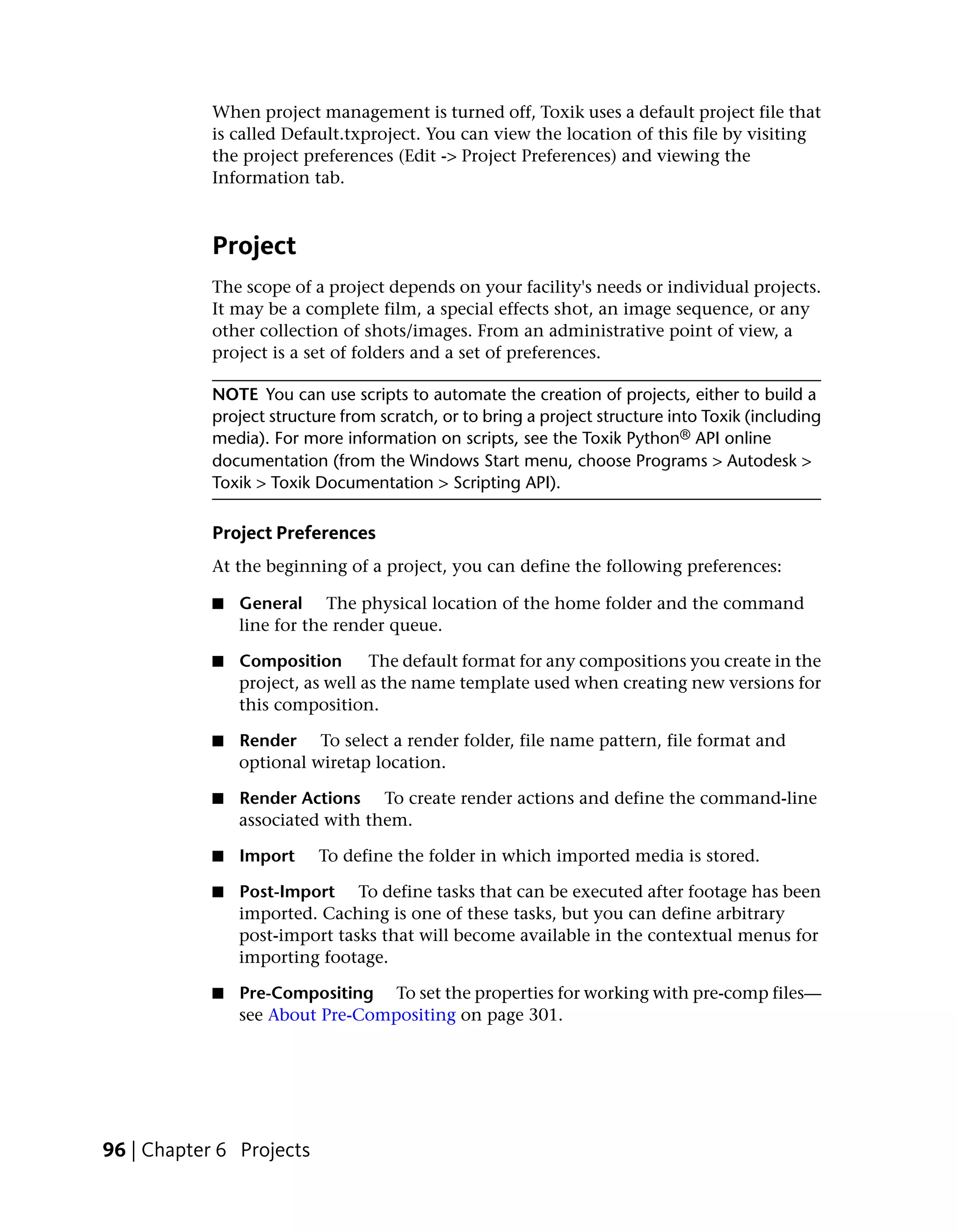
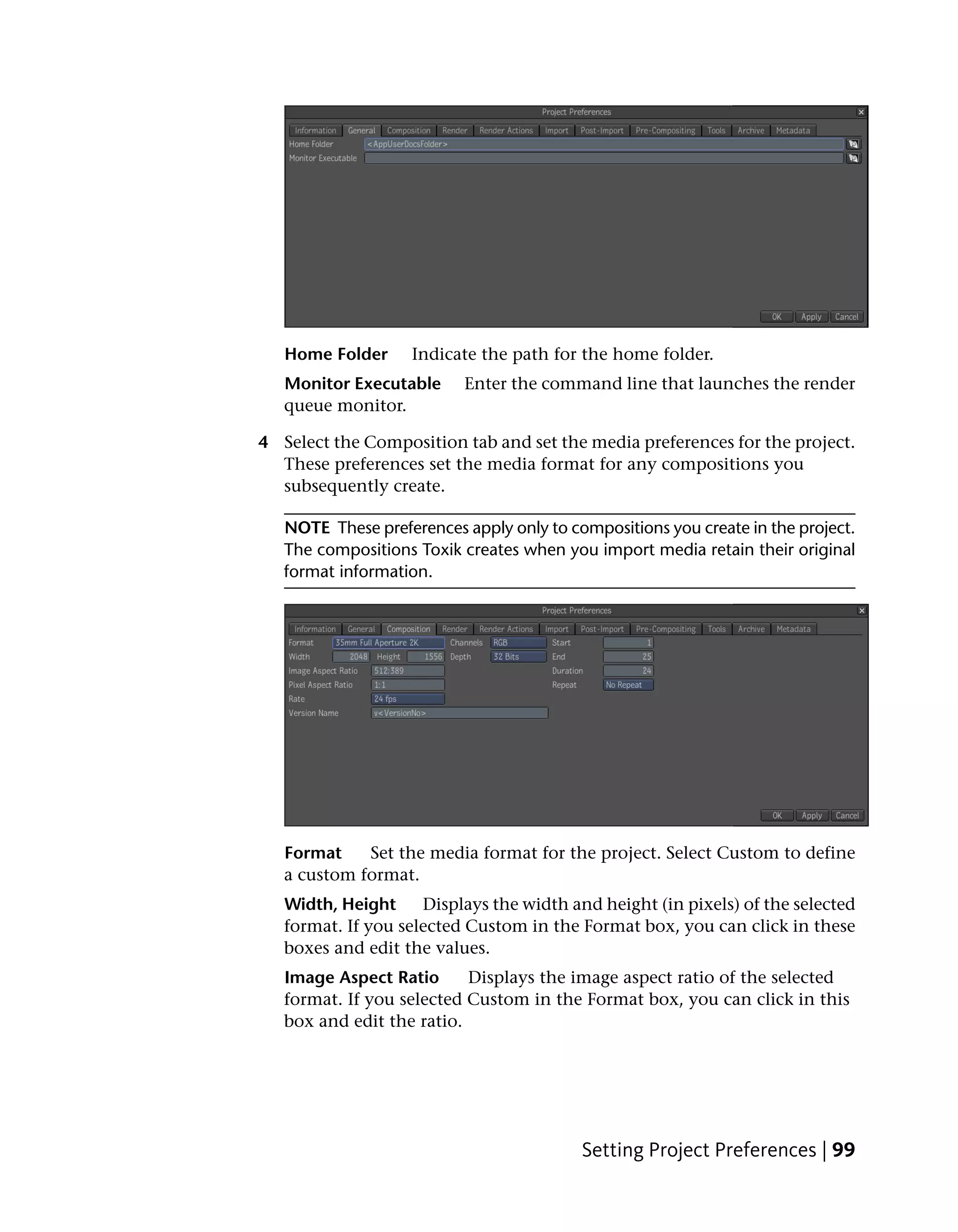
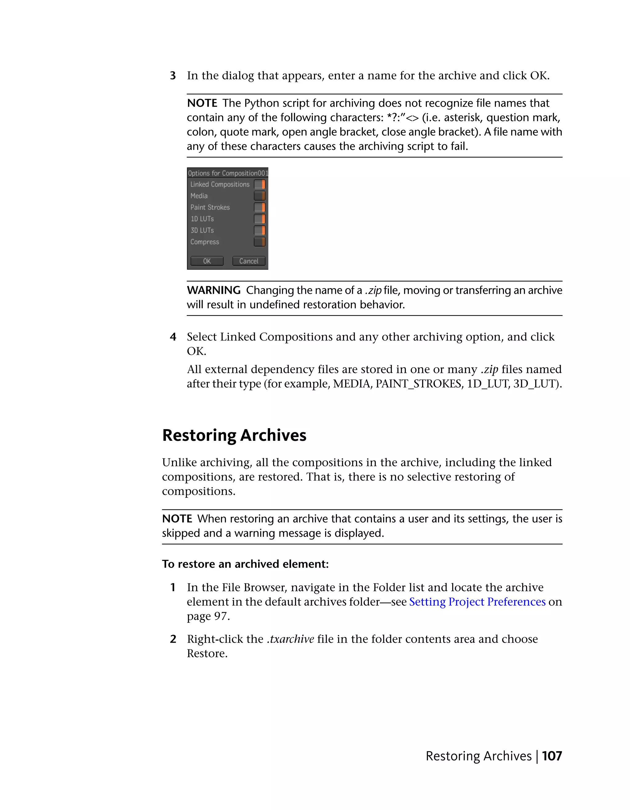
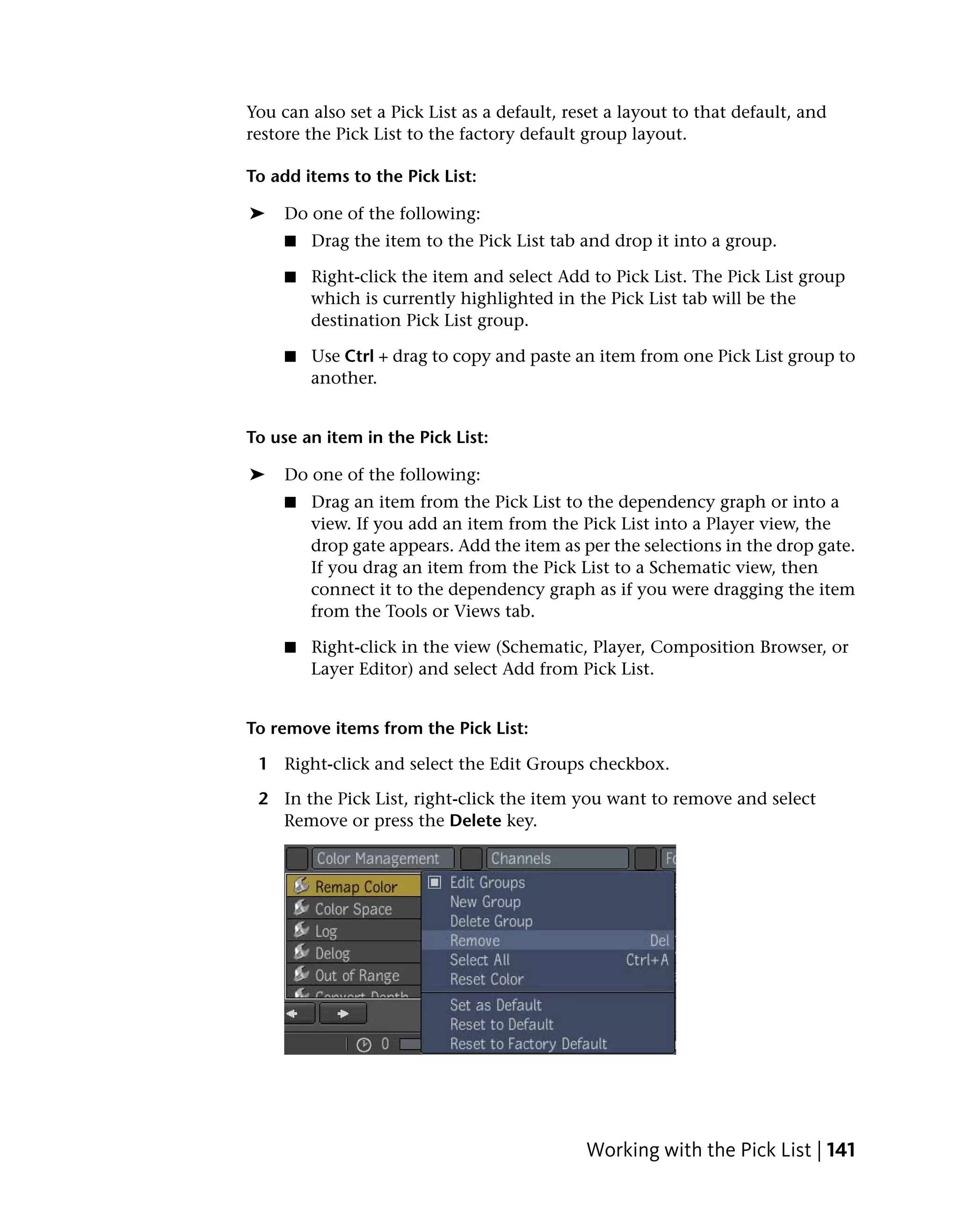
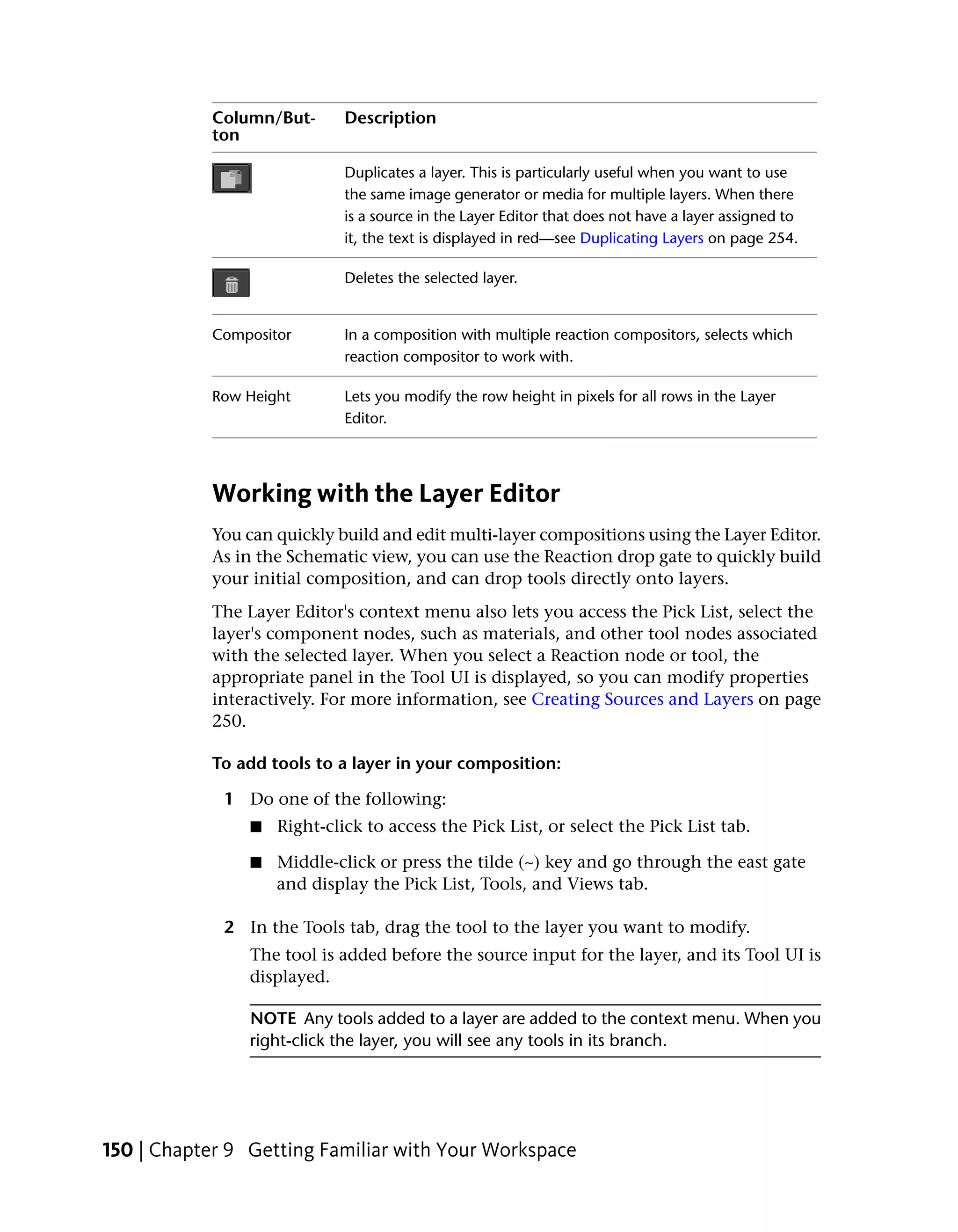
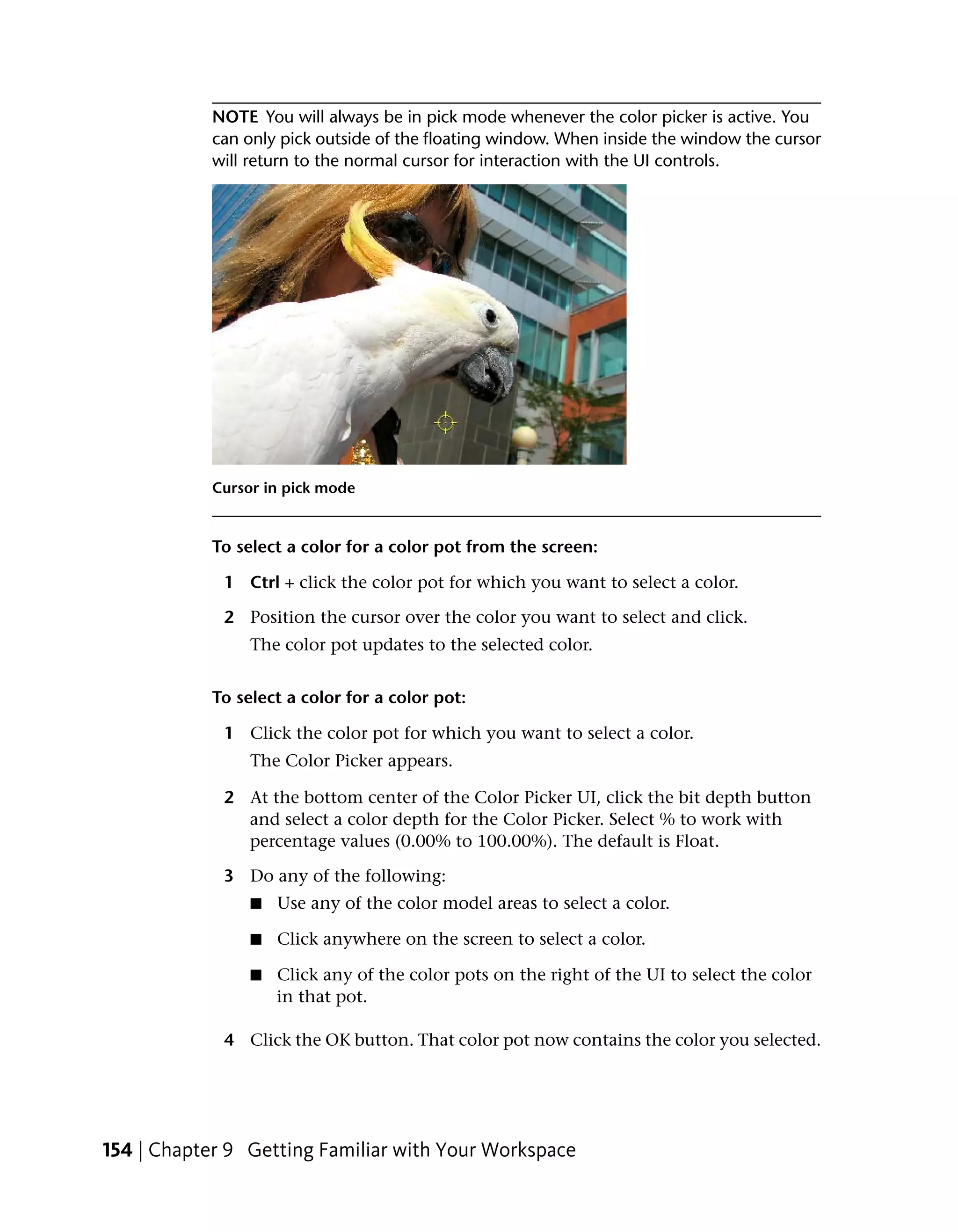
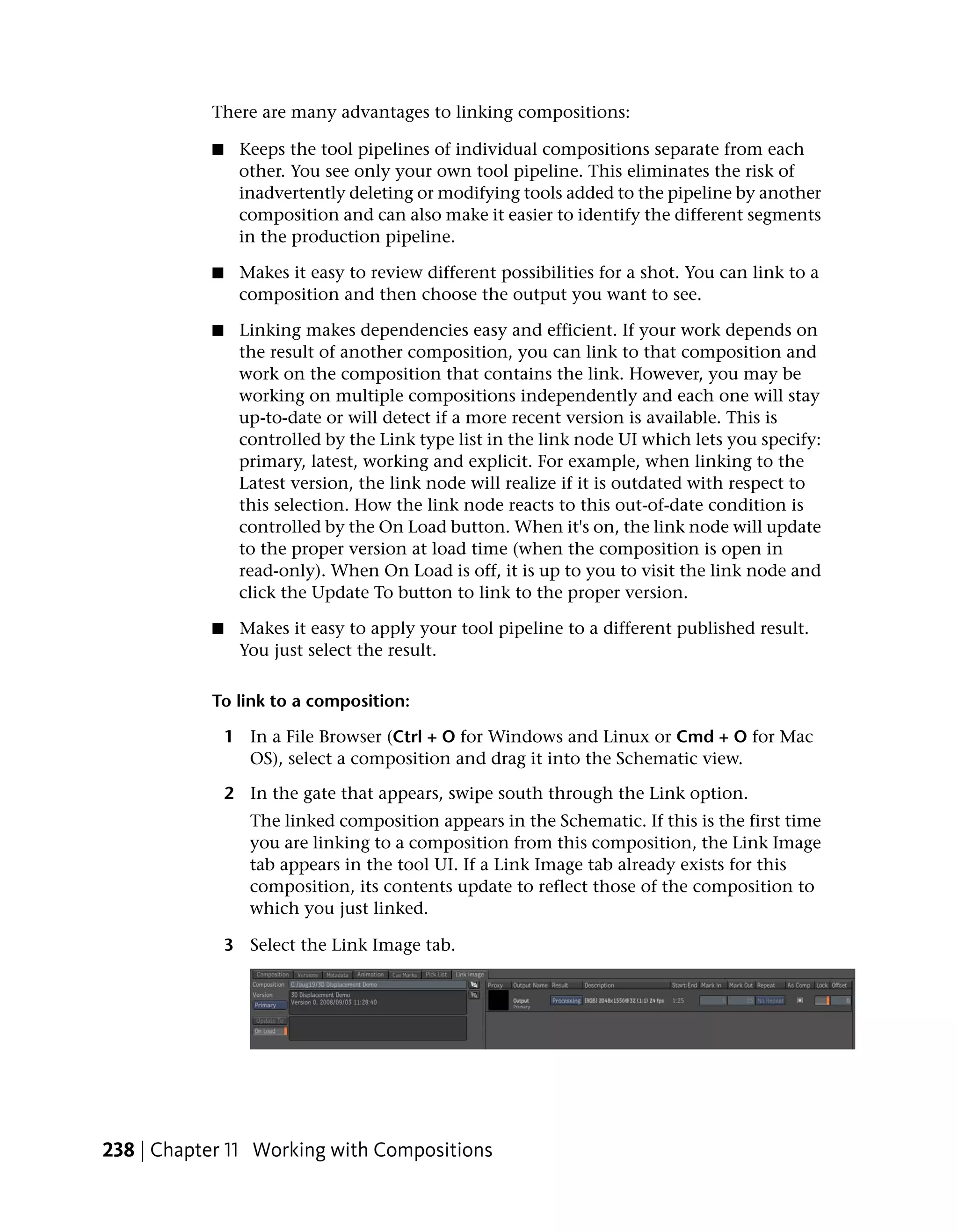
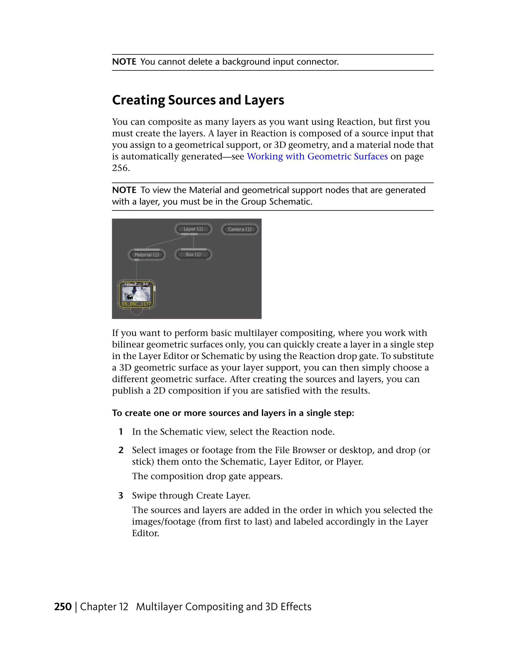
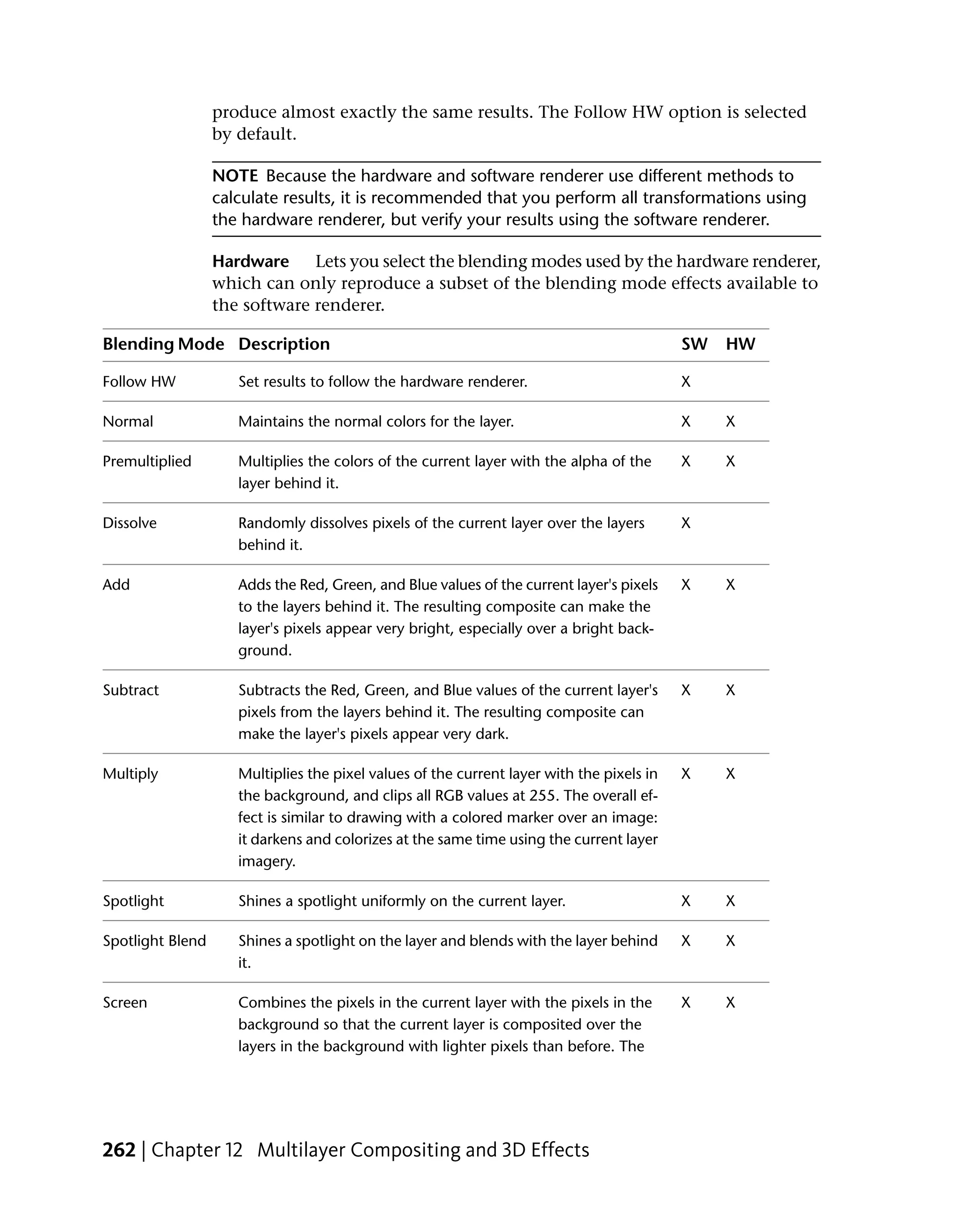
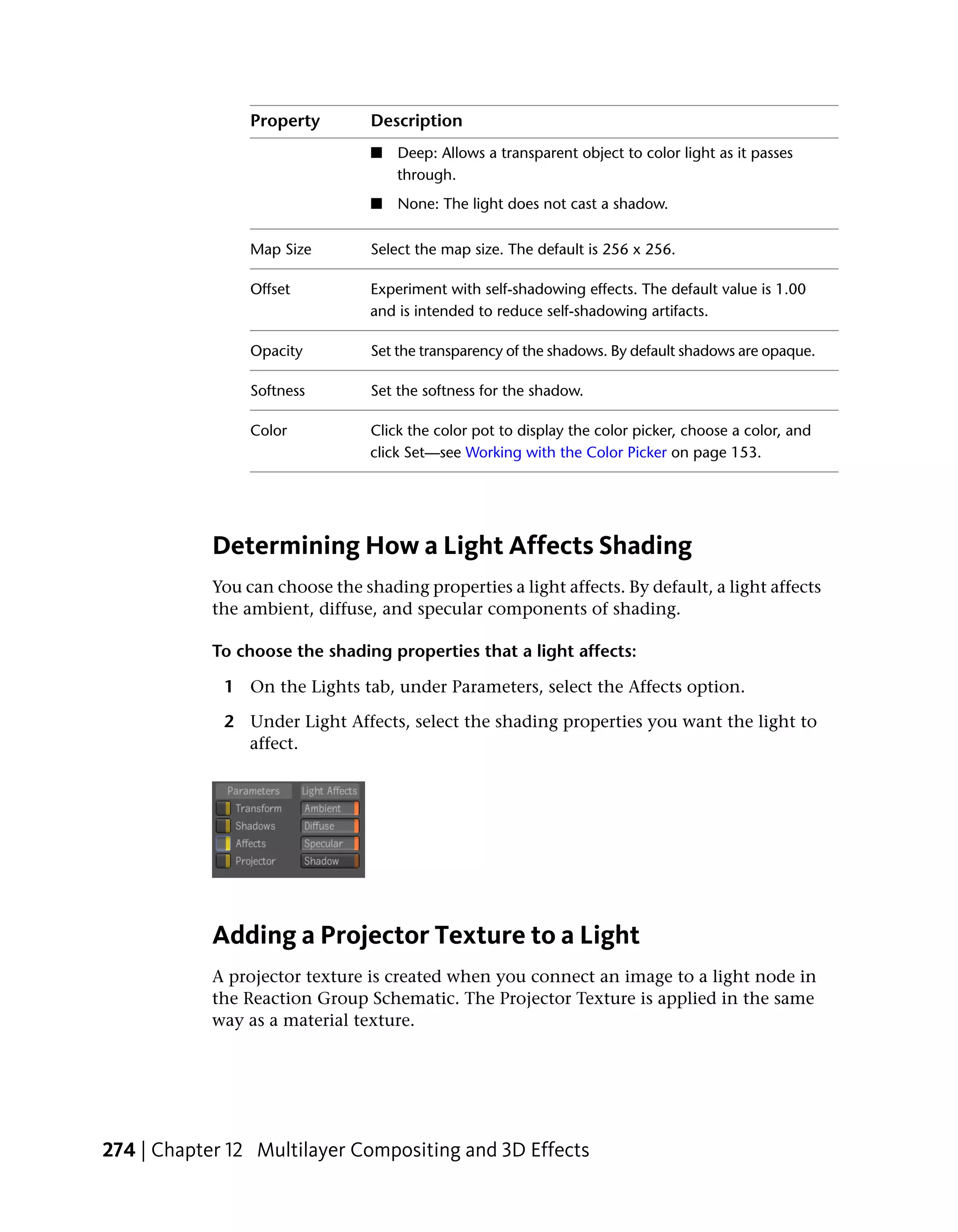
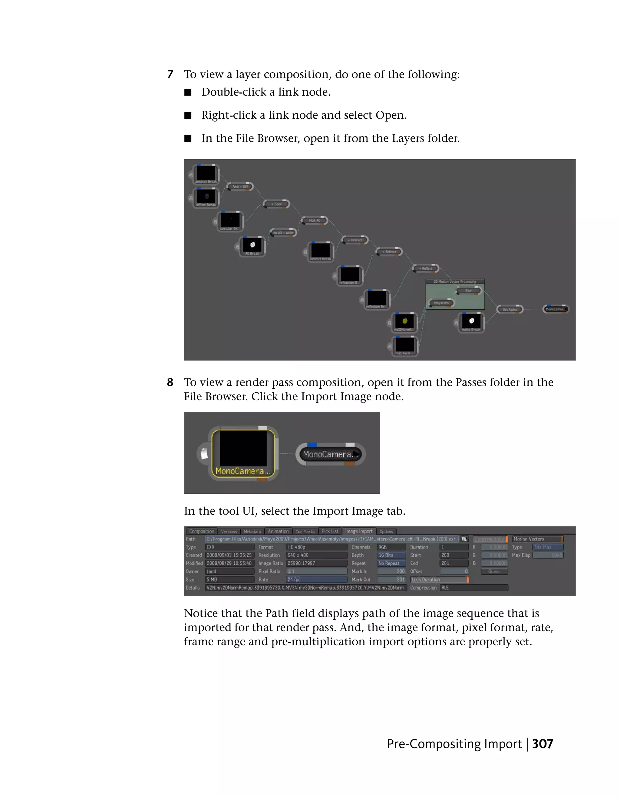
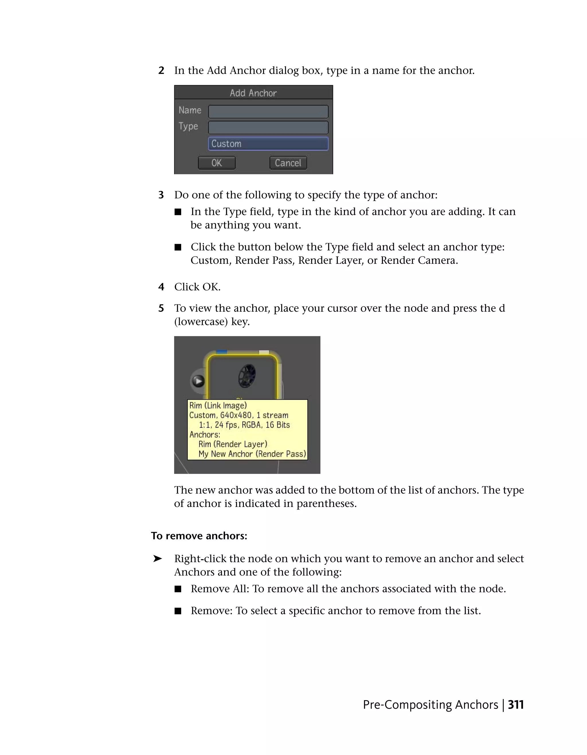
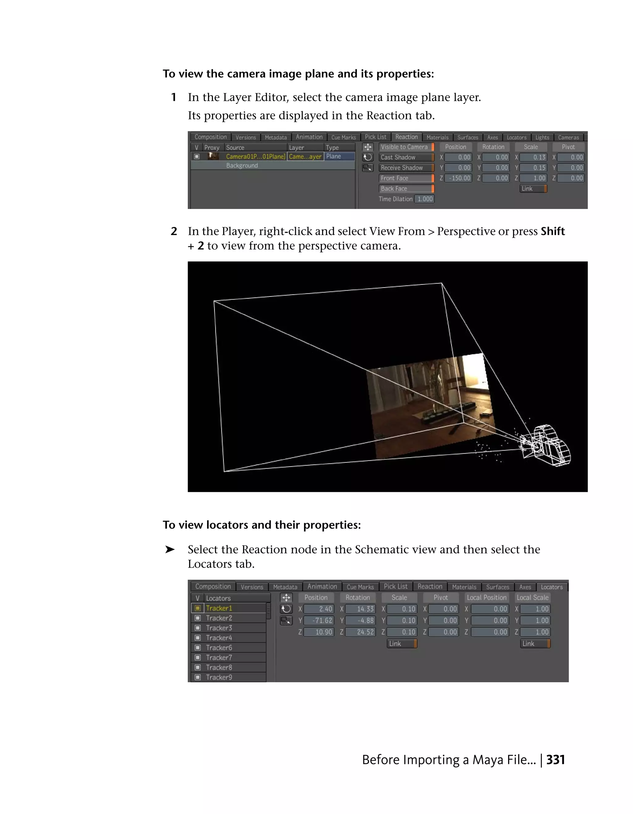
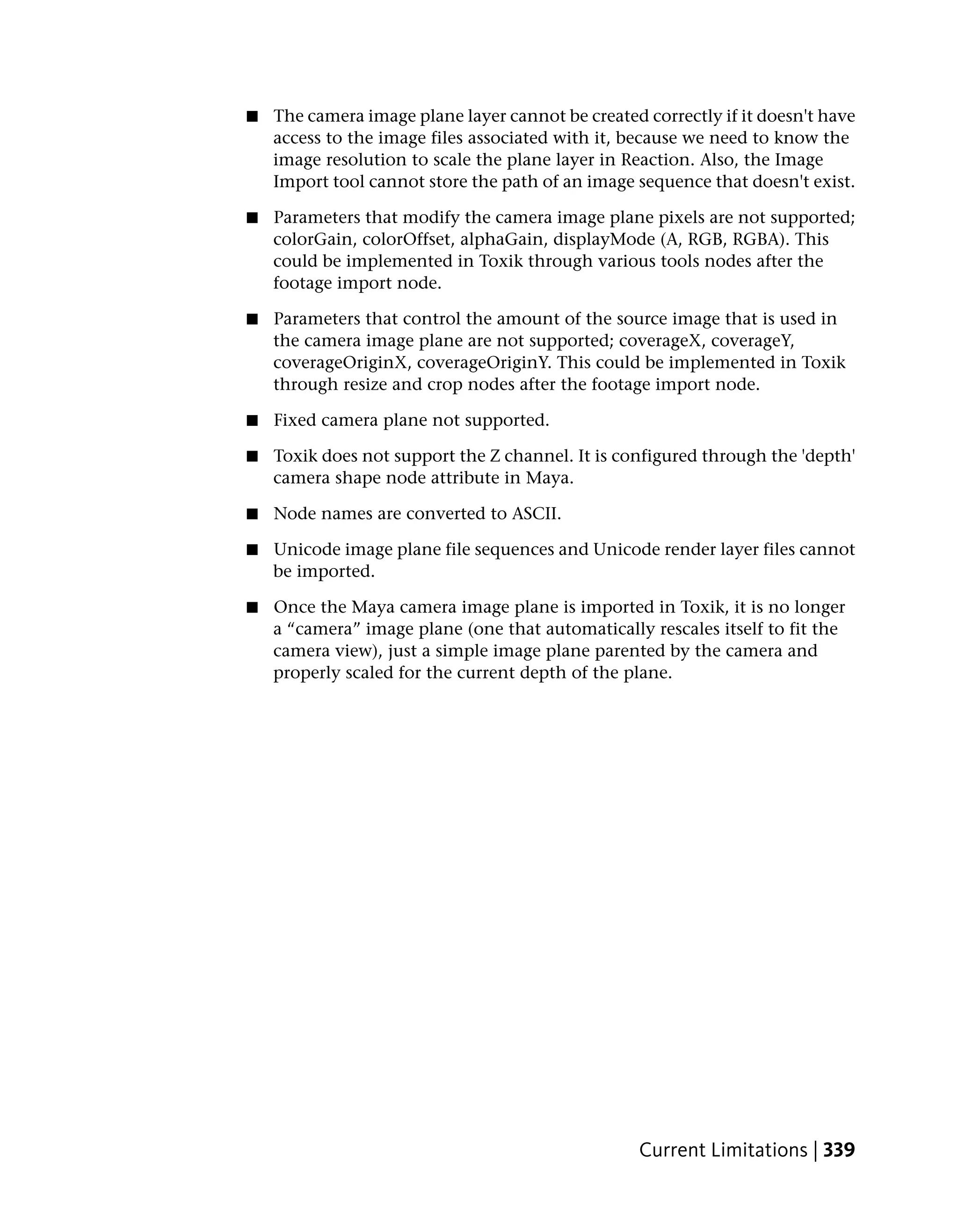
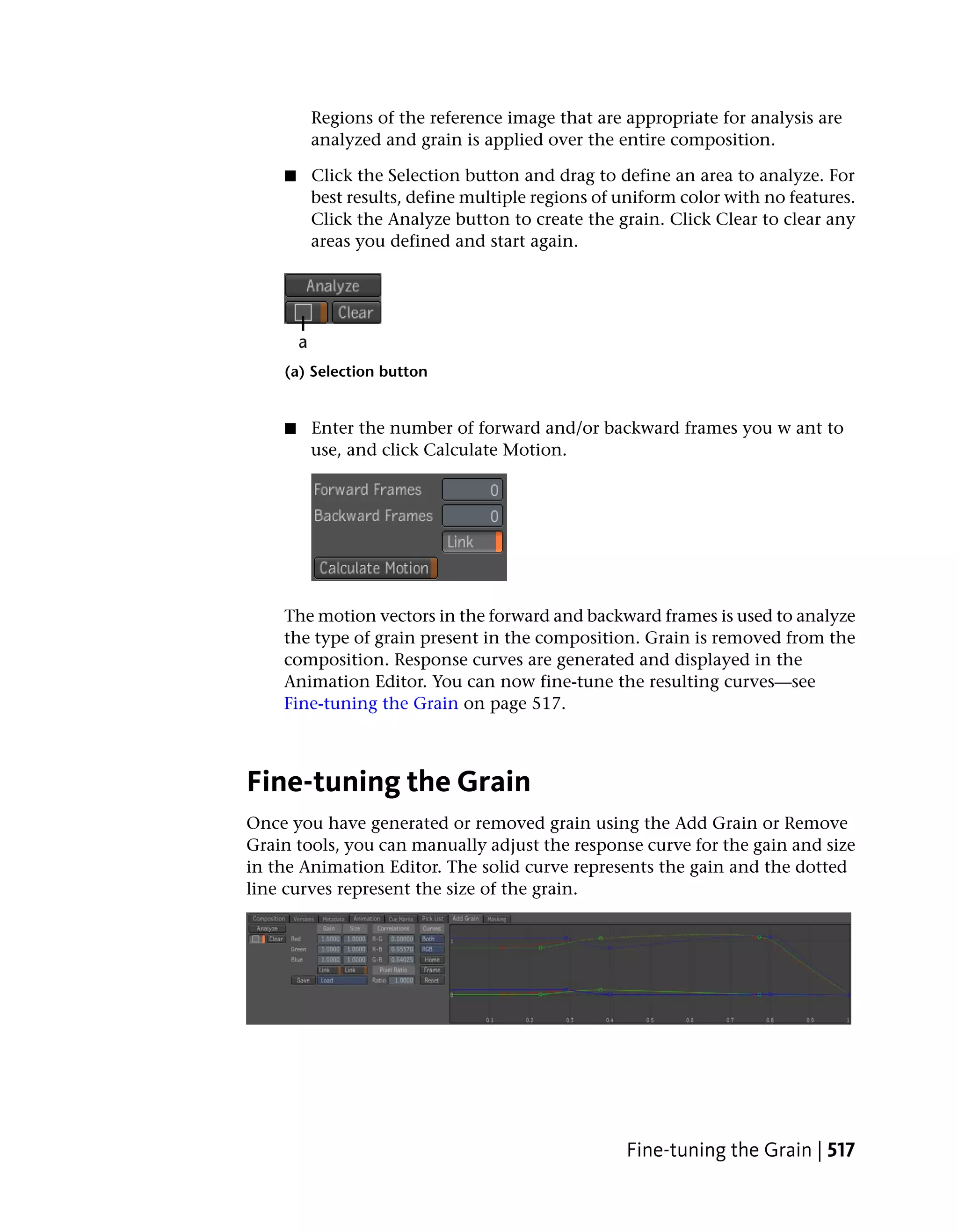
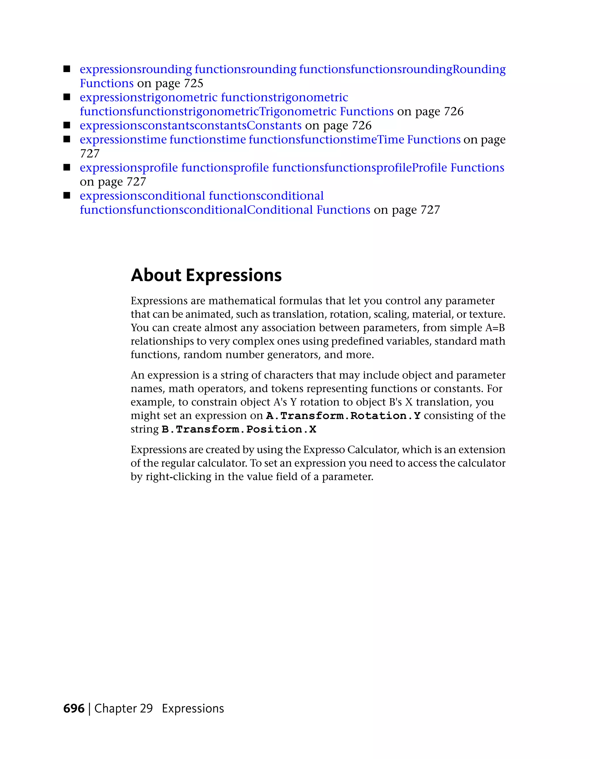
![The Blur Alpha tool has the following parameters:
■ X Radius Change this value to blur horizontal pixels.
■ Y Radius Change this value to blur vertical pixels.
■ Link Select to link X and Y values.
NOTE X and Y Radius are animatable attributes—see Marking Attributes for
Keyframing on page 664.
Clamp Alpha
The Clamp Alpha tool is used to bring the alpha channel of the primary input
within a predetermined range. You can use clamp alpha values outside of the
[0,1] range in order to prepare the alpha channel for use in compositing
operators. This is necessary because Toxik does not force alpha values to be
in the [0,1] range.
The Clamp Alpha tool contains the following parameters:
■ Minimum Alpha Set Largest negative float point. By default, Min is 0.
■ Maximum Alpha Set Largest positive float point. By default Max is 1.0.
NOTE Min and Max Alpha are animatable attributes—see Marking Attributes for
Keyframing on page 664.
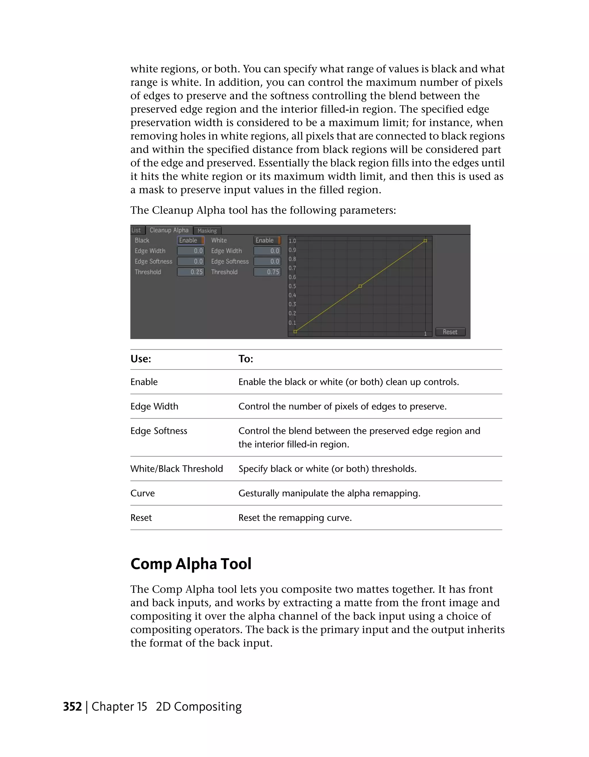
Cleanup Alpha
The Cleanup Alpha tool lets you remove gray details from white and/or black
regions of the alpha channel. You can choose to remove holes in black regions,
Clamp Alpha | 351](https://image.slidesharecdn.com/mayacompositeuserguide-1260452105-phpapp01/75/Mayacompositeuserguide-367-2048.jpg)
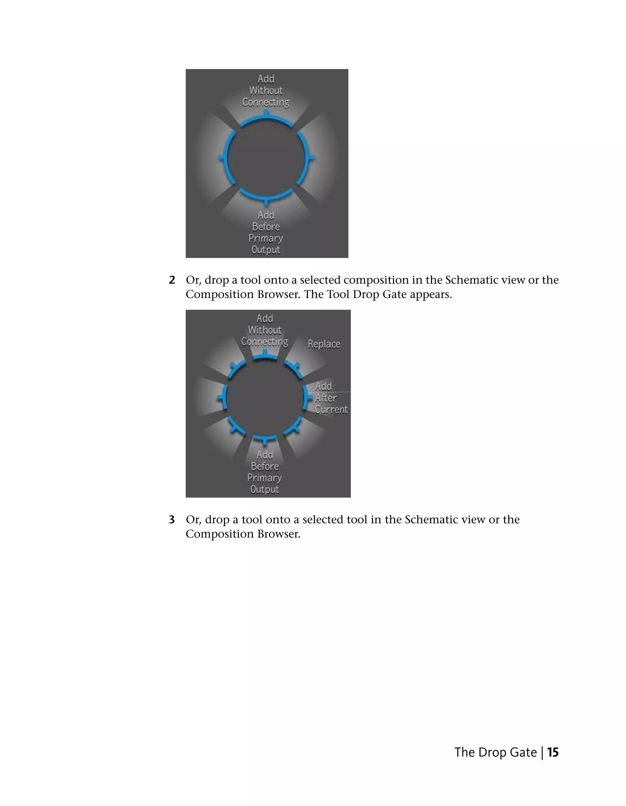
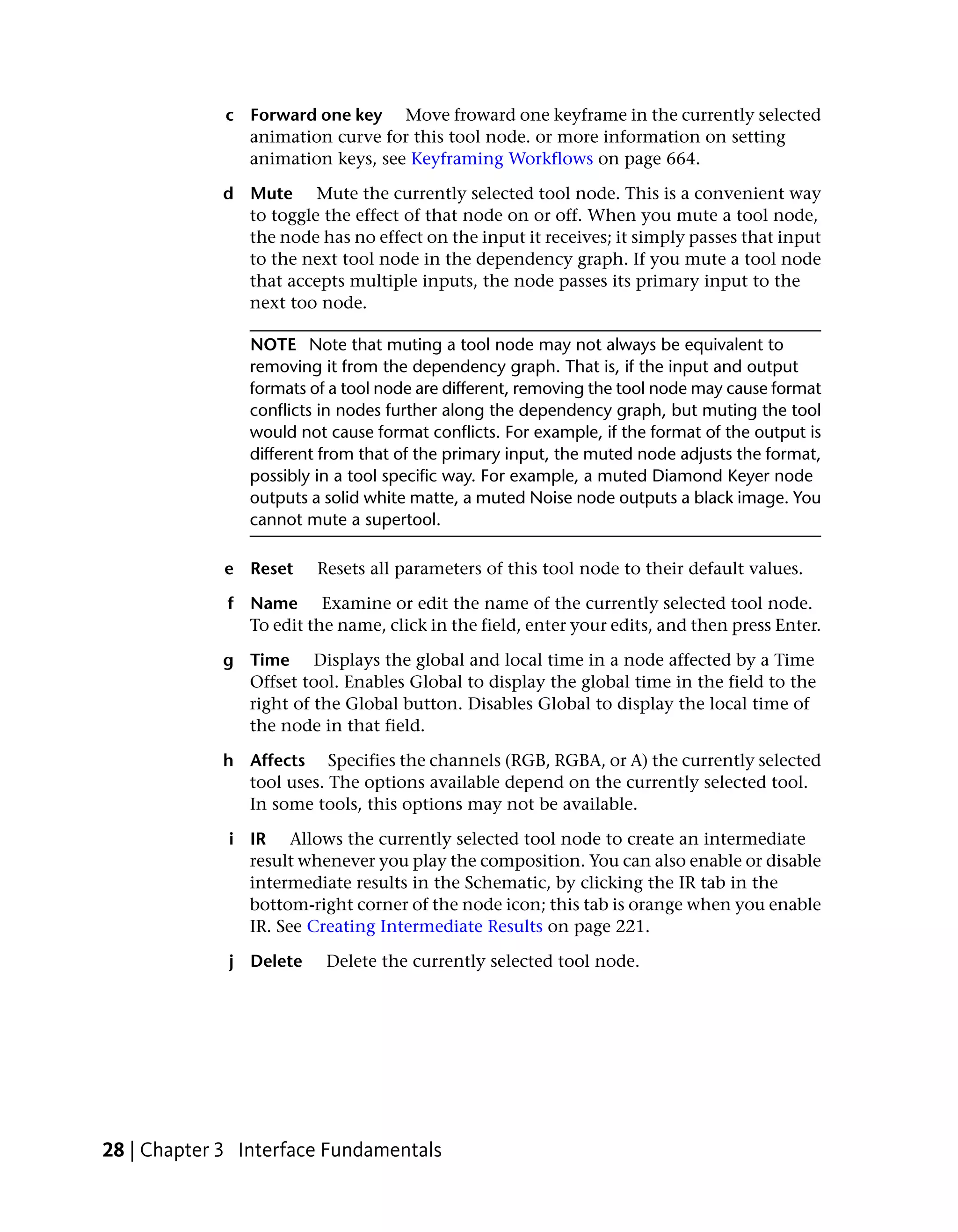
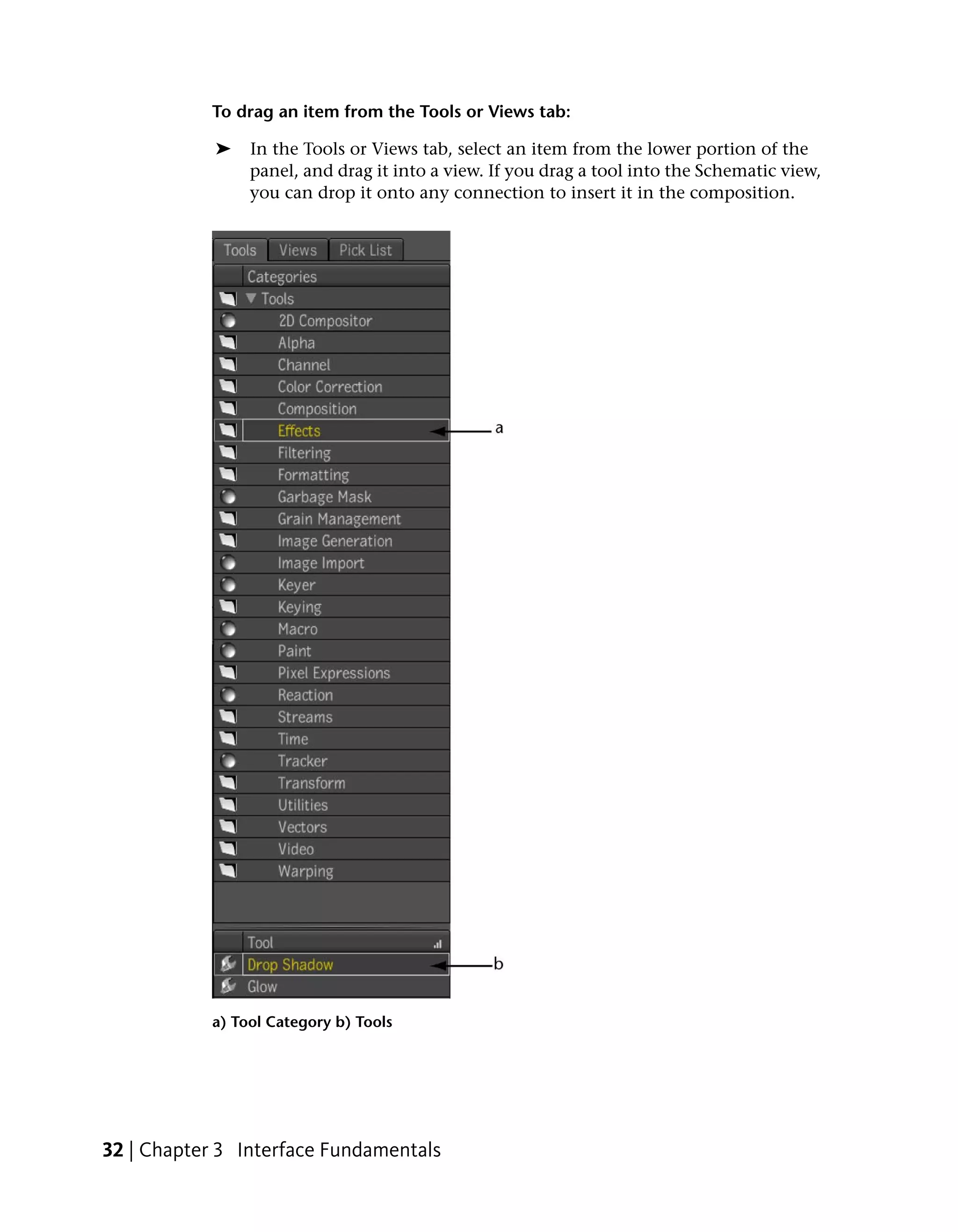
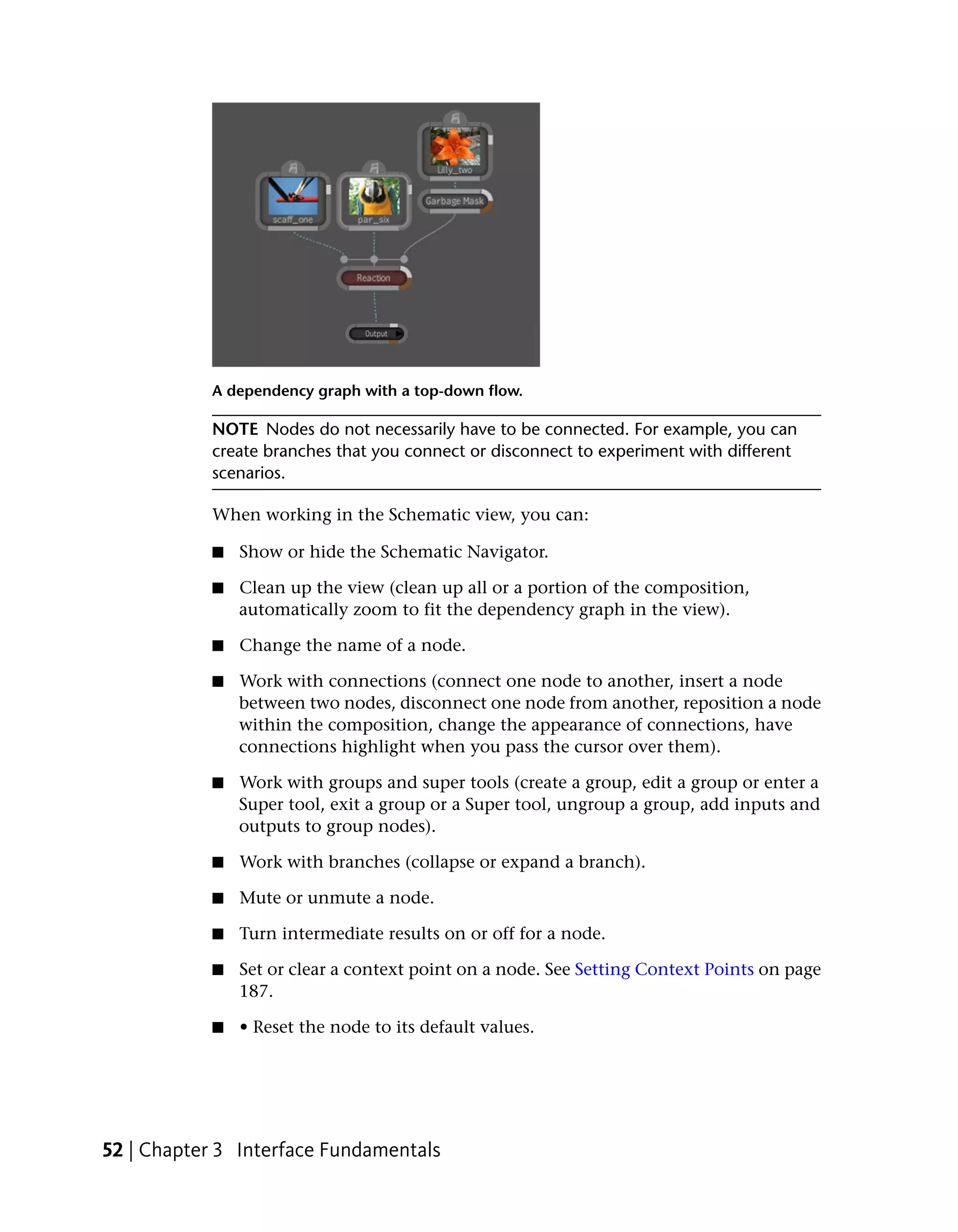
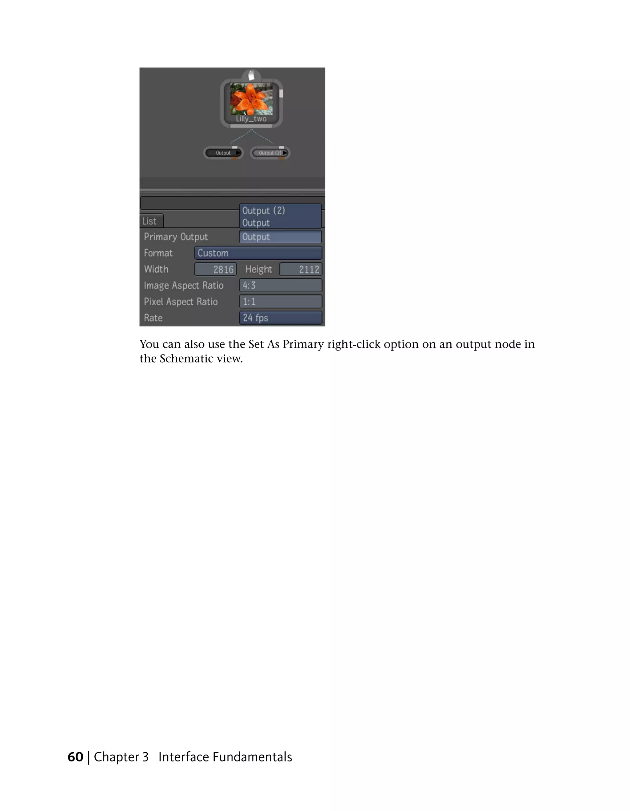
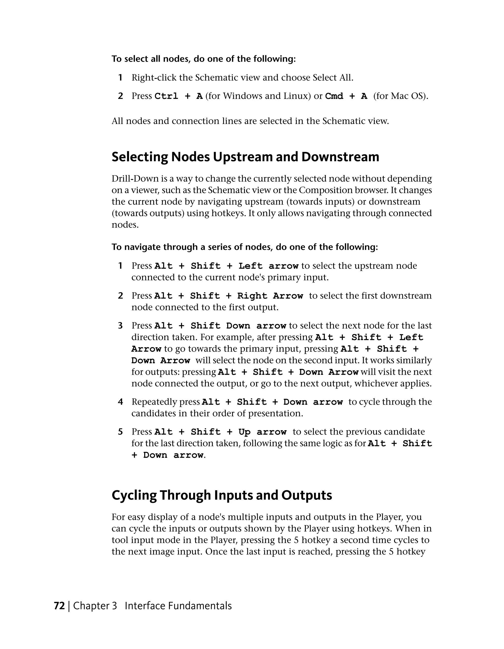
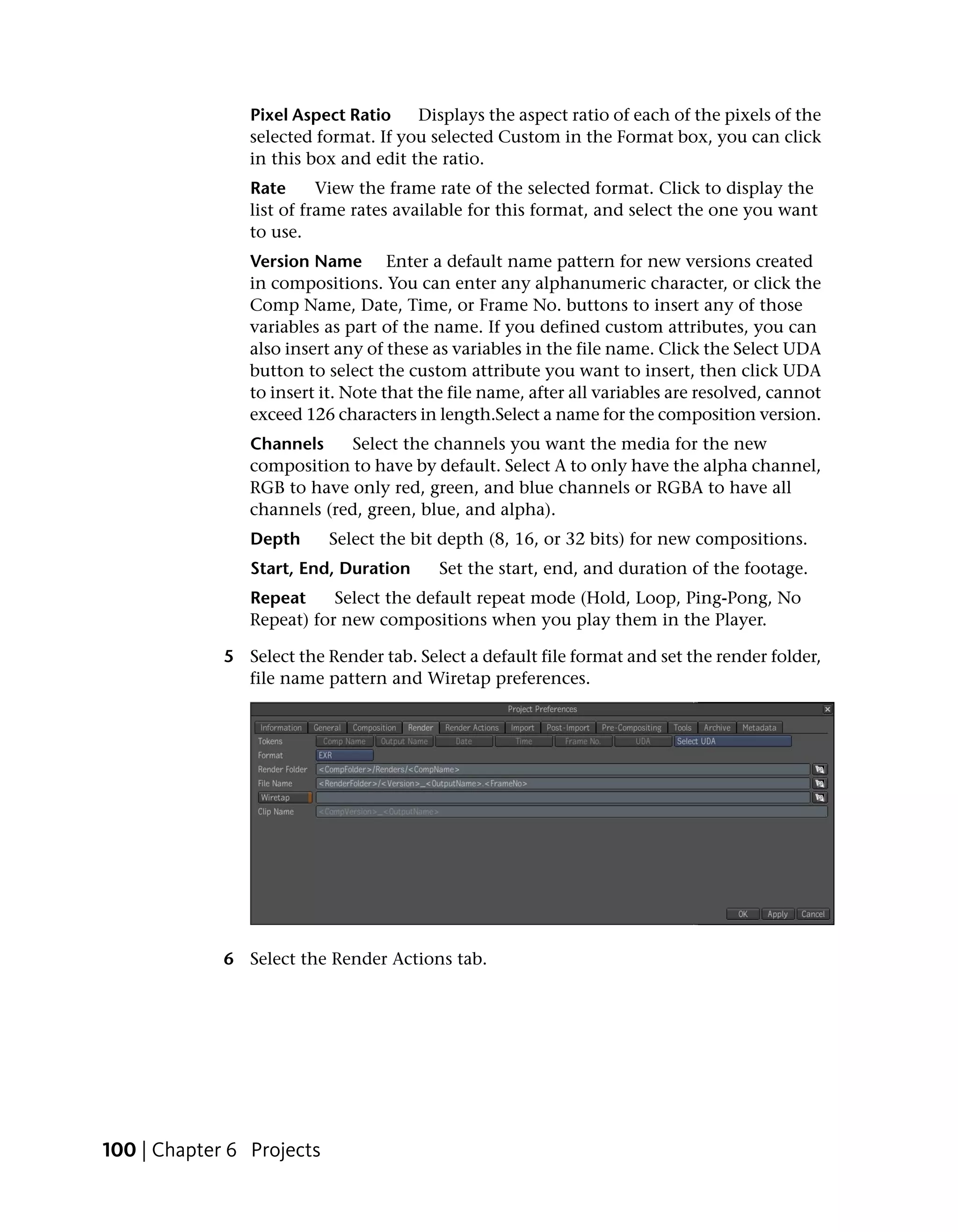
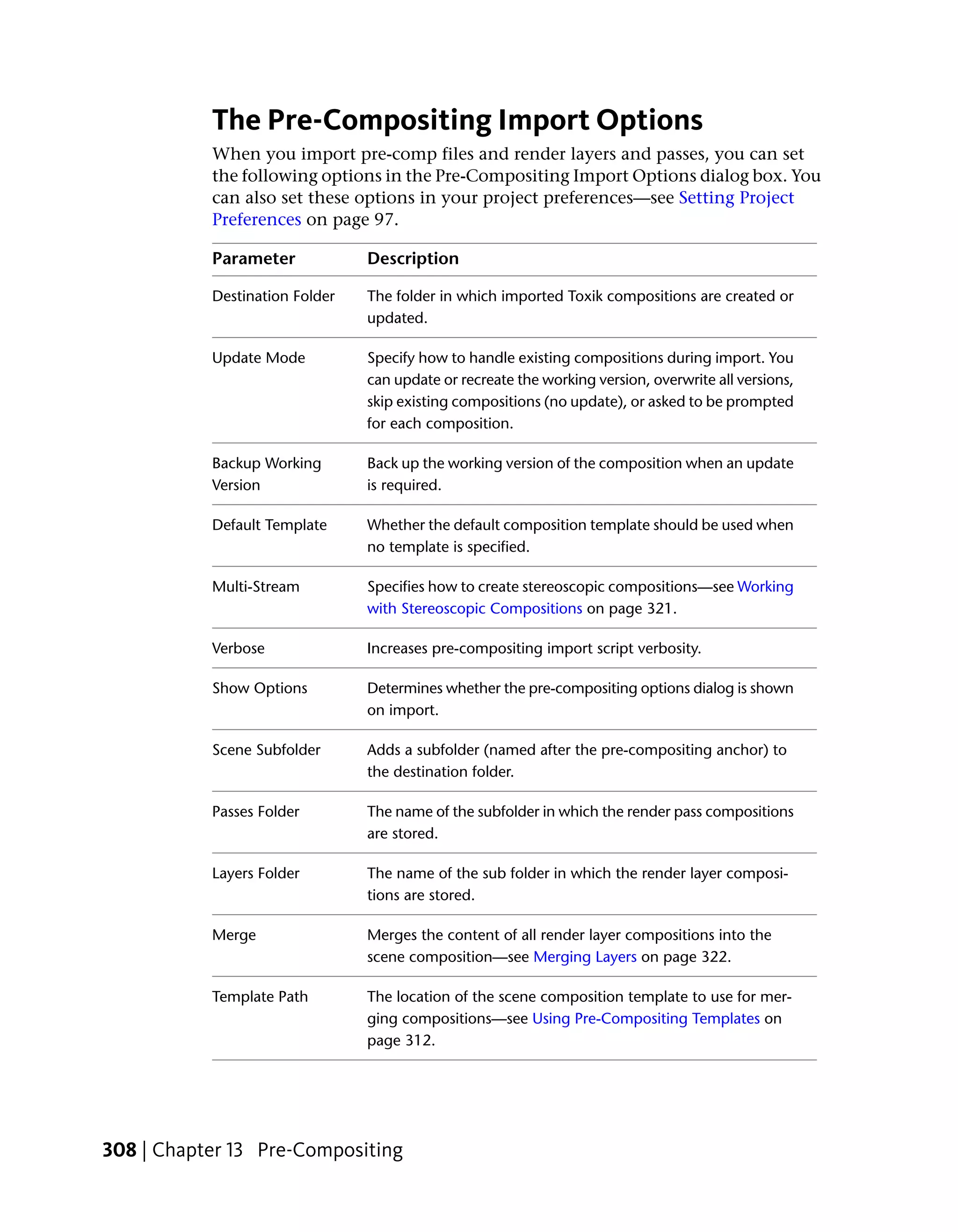
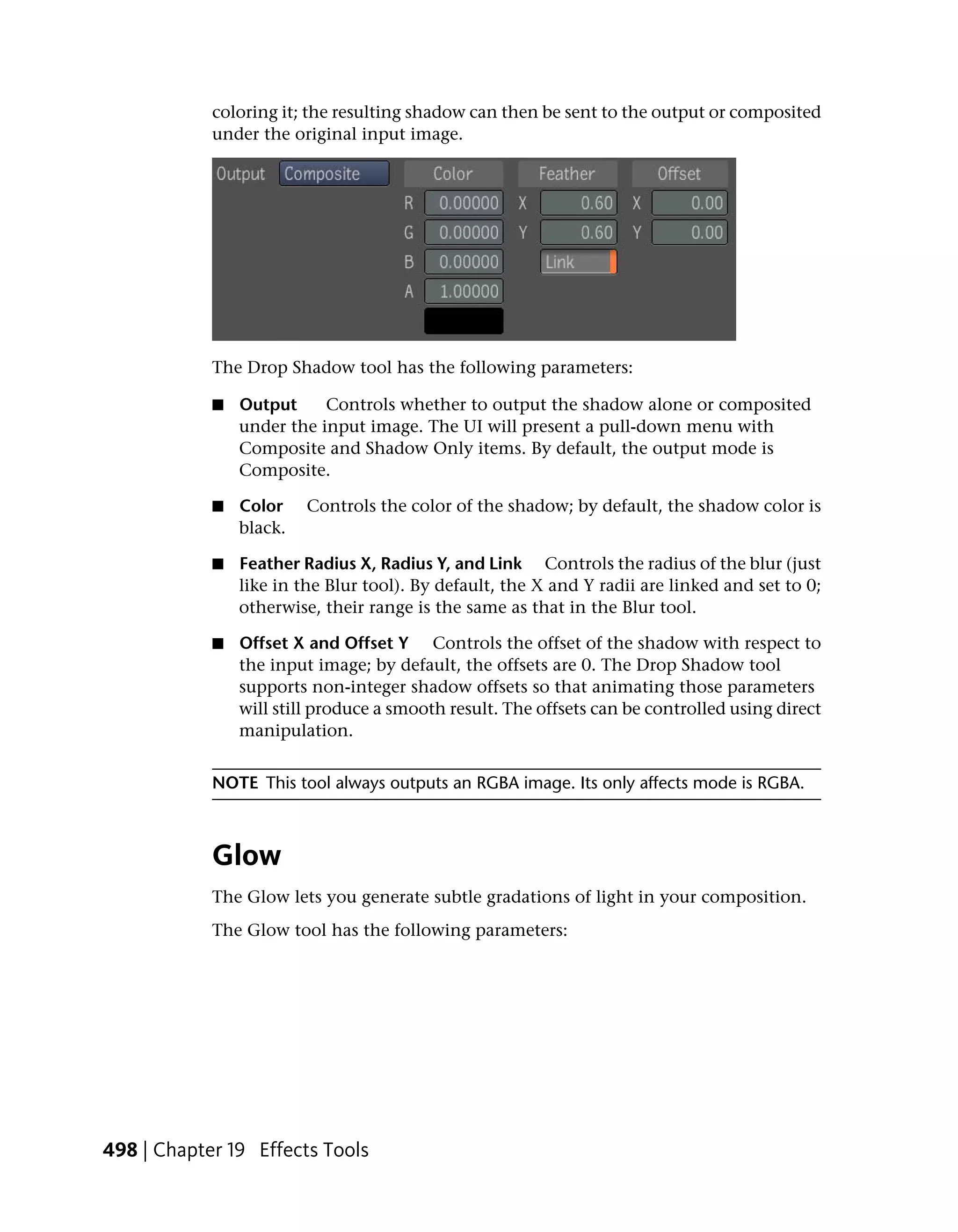
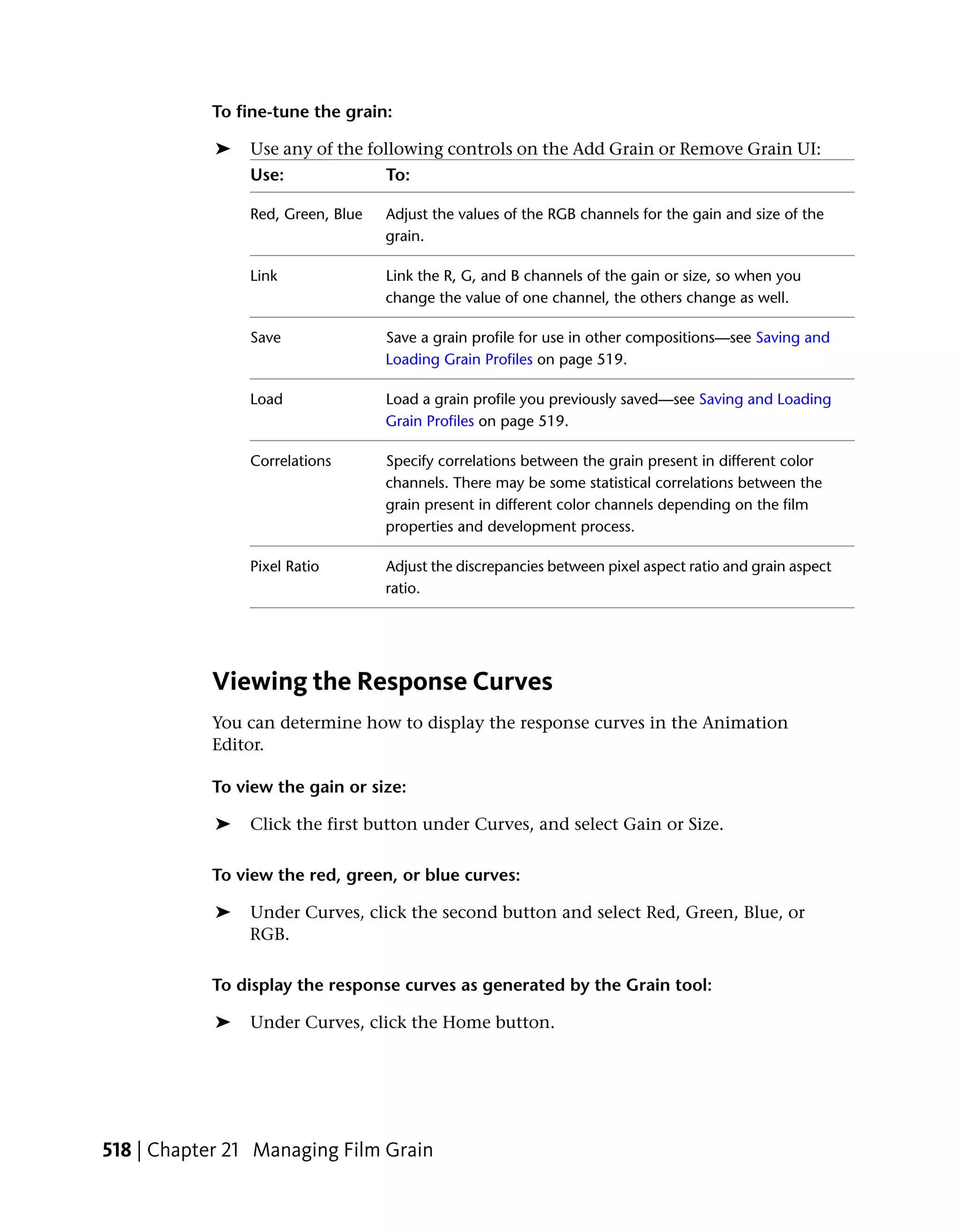
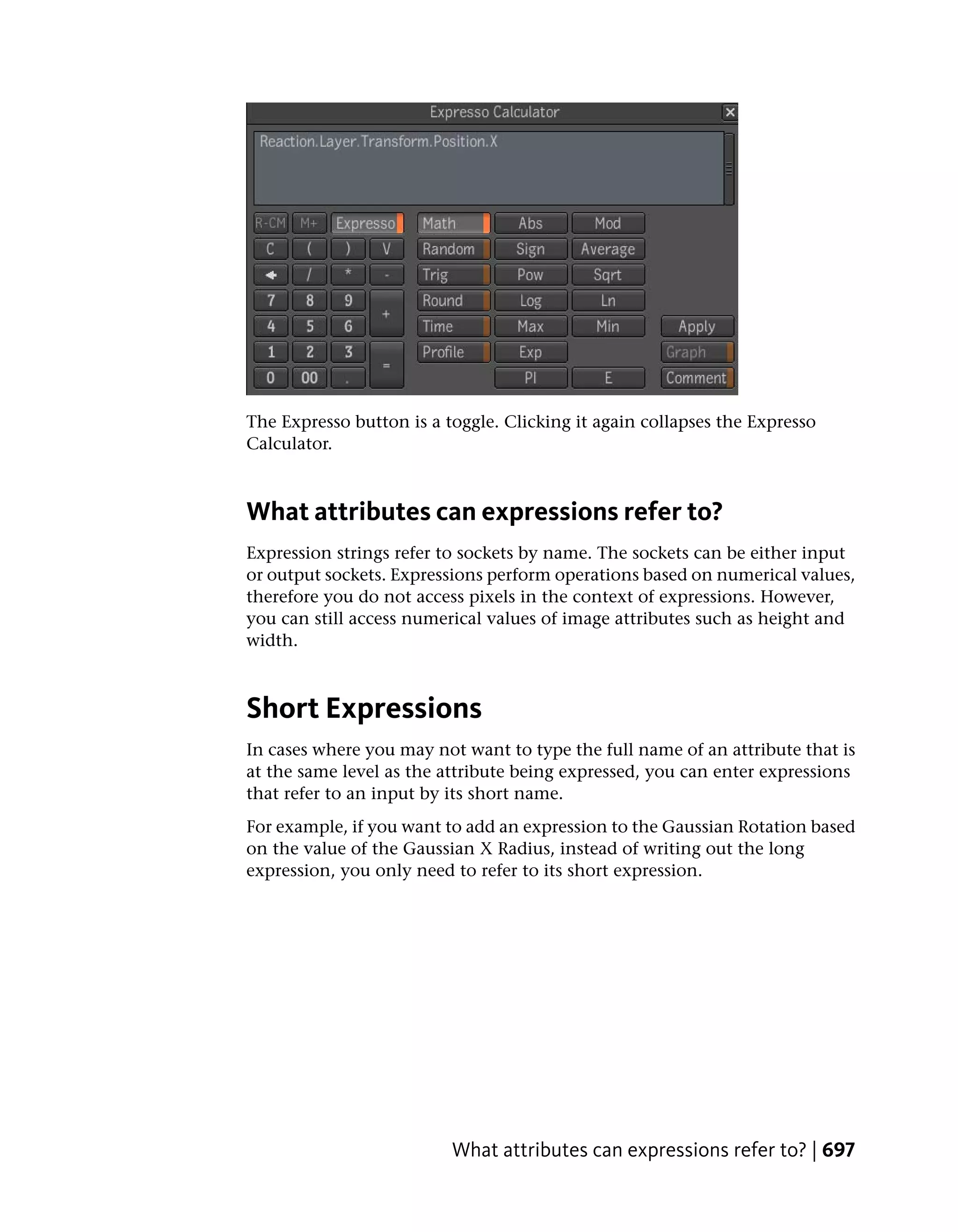
![This tool only affects alpha. If the back is an RGBA image, the color part is
simply copied to the output.
NOTE The alpha output of this tool is always clamped to the [0,1] interval.
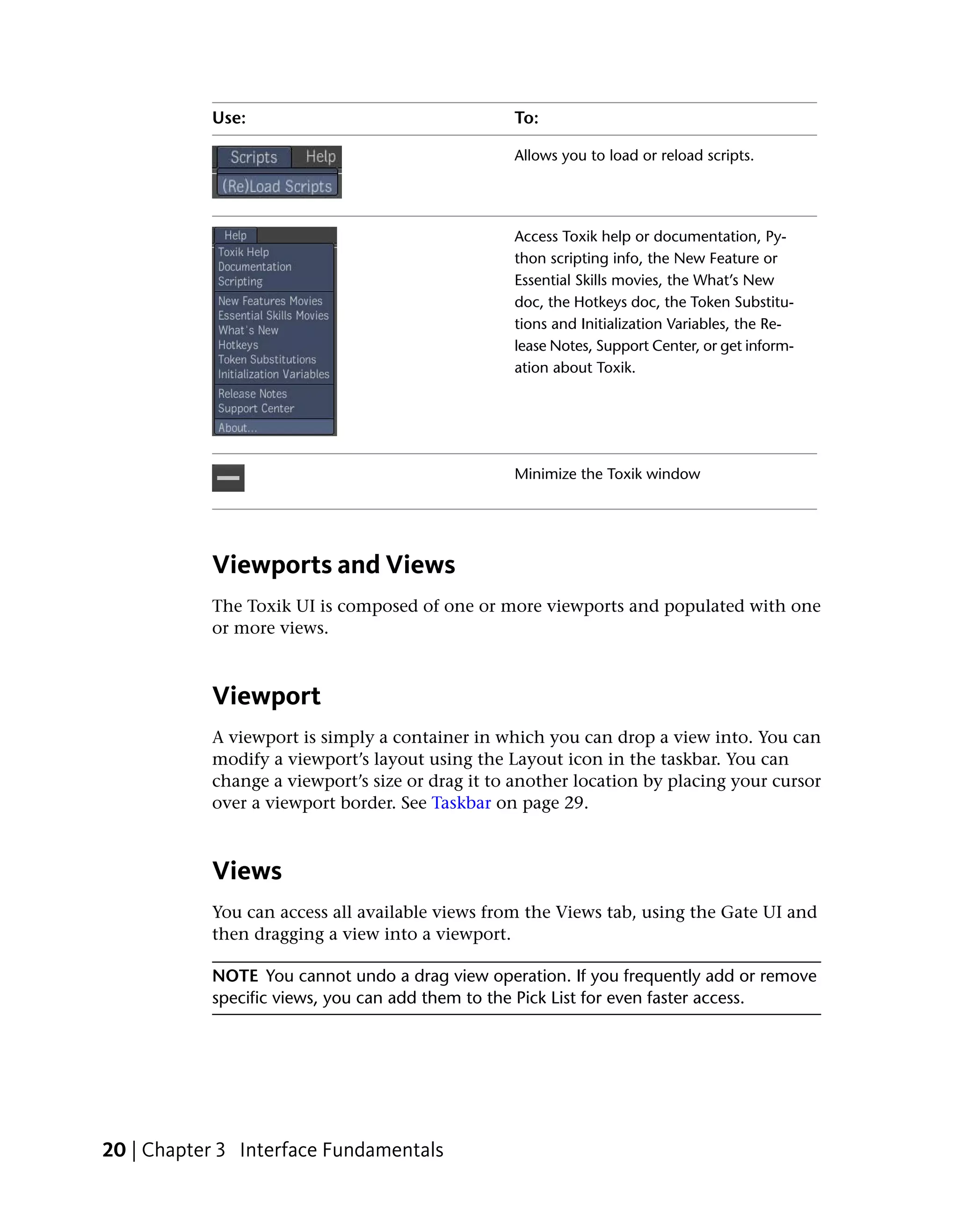
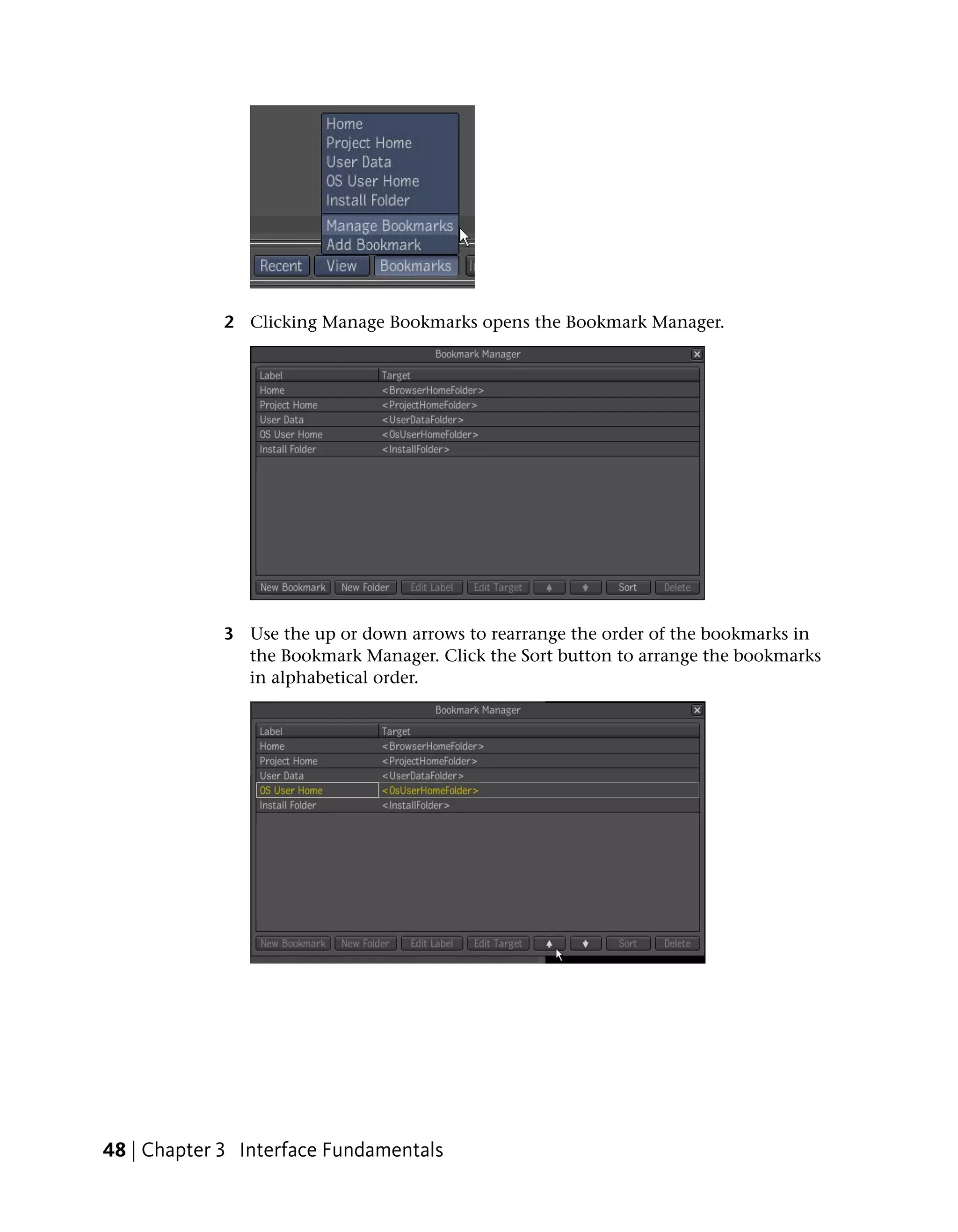
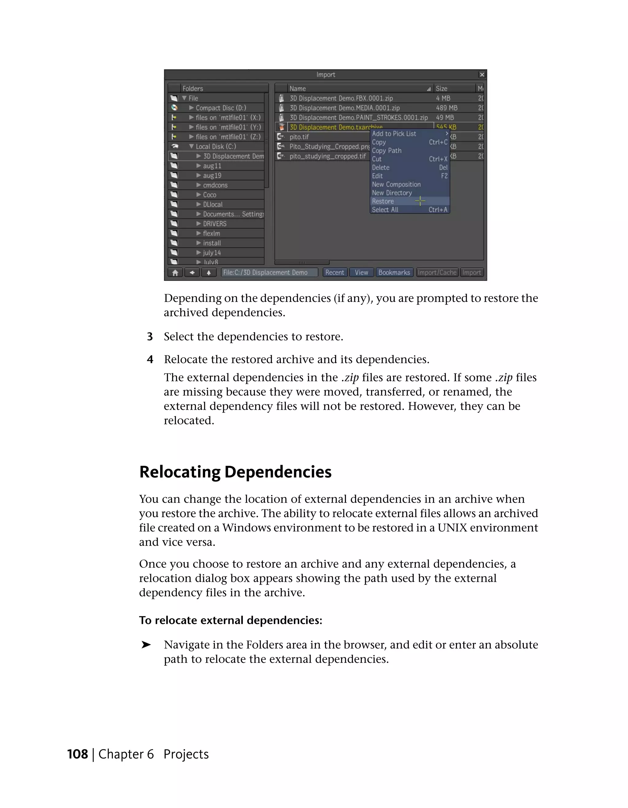
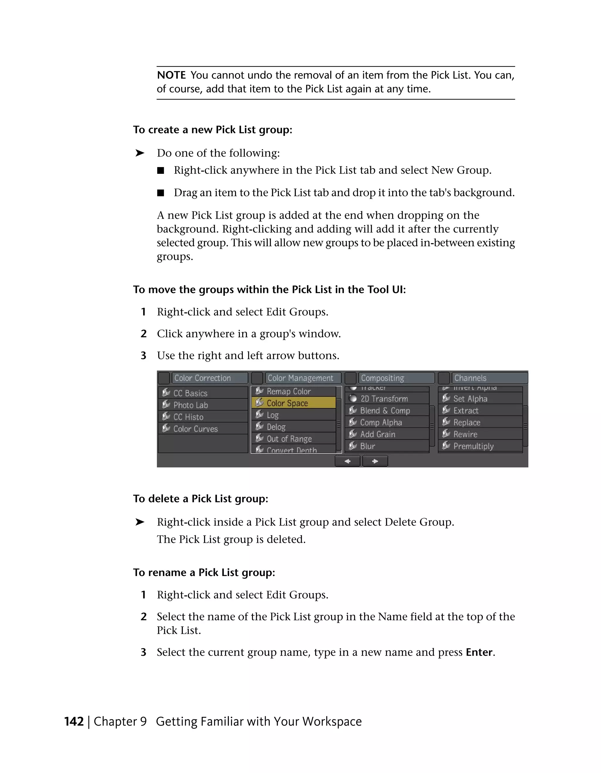
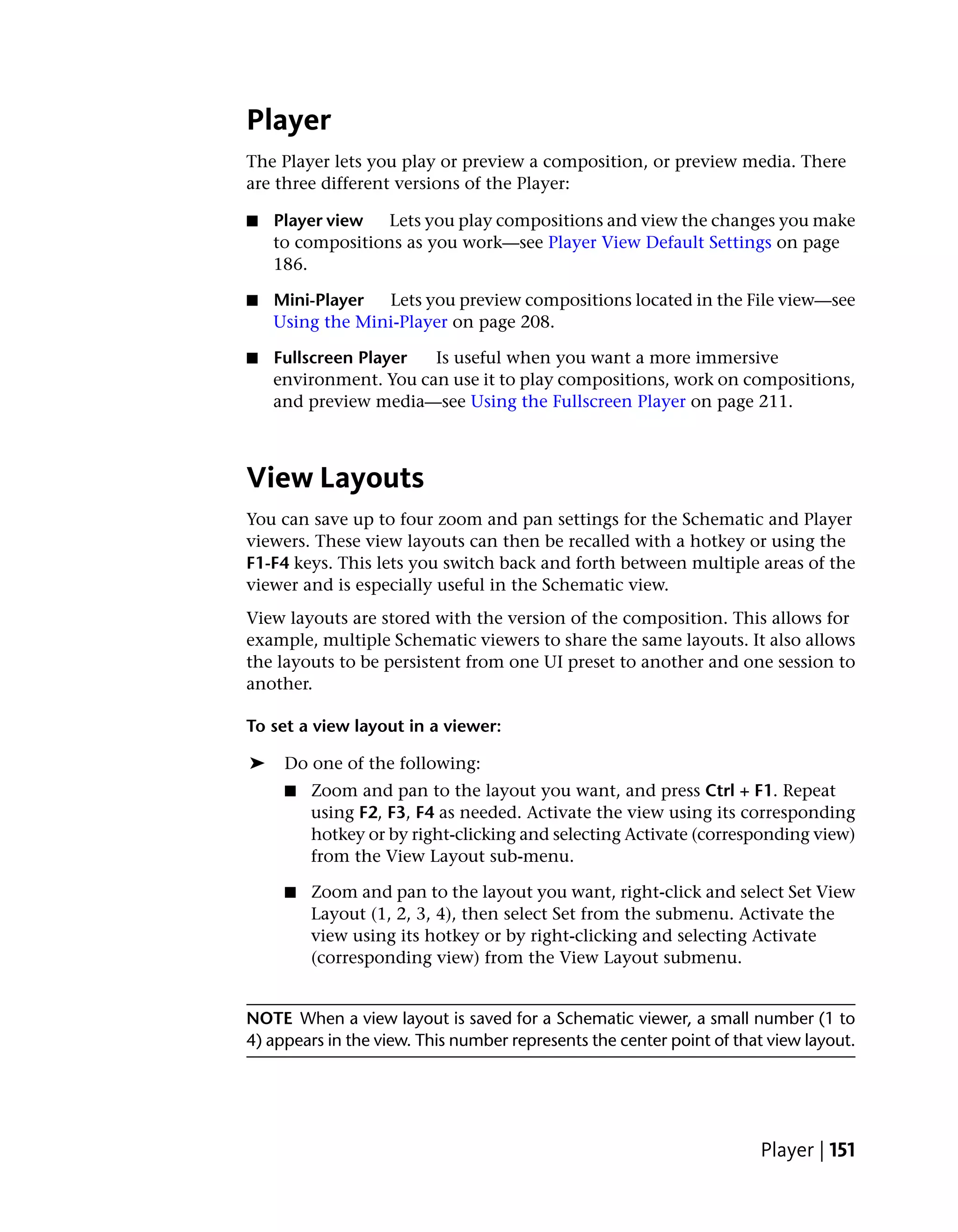
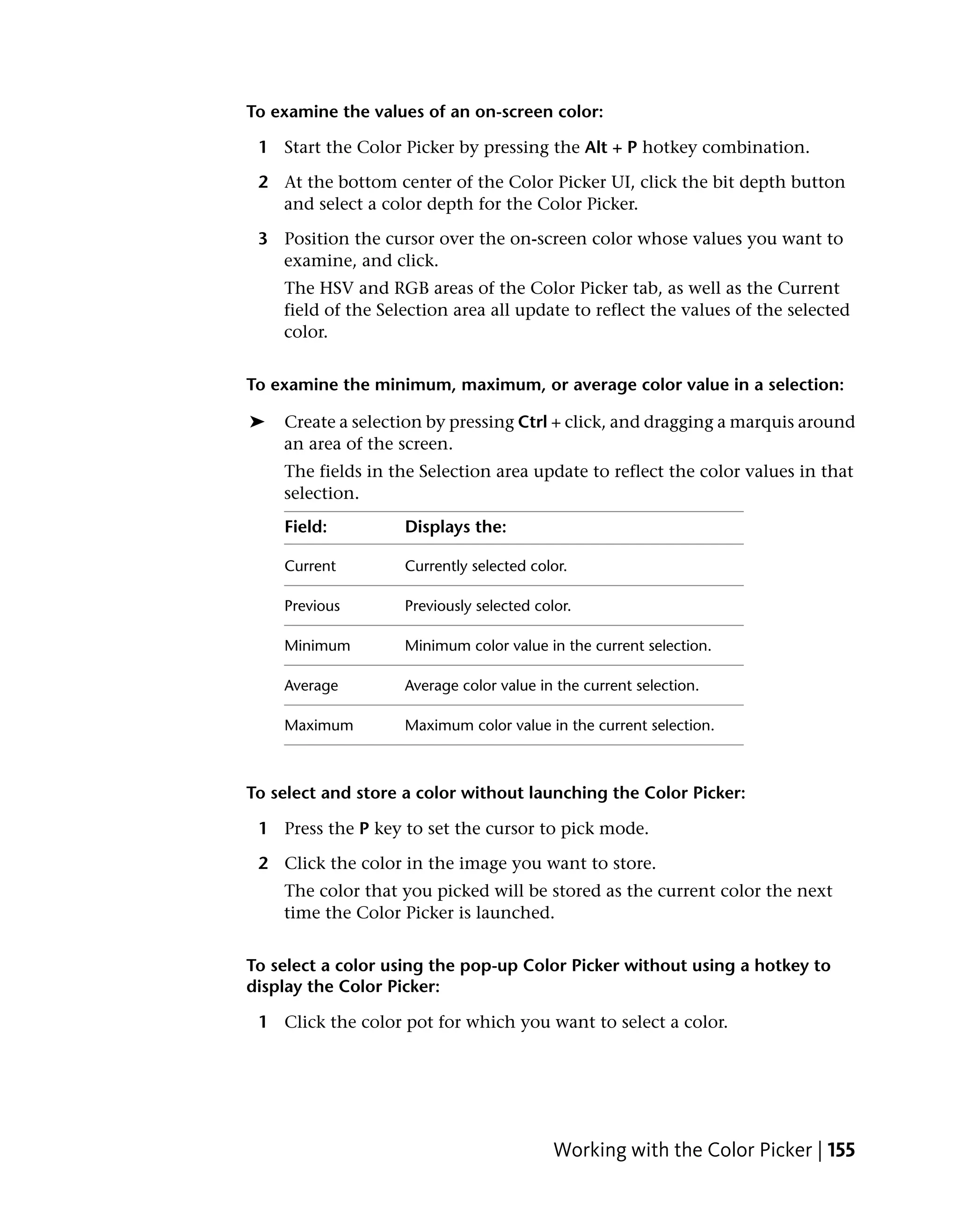
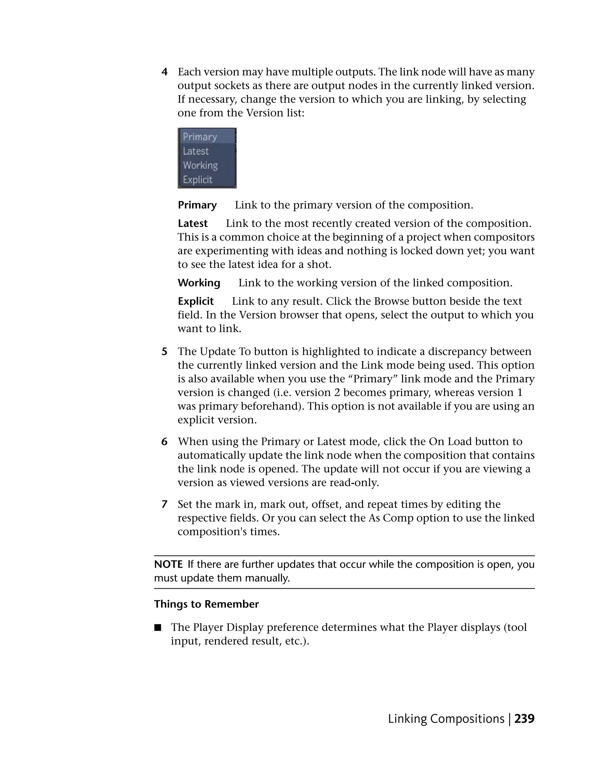
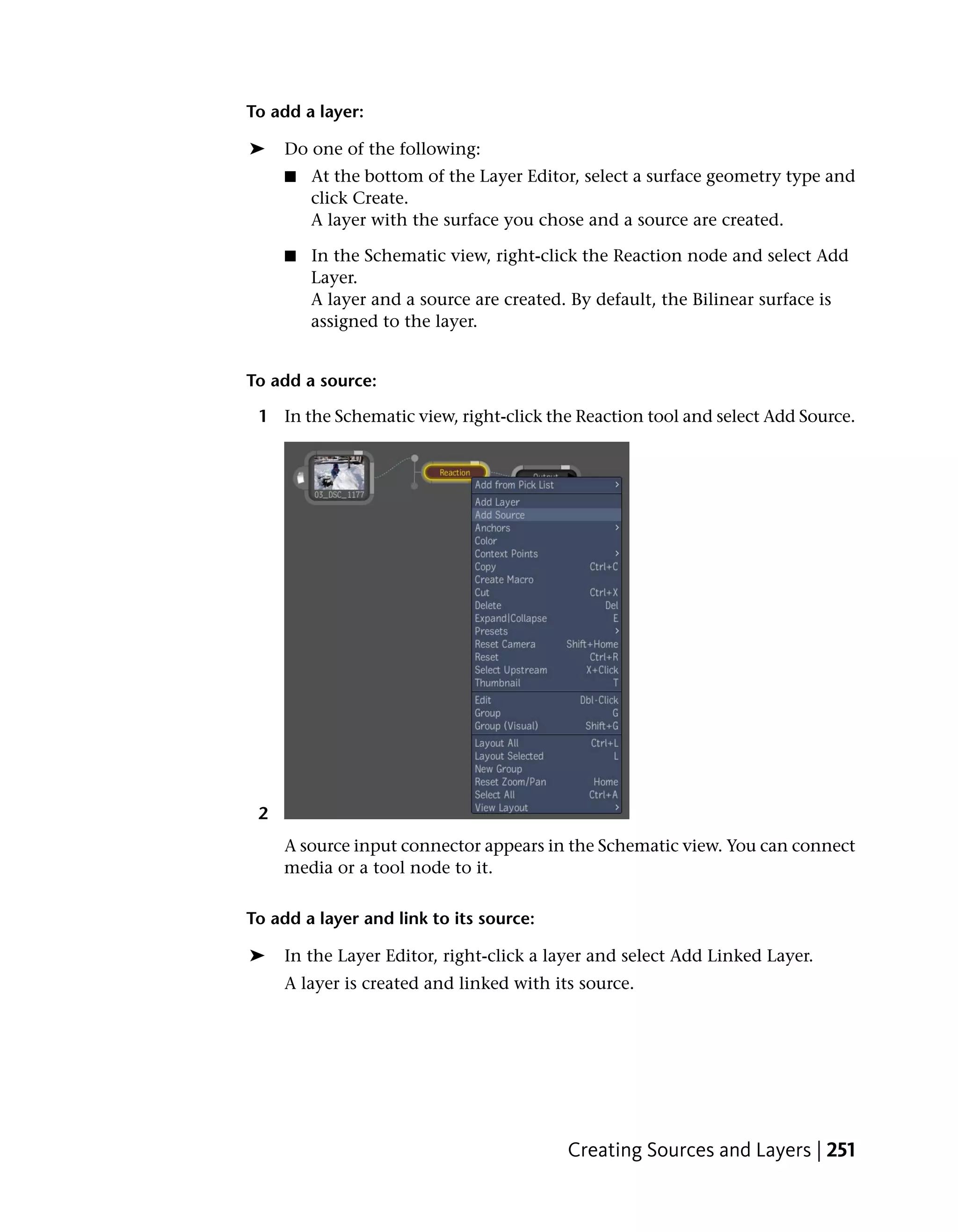
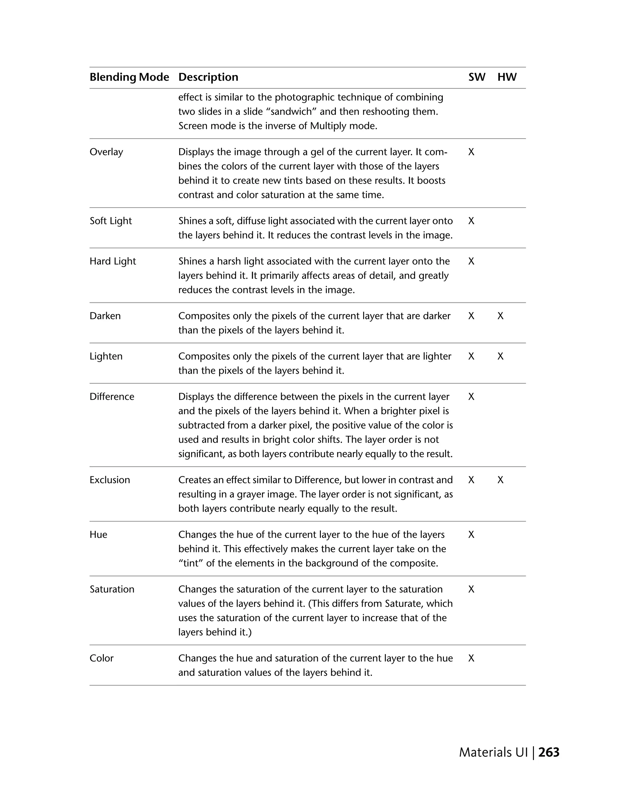
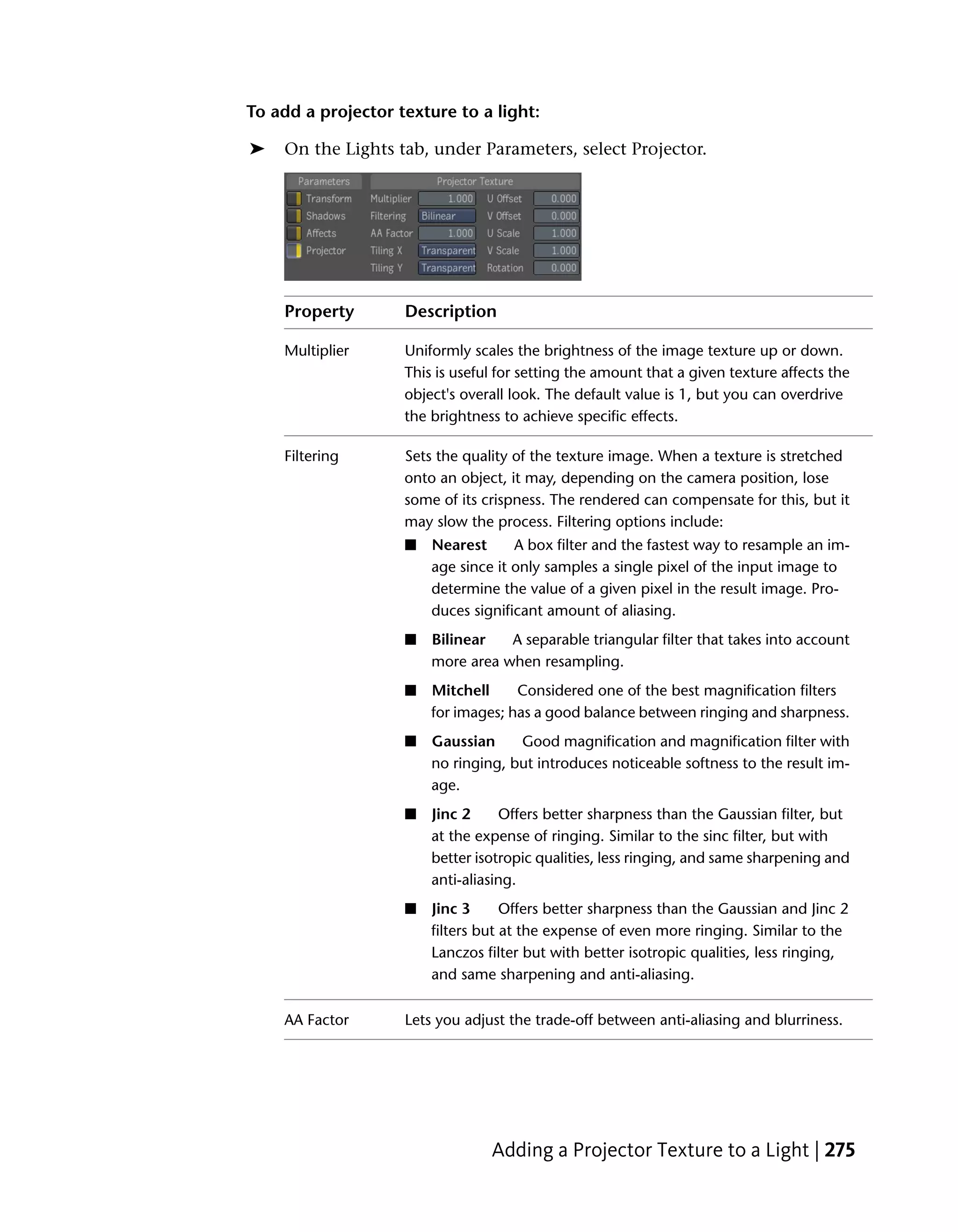
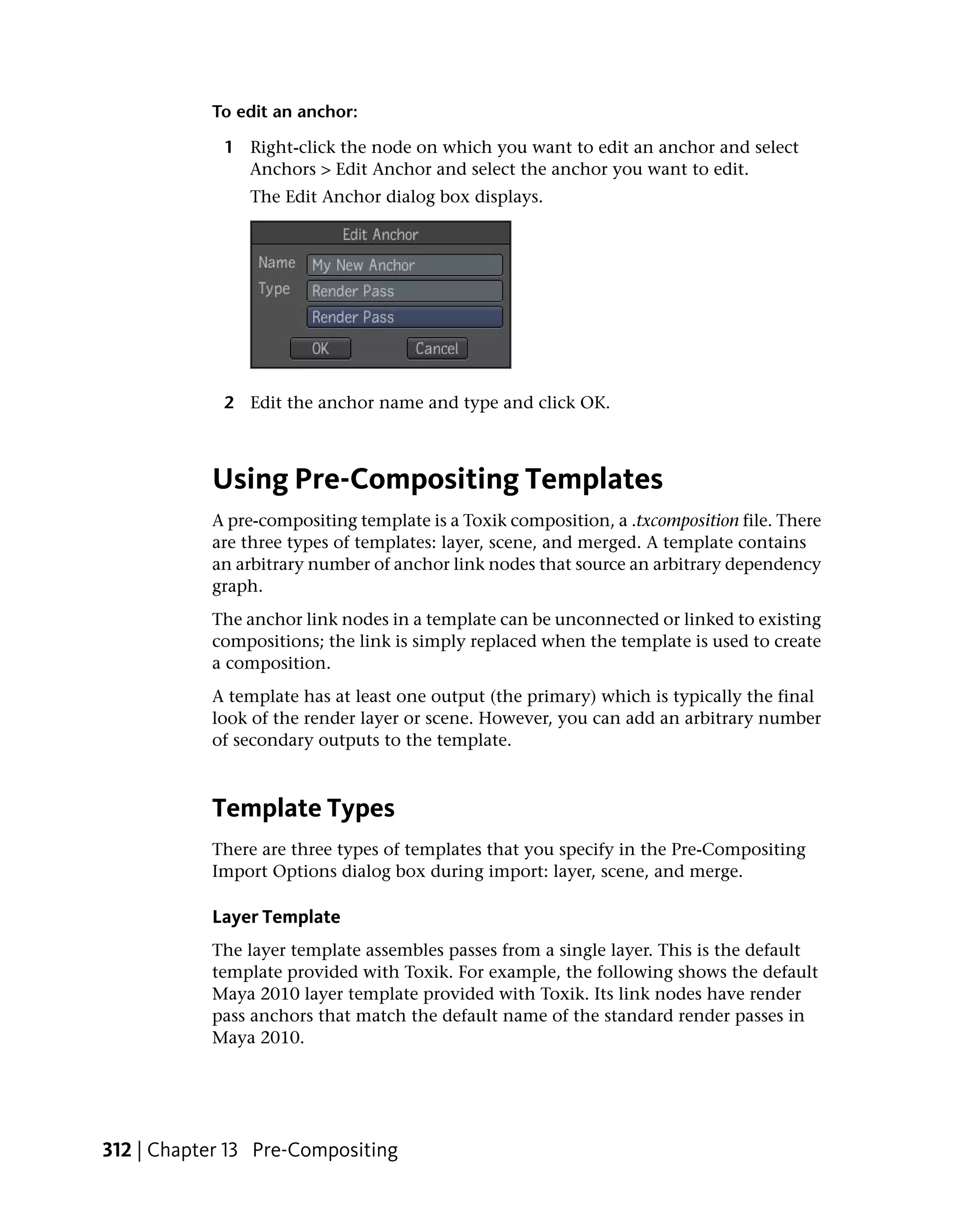
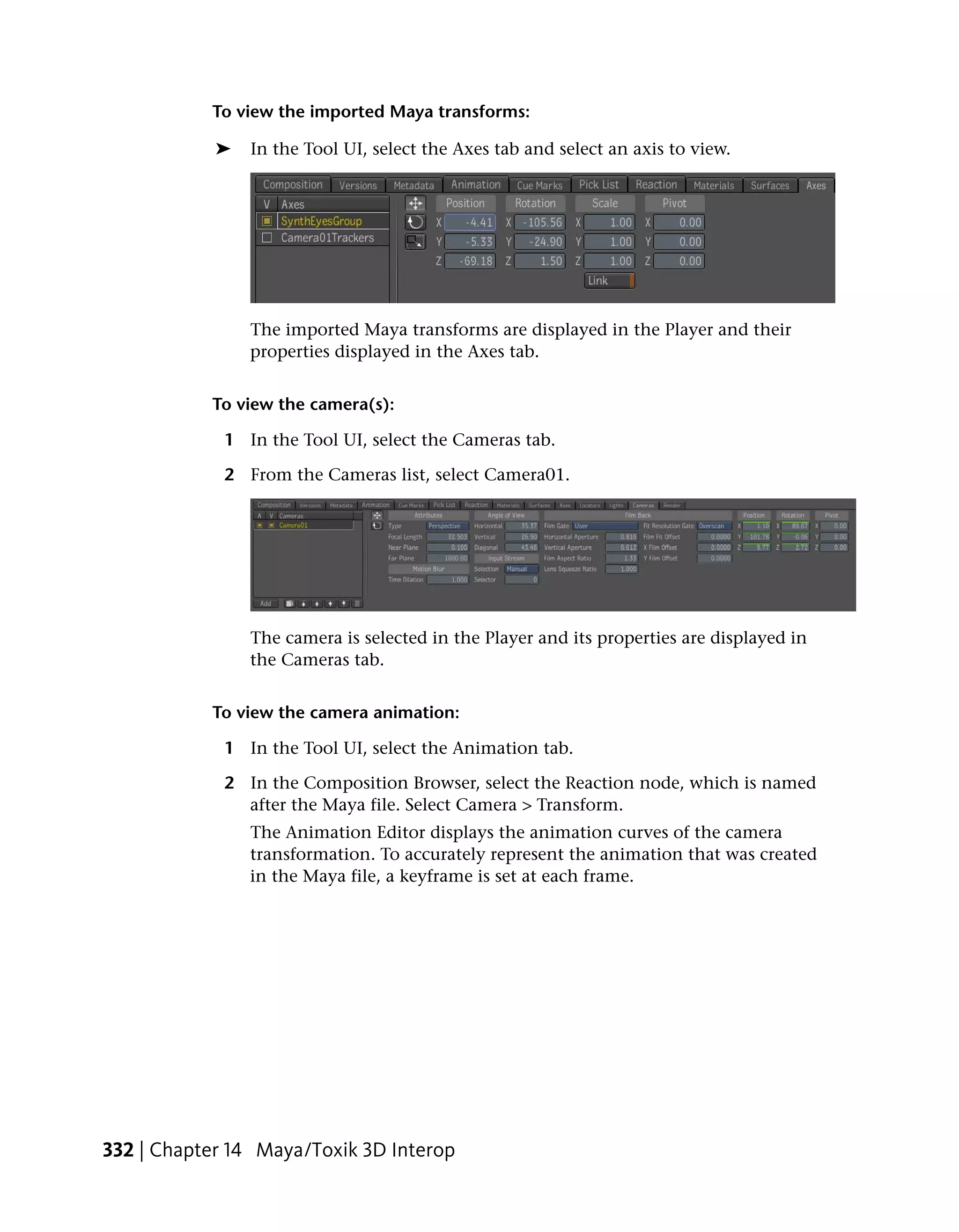
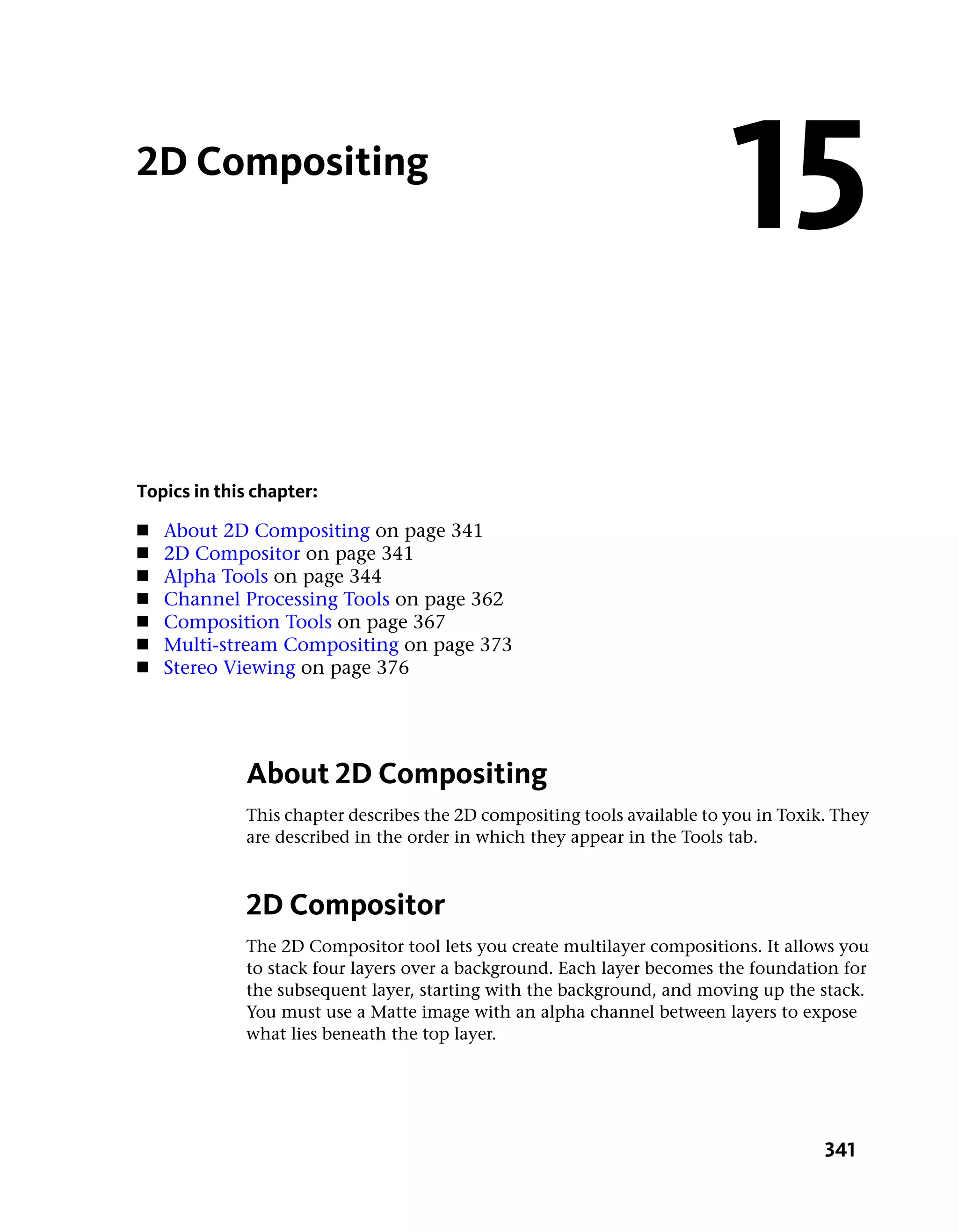
The Comp Alpha tool has the following parameters:
■ Front Channel Selects which channel to use for the front (default is
alpha).
■ Front Invert Inverts the front before o using it (default is off).
■ Front Intensity Specifies the intensity of the front layer. Default is 100%
and range is [0,1].
■ Front Opacity Controls the opacity of the front in the compositing. If
the opacity is less then one, the front will get more transparent and you
will start seeing the back through it. Default is 100%; range is [0,1].
■ Back Channel Selects which channel to use for the back (default is alpha).
■ Back Invert Inverts the back before using it (default is off).
■ Back Intensity Specifies the intensity of the back layer. Default is 100%;
range is [0,1].
■ Comp Mode Determines which compositing mode will be used (default
is Over)—see Compositing Operators on page 354.
■ Correlation Specifies how the two input mattes are correlated. This can
be used to improve the quality of the composite in special cases. For
example, if you composite two mattes that share a good portion of their
outline, you should indicate if they are Adjacent or Superposed. By default,
the correlation mode is None, assuming that normally, the input mattes
are not correlated.
Comp Alpha Tool | 353](https://image.slidesharecdn.com/mayacompositeuserguide-1260452105-phpapp01/75/Mayacompositeuserguide-369-2048.jpg)

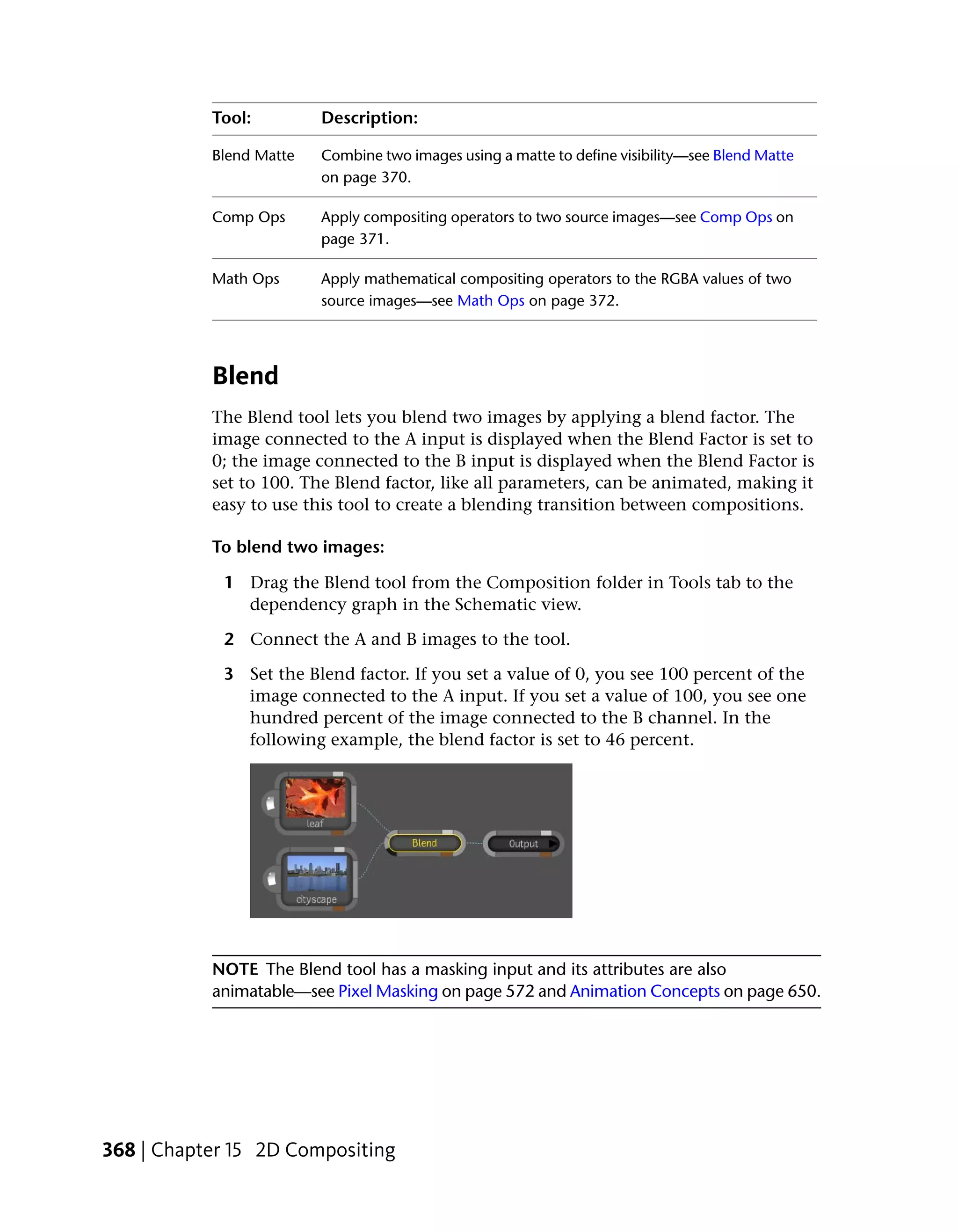
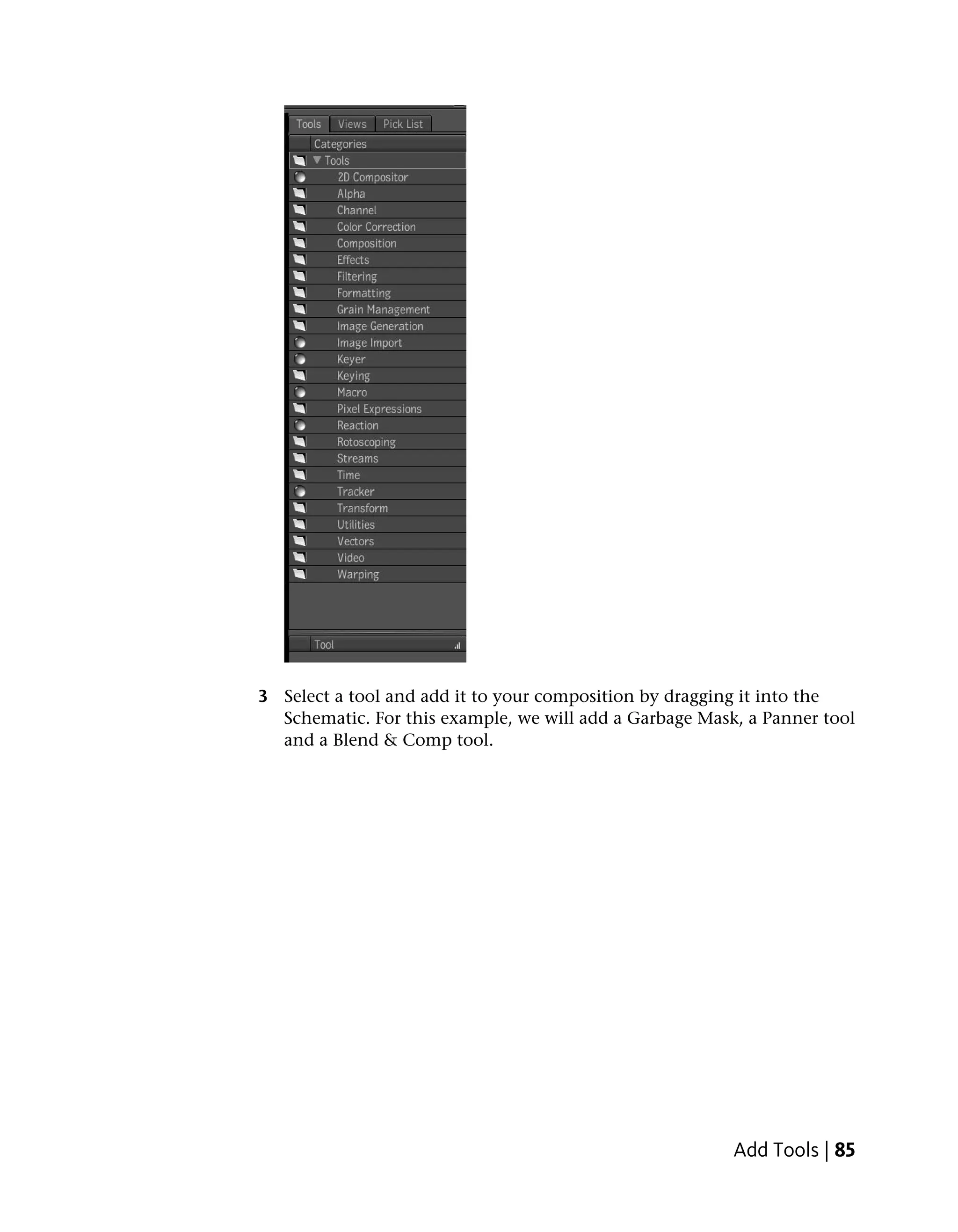
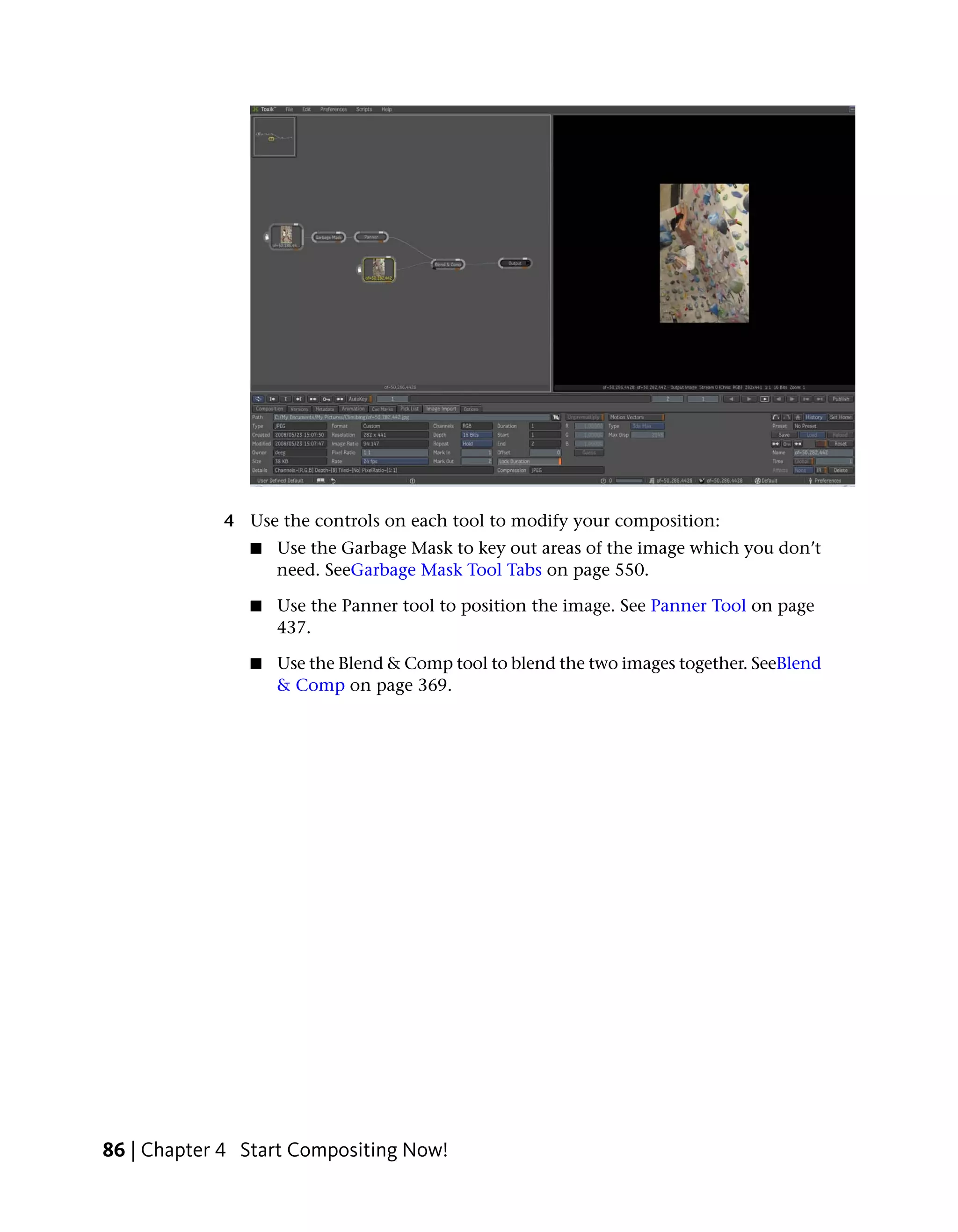
![Blend & Comp
The Blend & Comp tool is used to composite front and back RGBA images.
While most compositing tools composite a front layer over an opaque
background under the direction of a matte image, this tool offers full support
for RGBA images, both for the front and back inputs, and computes an RGBA
result.
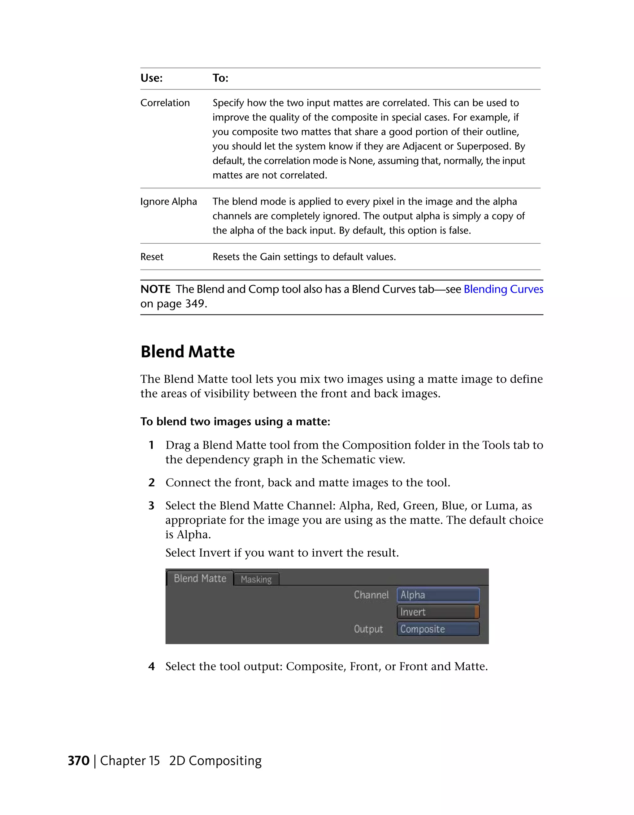
You can specify a compositing operator to control the shape of your output
and a blend mode to determine how the front and back are combined in the
areas where they overlap.
The Blend & Comp tool is in the Composition folder in the Tools tab, and
has the following parameters:
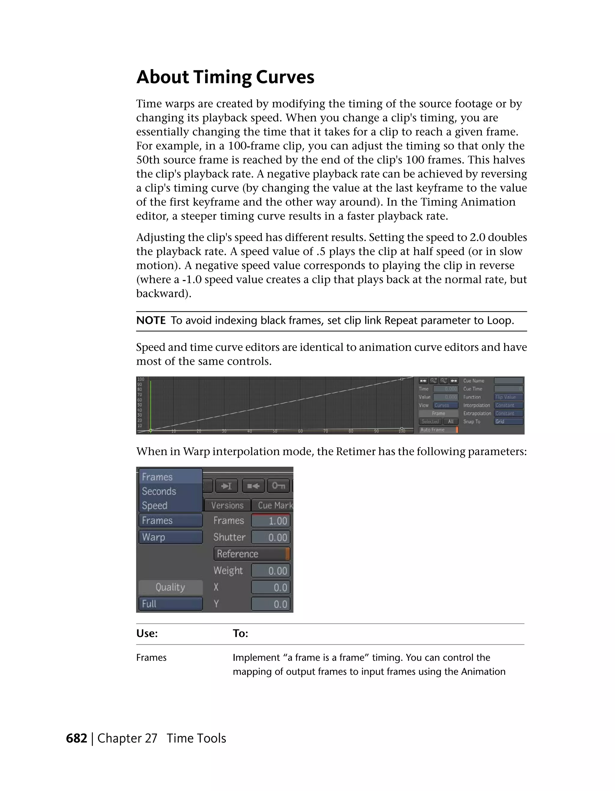
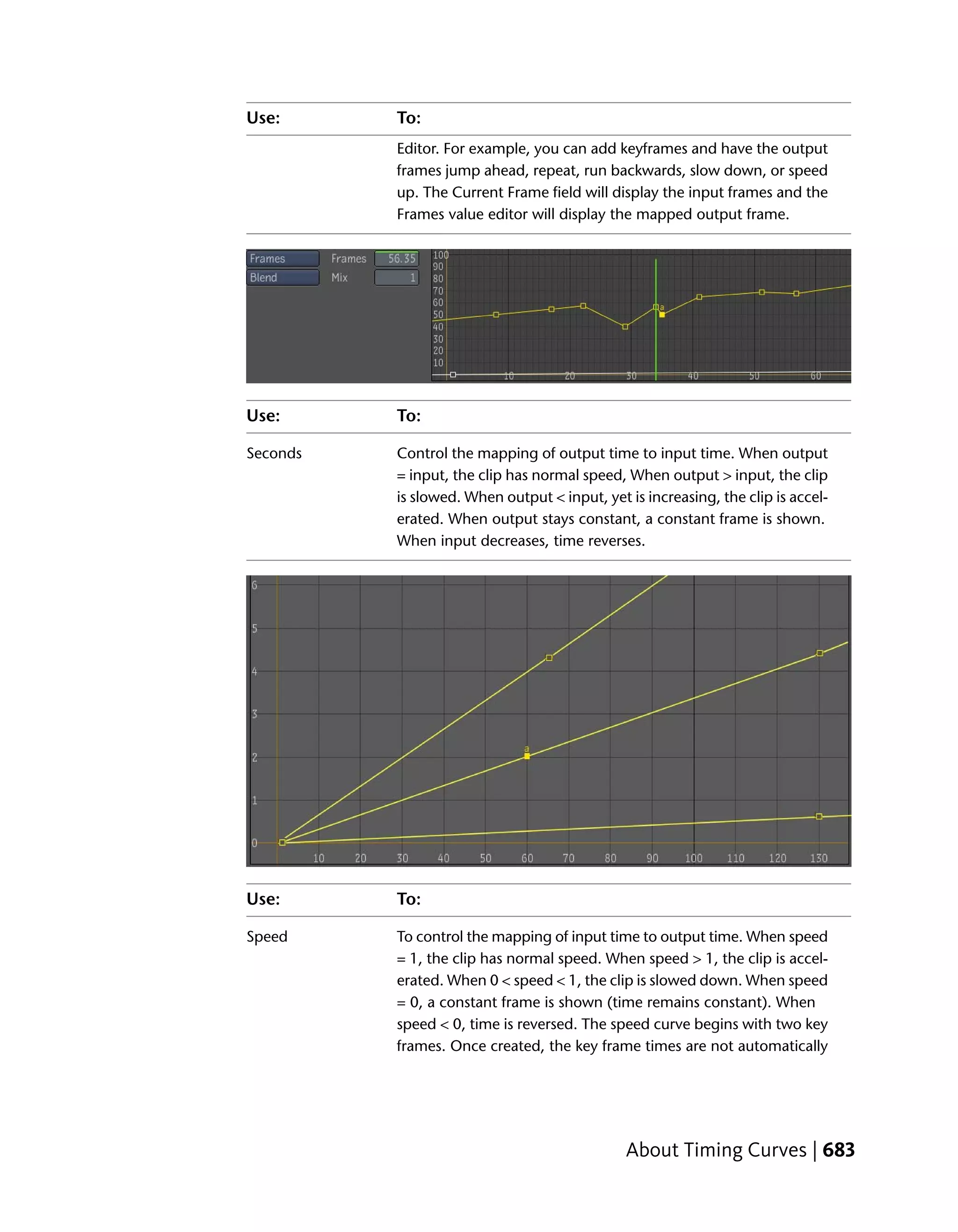
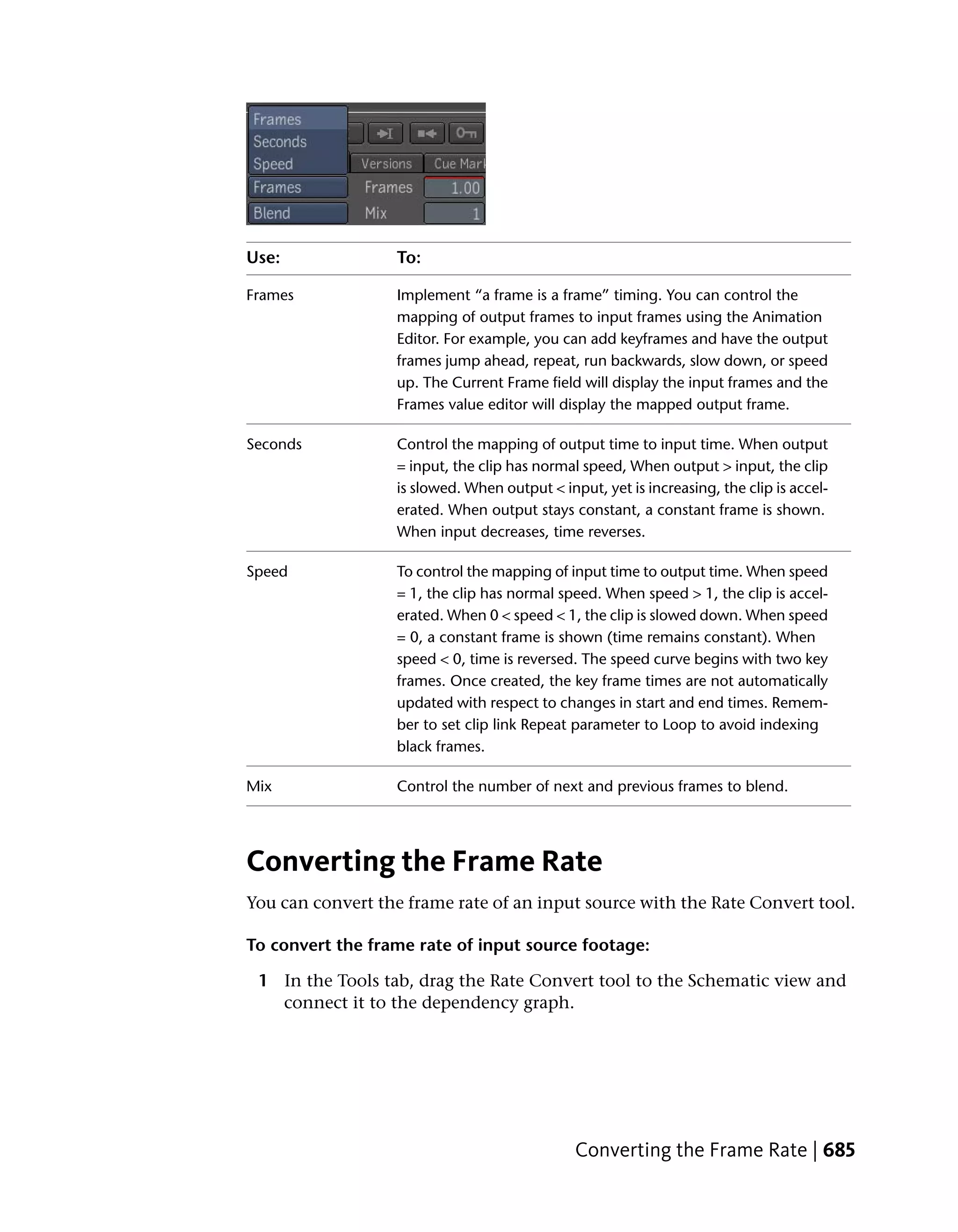
Use: To:
Front Gain Multiply the front by a color factor prior to using it in the blend. The
default is 100%; the range is [0,10].
Front Opa- Control the opacity of the front in the compositing. If the opacity is less
city than one, the front will be more transparent and you will start seeing
the back through it. The default is 100%; the range is [0,1].
Back Gain Multiply the back by a color factor prior to using it in the blend. The
default is 100%; the range is [0,10].
Back Opacity Control the opacity of the back in the compositing. If the opacity is less
then one, the front will be more transparent and you will start seeing
the back through it. The default is 100%; the range is [0,1].
Comp Determine which compositing mode will be used (the default is
Over)—see Compositing Operators on page 354.
Blend Determine which blend mode will be used (the default is Normal). Click
the Blend button to view other available modes—see Blend Modes on
page 347.
Blend & Comp | 369](https://image.slidesharecdn.com/mayacompositeuserguide-1260452105-phpapp01/75/Mayacompositeuserguide-385-2048.jpg)


![LUT: 3 256
Each line following the header contains a single entry indicating the value to
which the source is converted. For example, a table converting 10-bit
logarithmic values to 8-bit linear would contain 1024 entries, corresponding
to the 0–1023 intensity range of pixels in the source file. Each of these entries
would be in the range 0–255, corresponding to the intensity range in the
destination.
Blank lines and comment lines (starting with a number sign [#]) are ignored.
Comment lines are useful for indicating the end of one table and the beginning
of another, or for describing how the script or program works.
Floating Point 1D LUT File Format
Floating point LUTs are supported and are reversely compatible in most cases.
You can specify your own floating-point 1D LUT using an ASCII editor as long
as it is in the correct format and is named correctly.
The following illustration represents a 1D floating-point LUT that consists of
one channel of five values that fall between the range of 0.0 and 2.0.
610 | Chapter 25 Color Correction](https://image.slidesharecdn.com/mayacompositeuserguide-1260452105-phpapp01/75/Mayacompositeuserguide-626-2048.jpg)
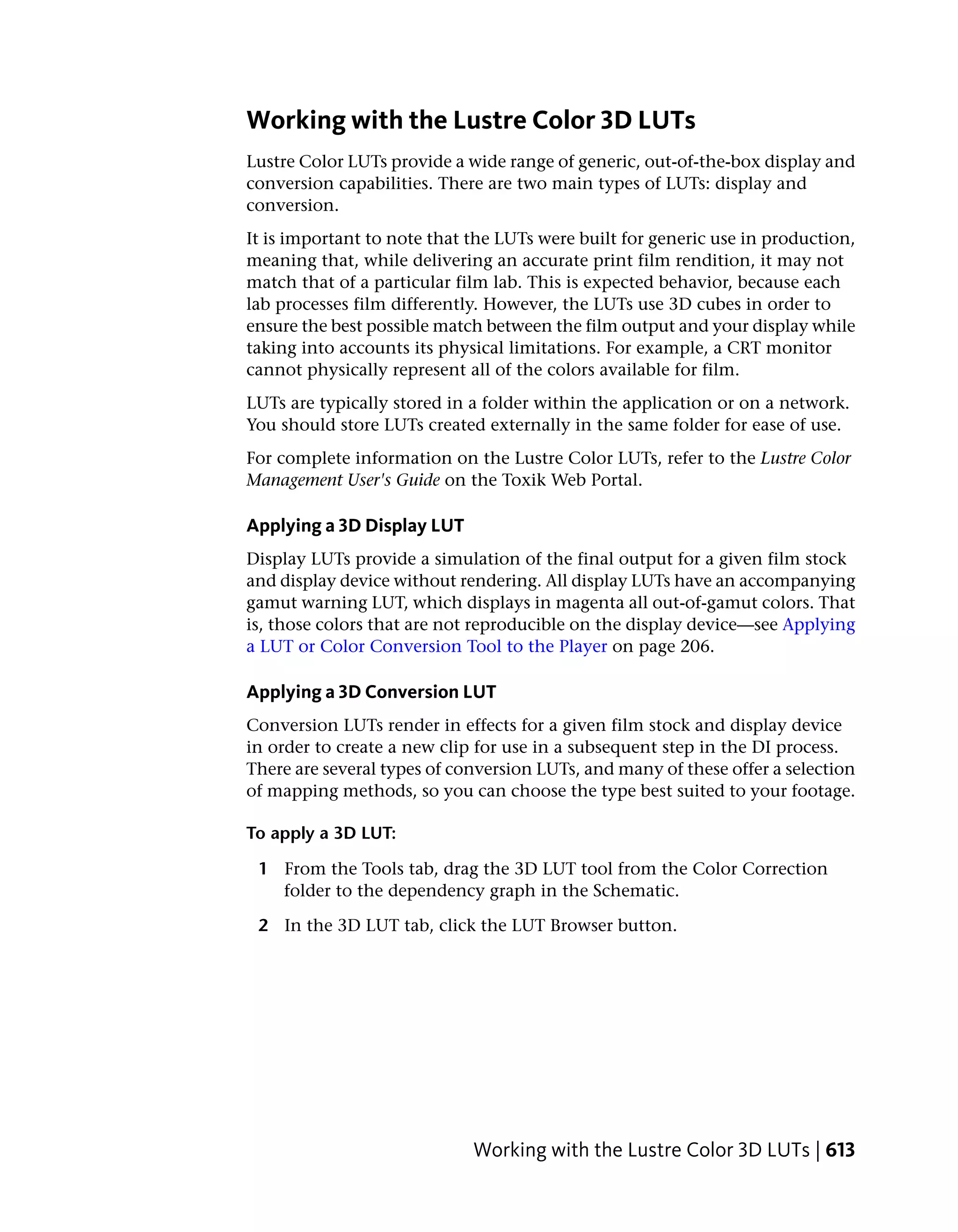
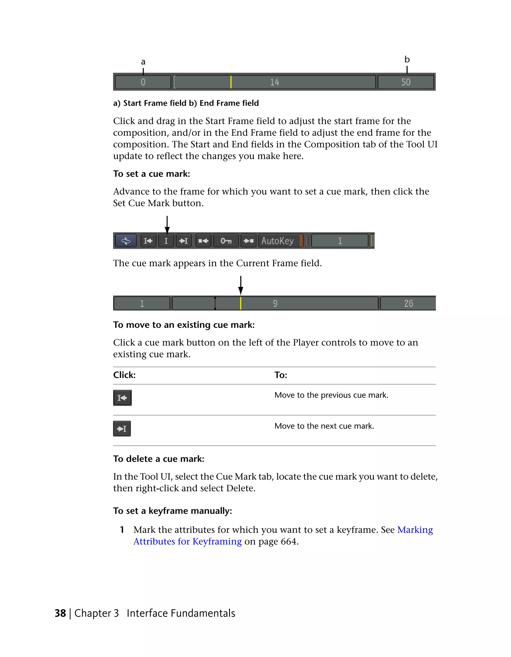
![(a) Input (b) Output
NOTE The CC Histogram's input and output level controls' fields are animatable
attributes—see Setting Keys Manually on page 666 and Validating and Applying
the Expression String on page 705.
Input Sliders
The Input sliders below the histogram viewer are used to control the range of
input color values in the image. The white slider on the right sets the
maximum value for the range. The black slider on the left sets the minimum
value for the range.
The histogram shown in the main tab is that of the selected channel creating
a total of four possible histograms. The histogram background color matches
that of the selected channel: gray for luminance, red, green, or blue.
All main tab values are shown in the range [0 to 1].
The input slider controls the values that are clamped to 0 (below the minimum)
and to 1 (above the maximum). Values in between are scaled from 0 to 1. You
can also use this to increase contrast.
You can set the maximum and minimum limits for the color range by entering
the values in the Input fields on either side of the histogram.
NOTE Input levels increase contrast (remap more grays to blacks and whites),
while output levels decrease contrast (remap more blacks and whites to grays). If
you have an image that requires some softening of color or tone, the output levels
re-introduce some midtones to the image.
To increase contrast with the input sliders:
1 From the Tools tab, drag the CC Histogram tool from the Color Correction
folder to the dependency graph in the Schematic view.
CC Histogram Controls | 631](https://image.slidesharecdn.com/mayacompositeuserguide-1260452105-phpapp01/75/Mayacompositeuserguide-647-2048.jpg)
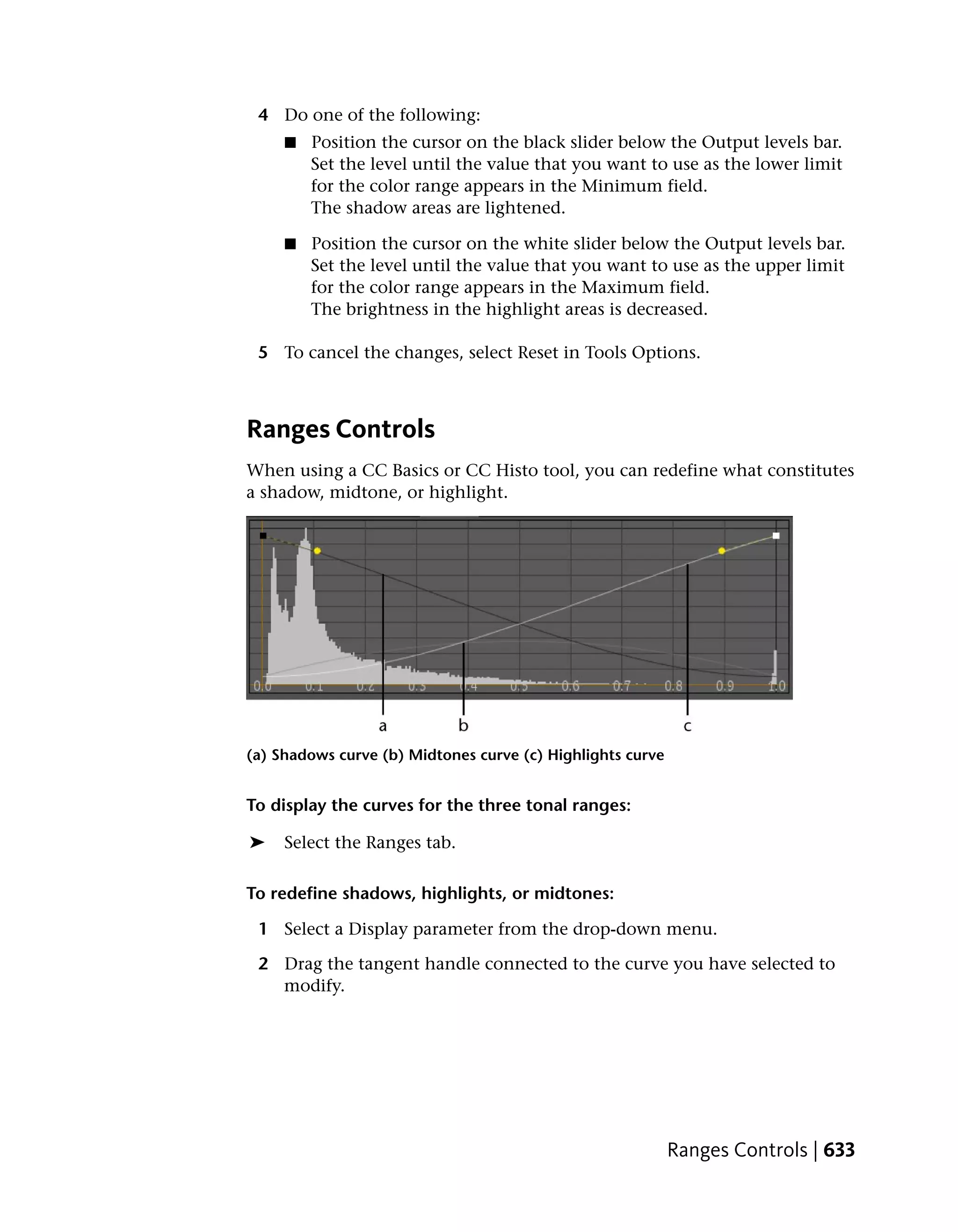
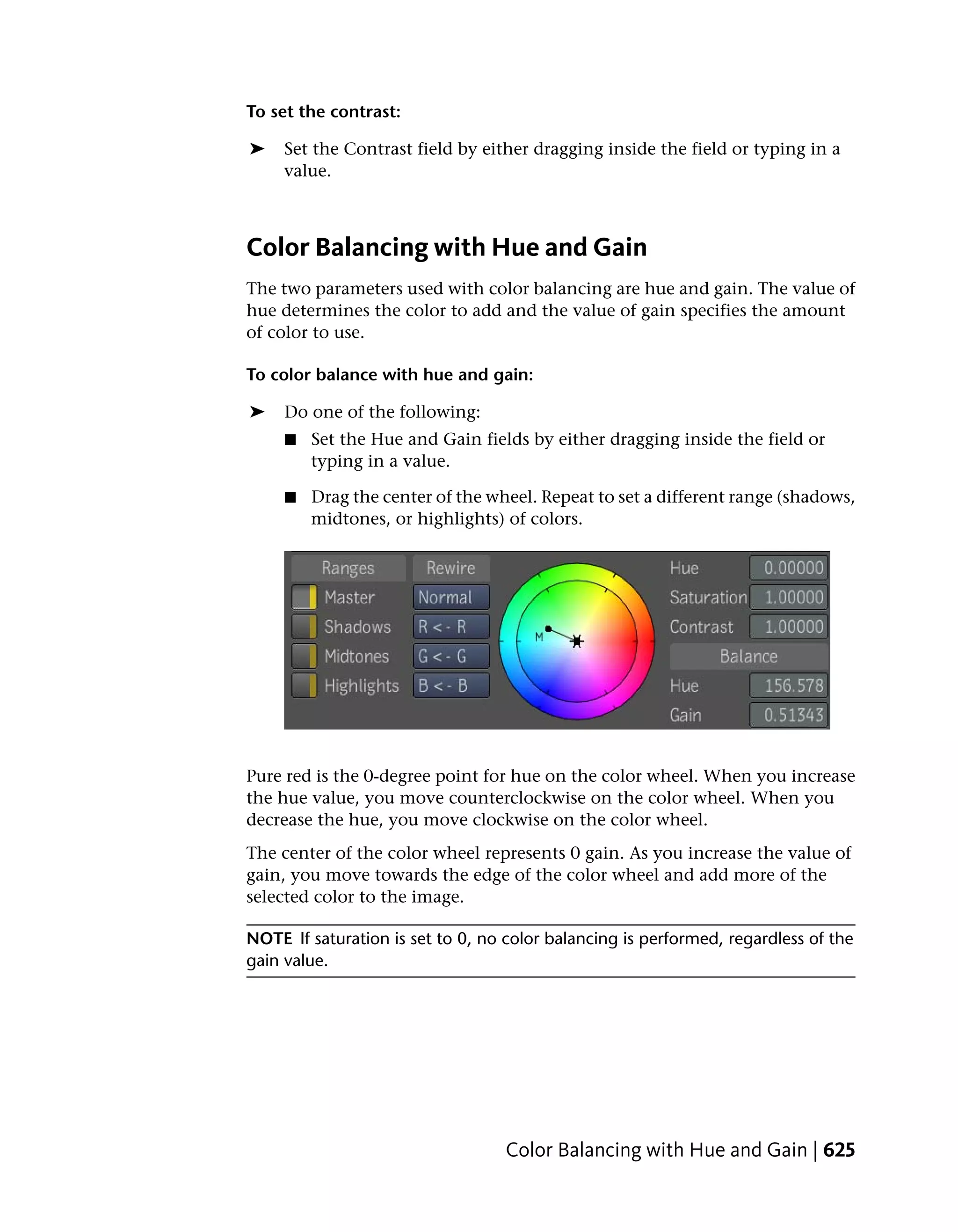
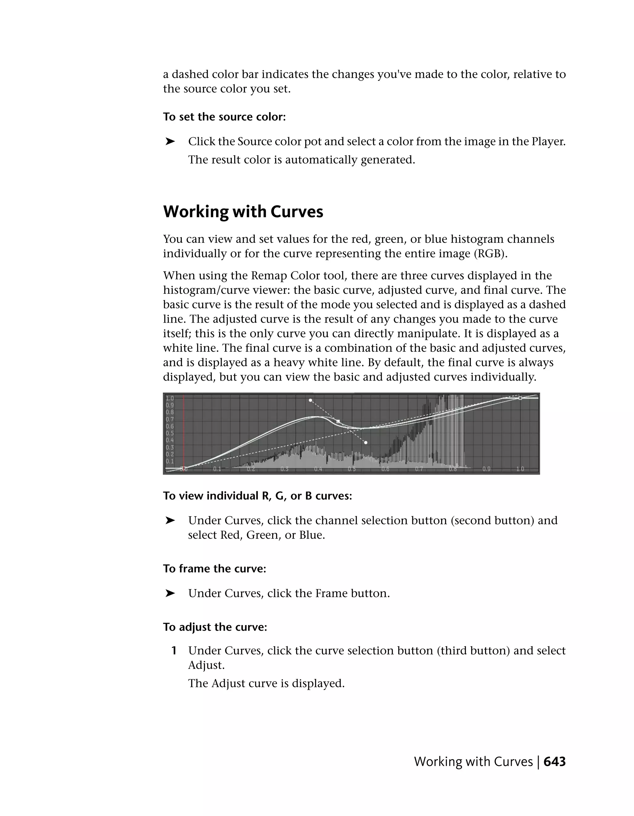
![To see the effects of the curves on color balance:
1 Open the CC Basics UI.
2 Under Balance, adjust the Hue and Gain to set the color balance for each
of the Shadow, Midtone, and Highlight ranges.
3 Go back to the Ranges controls and set the curves.
4 Go back to the CC Basics controls. Without changing the color balance
setup, note that the resulting image is different from that in step 1.
The difference is the result of the changes that were made to the curves
of the shadows, midtones, and highlights.
Clamp Color Tool
The Clamp Color tool lets you clamp colors that are outside a given color
gamut. This is useful when you want to clamp an HDR image before using it
with certain esoteric blend modes in a composite or when you want to clamp
negative color components before using other color correction tools. Most of
the time, you will want to clamp colors against the conventional [0,1] range,
so this is the default behavior of the tool. This tool is an image modifier; it
can be masked and muted and can only affect the RGB channels.
The Clamp color tool has the following parameters:
Use: To:
Min Set the minimum color values in the image to be clamped.
Max Set maximum color values in the image to be clamped.
As an aid in visualizing which pixels are affected by its operation, this tool
has two secondary outputs: It generates a one-channel image (a mask) where
all out of range pixels are set to one and the rest are set to zero. It generates a
pseudo-color image (a map) where all pixels that are below the range are
634 | Chapter 25 Color Correction](https://image.slidesharecdn.com/mayacompositeuserguide-1260452105-phpapp01/75/Mayacompositeuserguide-650-2048.jpg)


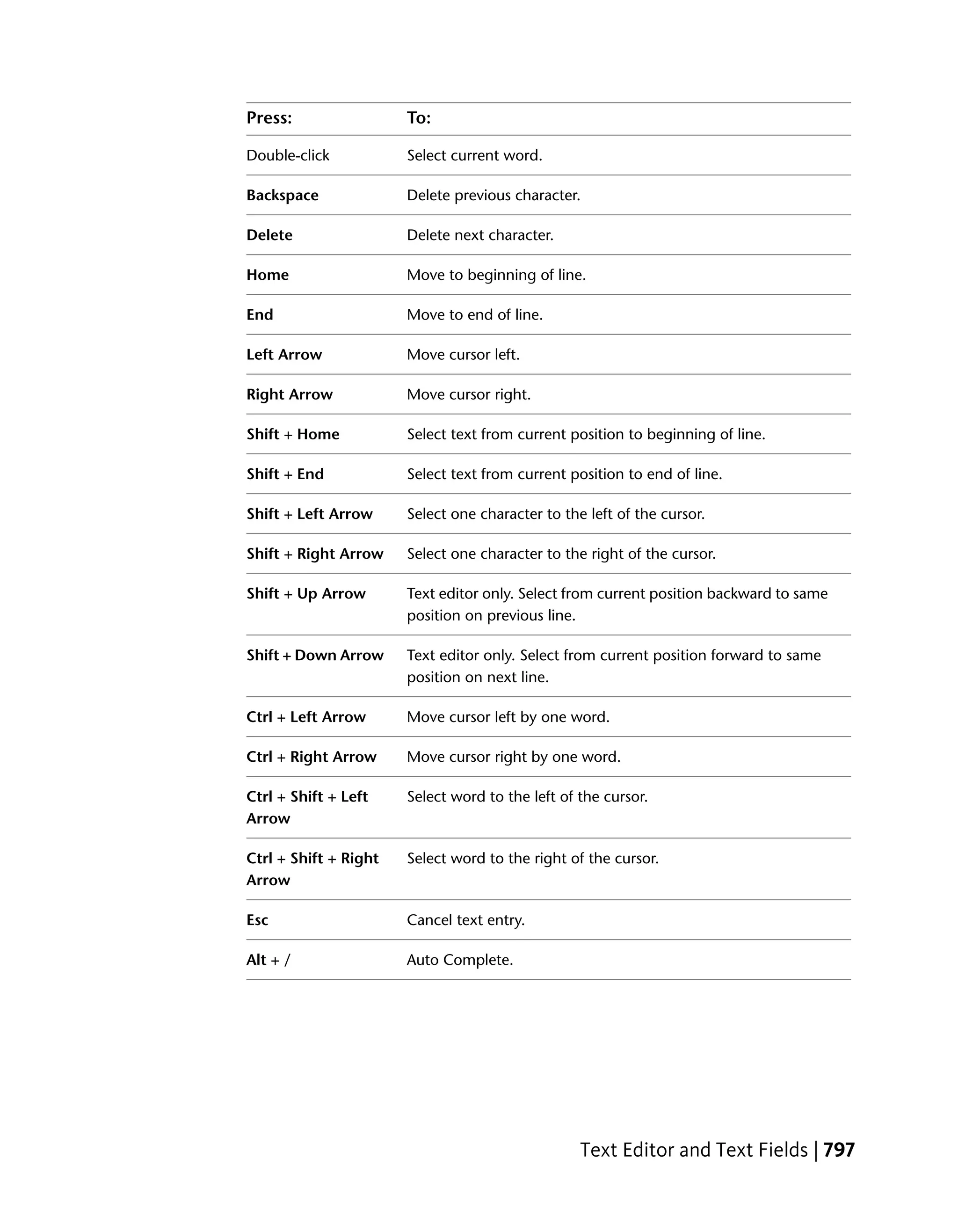
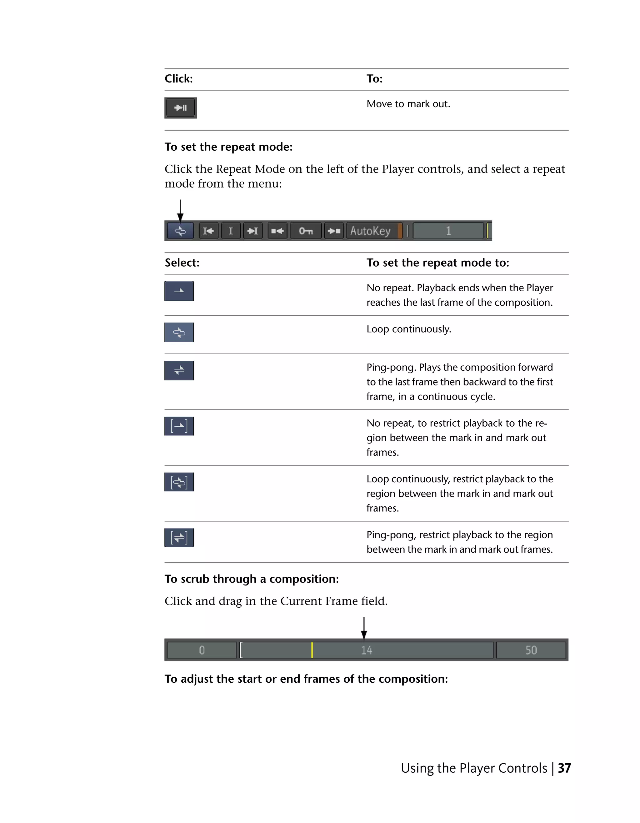
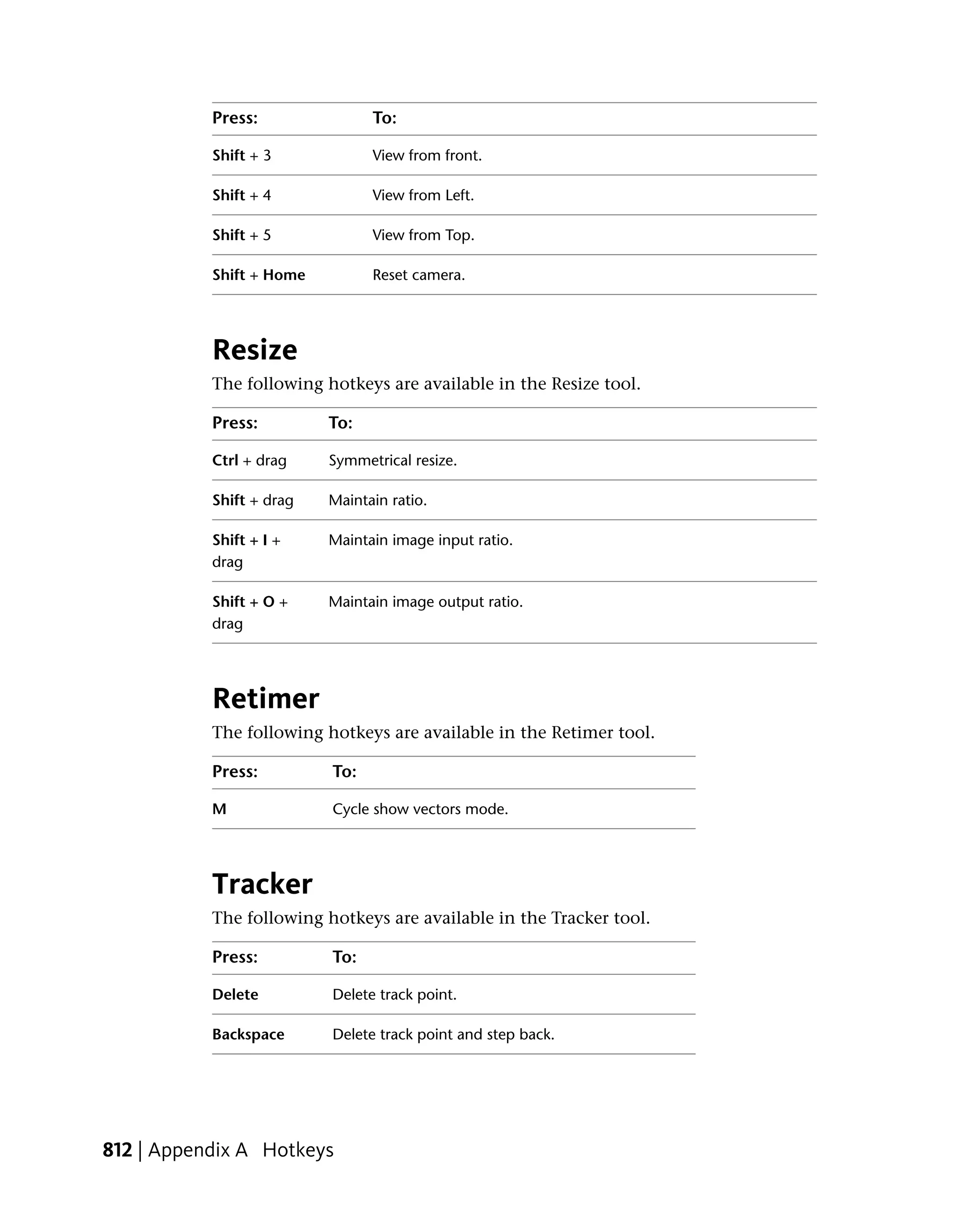
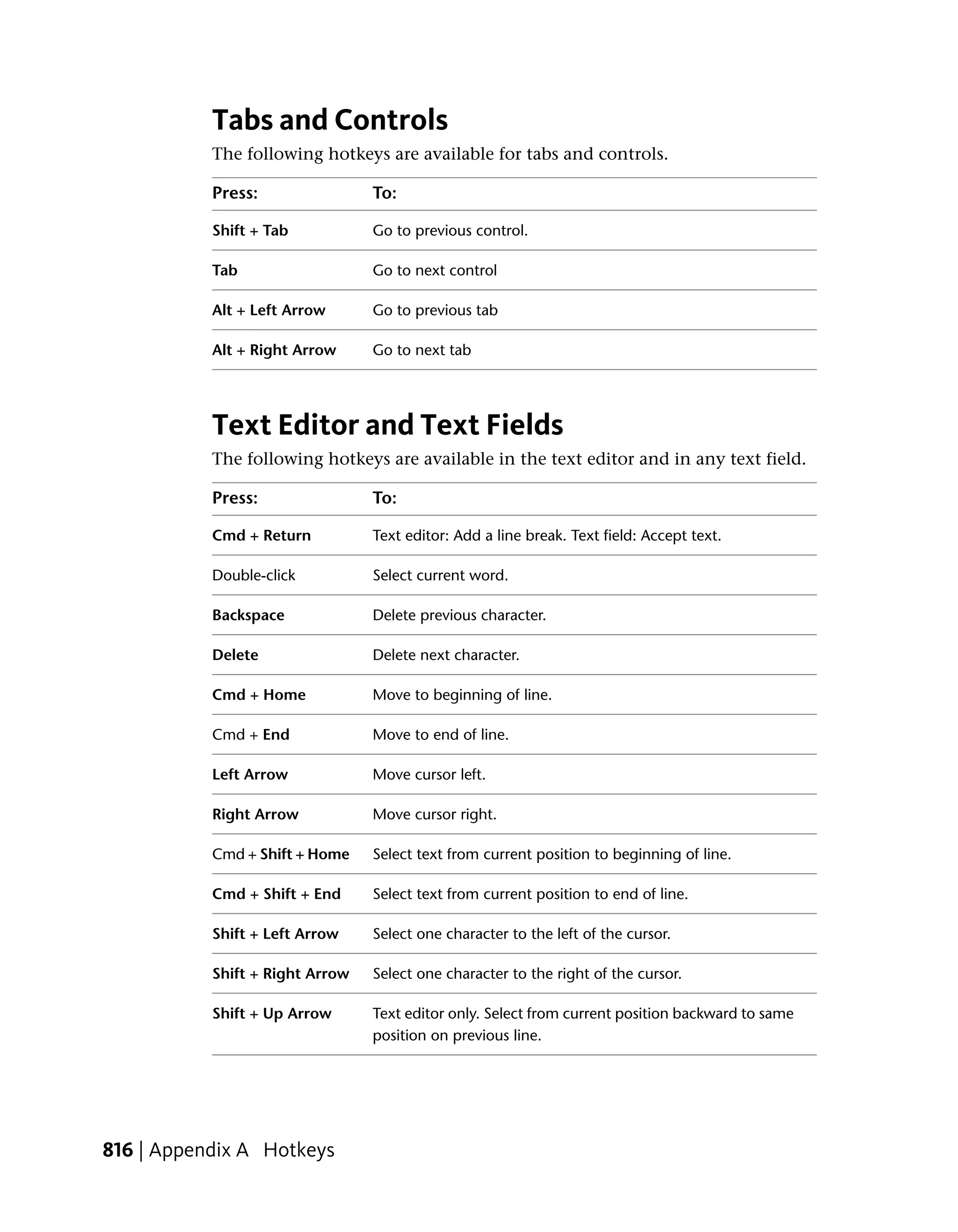
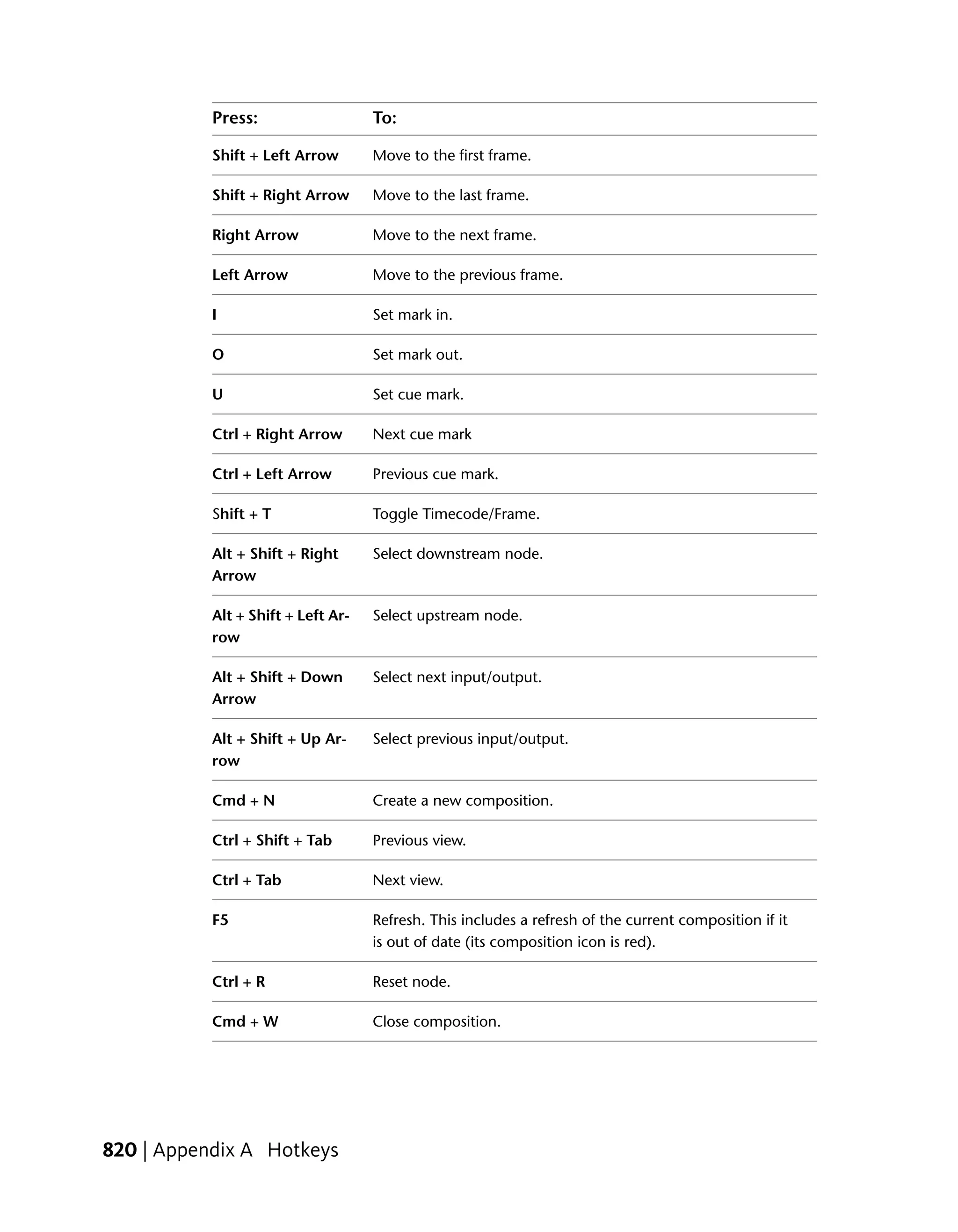
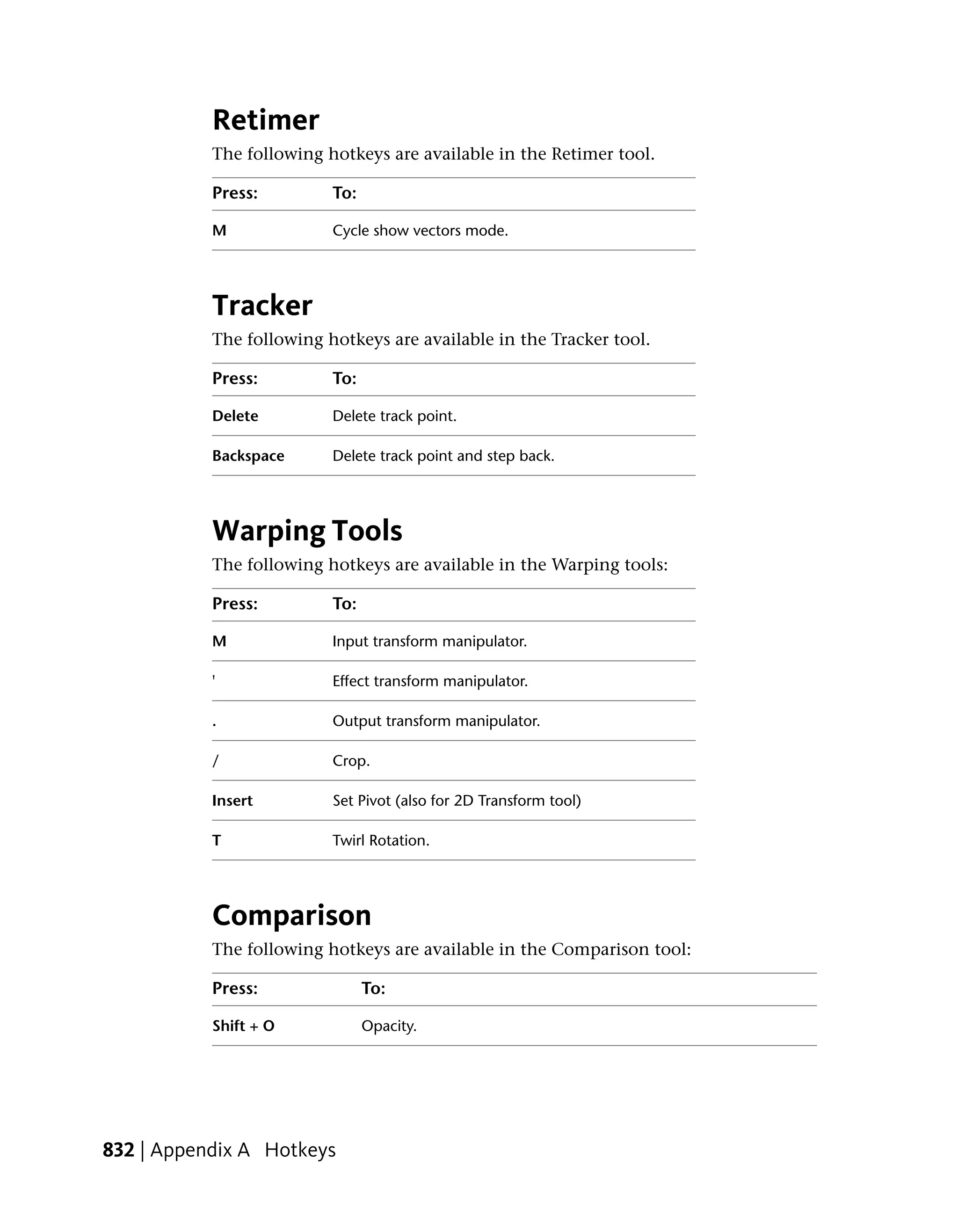
![Press: To:
Esc Cancel.
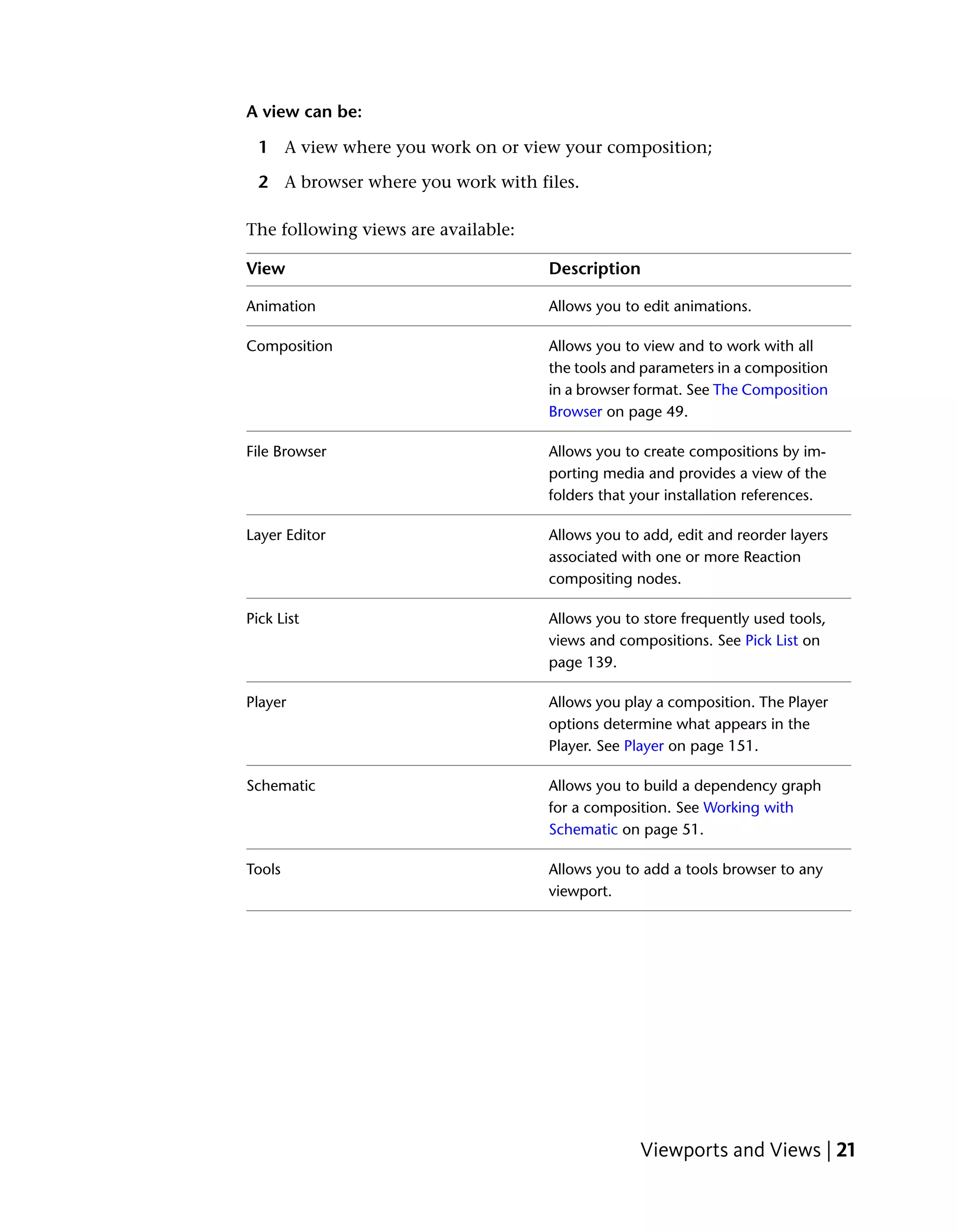
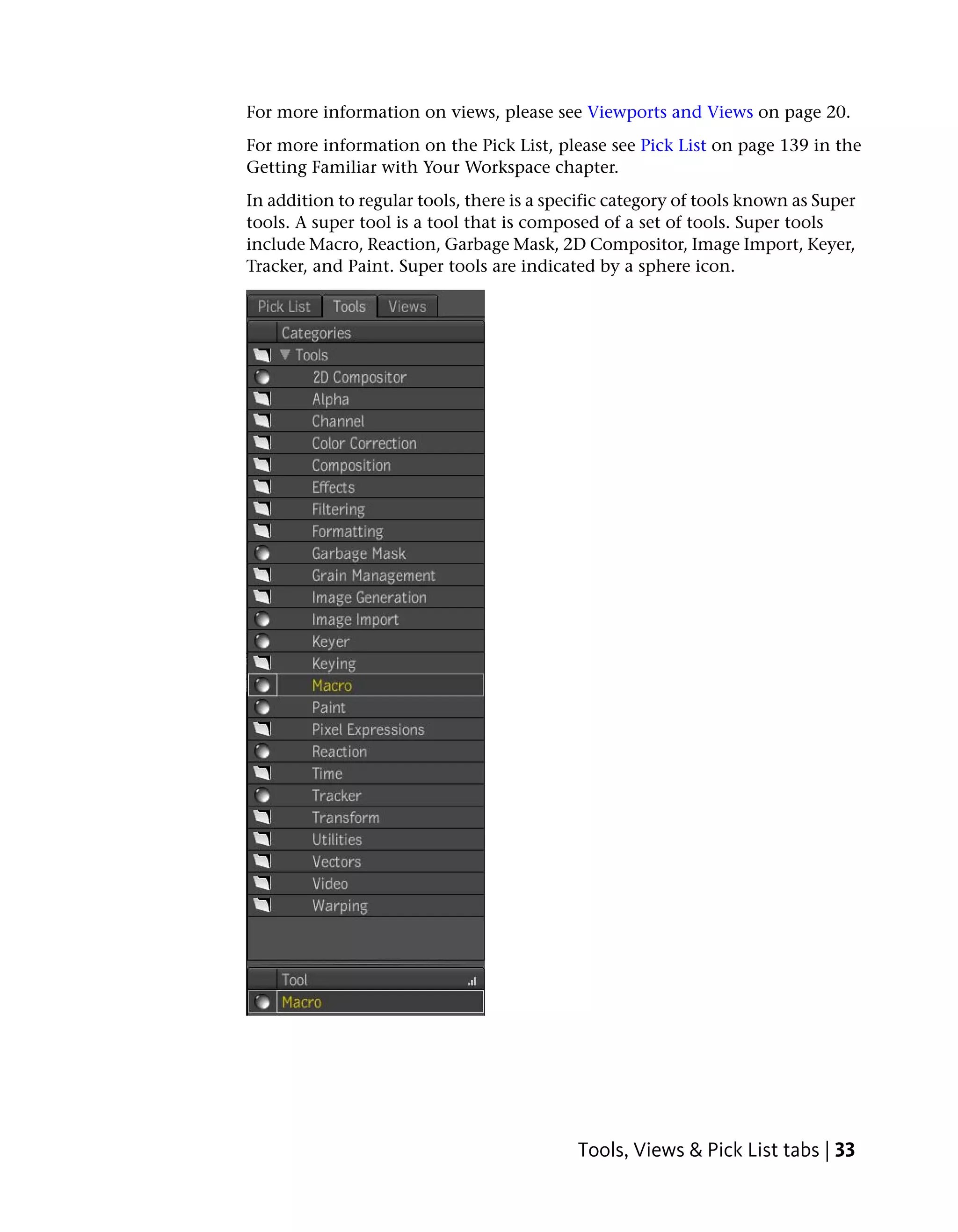
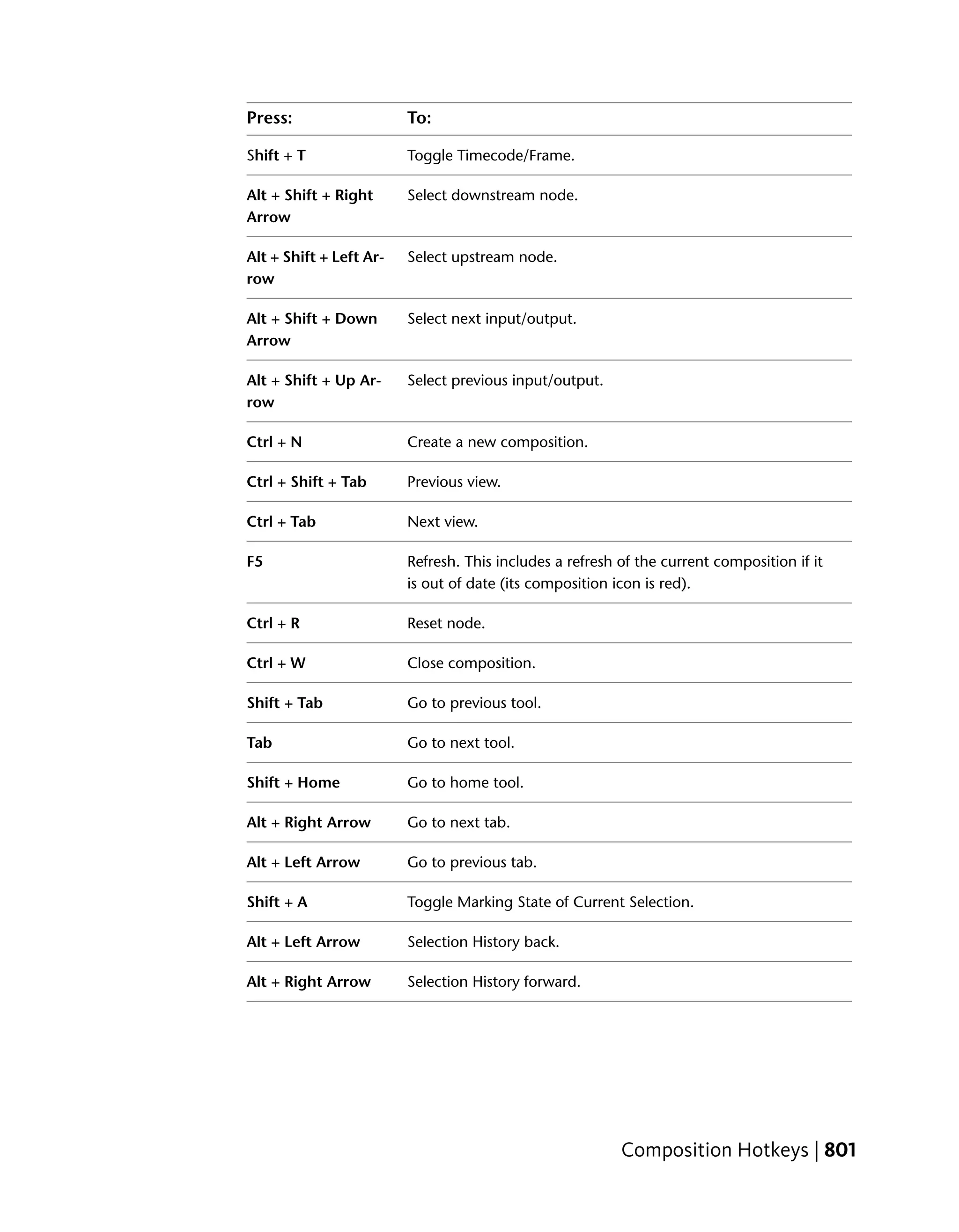
Views
The following hotkeys are available in Schematic, Animation Editor, and Player
views.
Press: To:
Spacebar + drag Pan
Home Reset zoom and pan.
Up Arrow Zoom in.
Down Arrow Zoom out.
Ctrl + Up Arrow Integer zoom in.
Ctrl + Down Arrow Integer zoom out.
Ctrl + Spacebar + Zoom
drag
Shift + Spacebar + Zoom region.
drag
Ctrl + Home Zoom selected items.
Ctrl + Alt + Home Zoom all scene.
[F1 - F4] Activate Viewpoint [1-4].
Ctrl + [F1 - F4] Set Viewpoint [1-4].
Ctrl + Shift + [F1 - Delete Viewpoint [1-4].
F4]
Views | 803](https://image.slidesharecdn.com/mayacompositeuserguide-1260452105-phpapp01/75/Mayacompositeuserguide-819-2048.jpg)
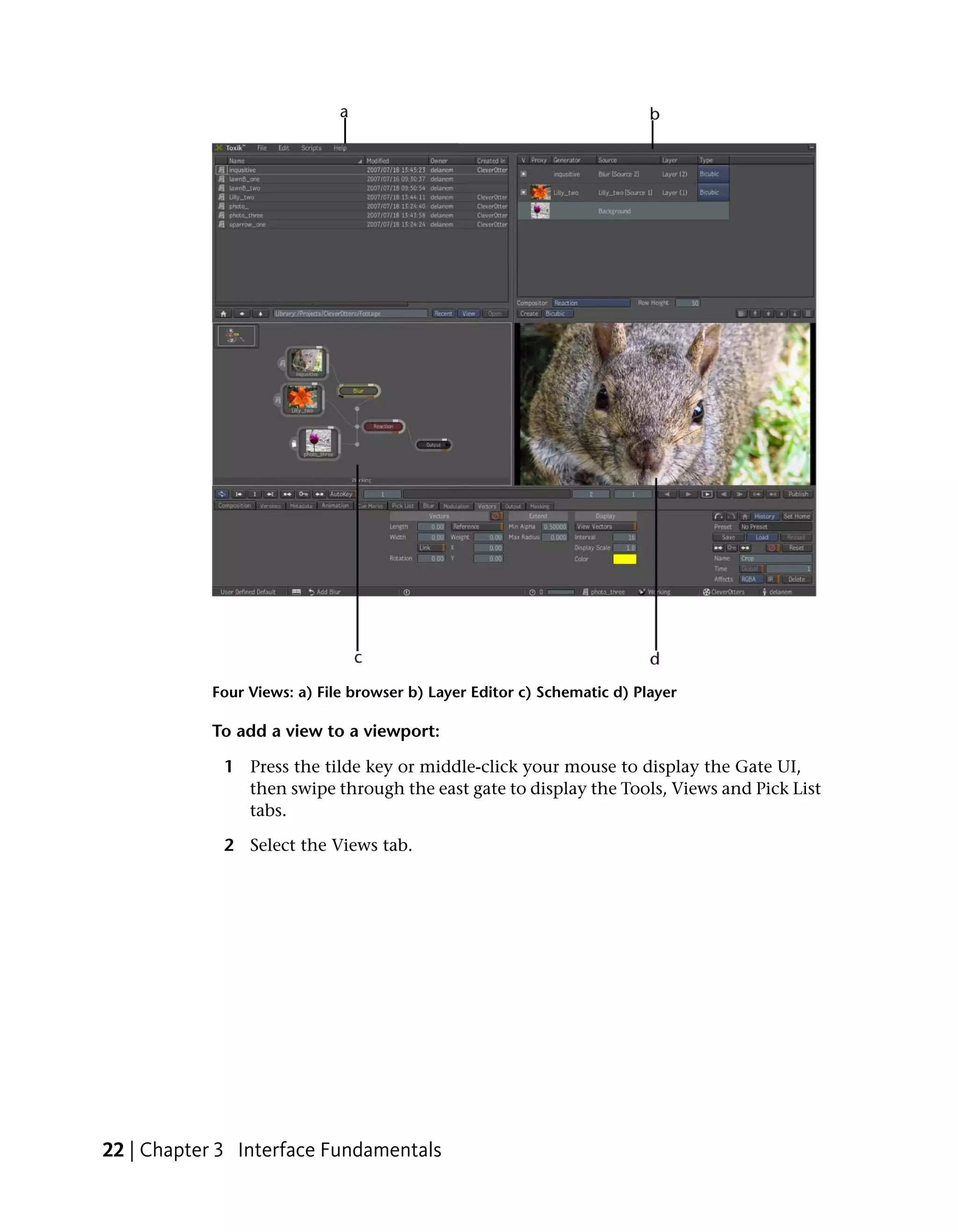
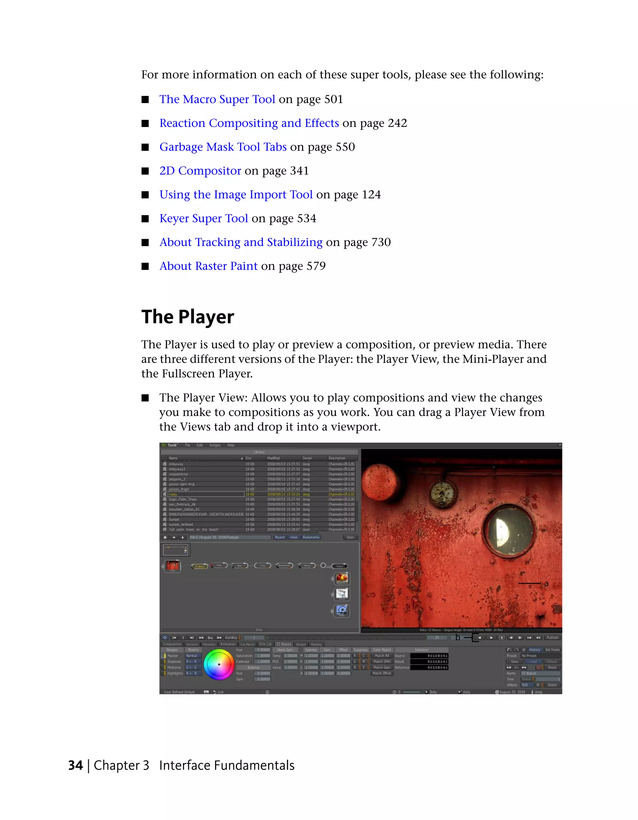
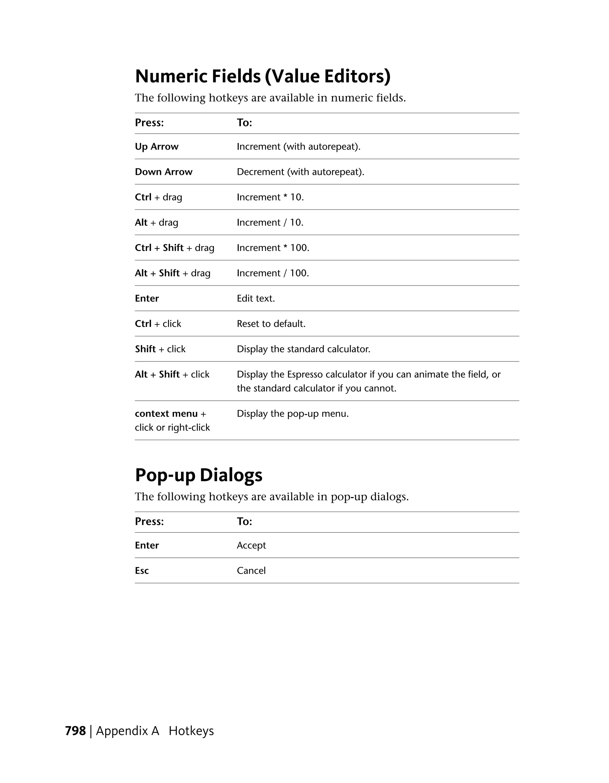
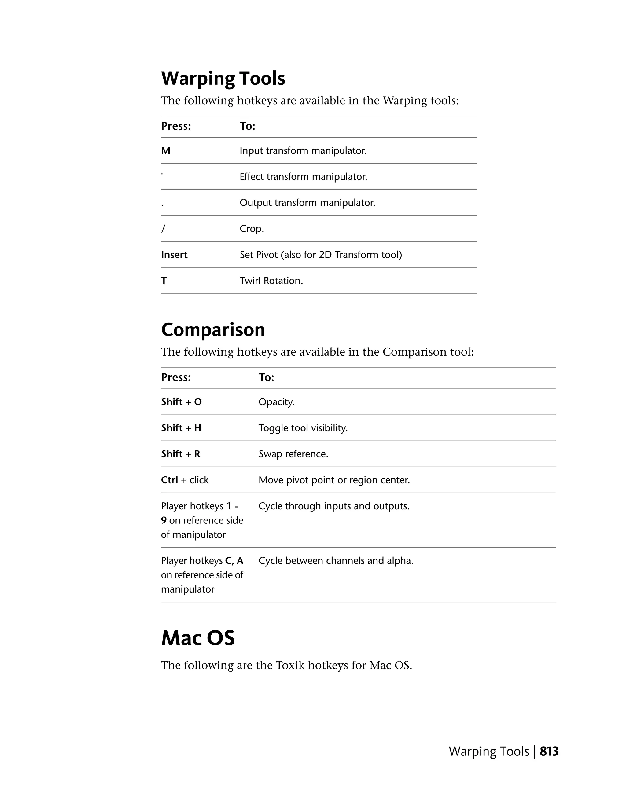
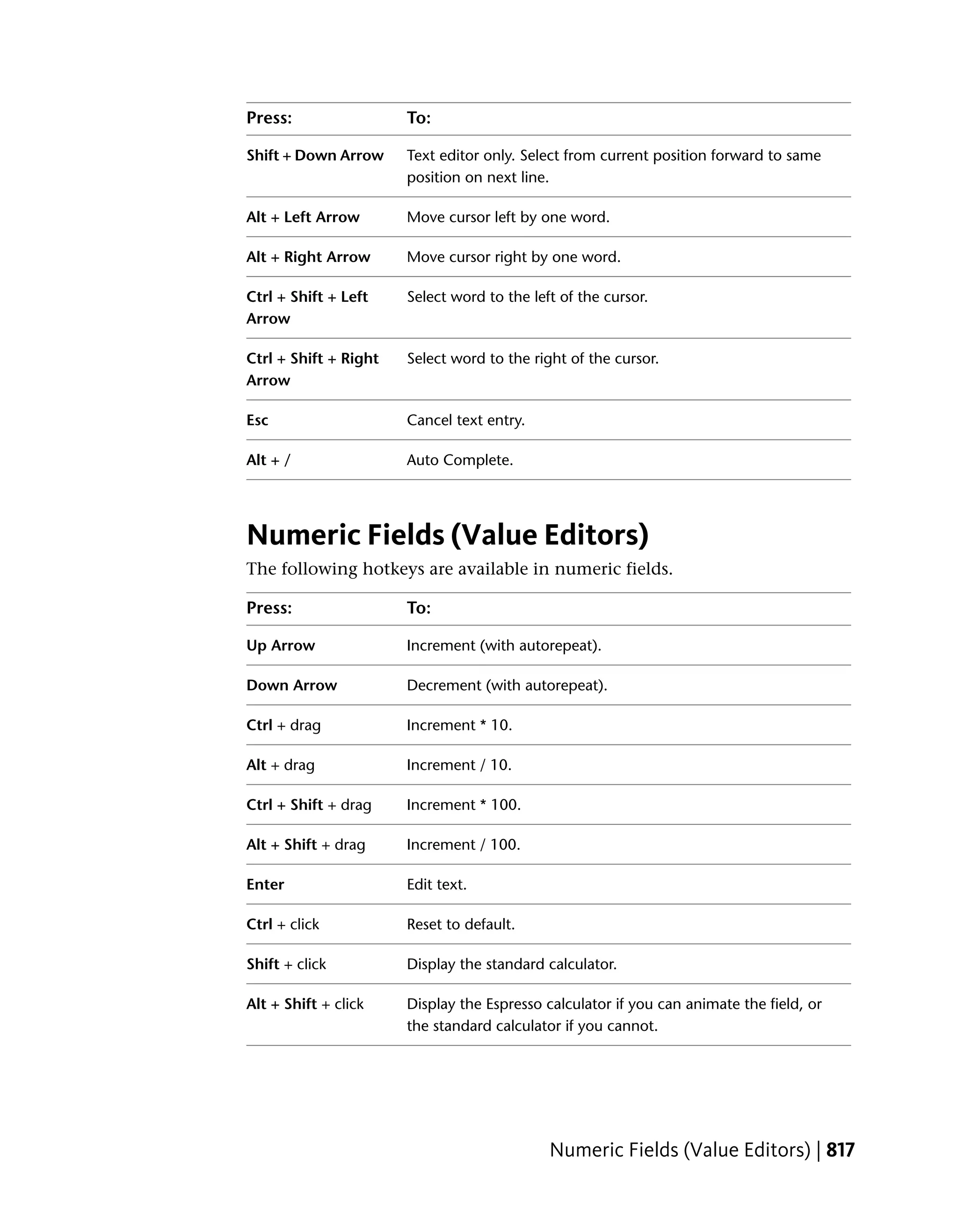
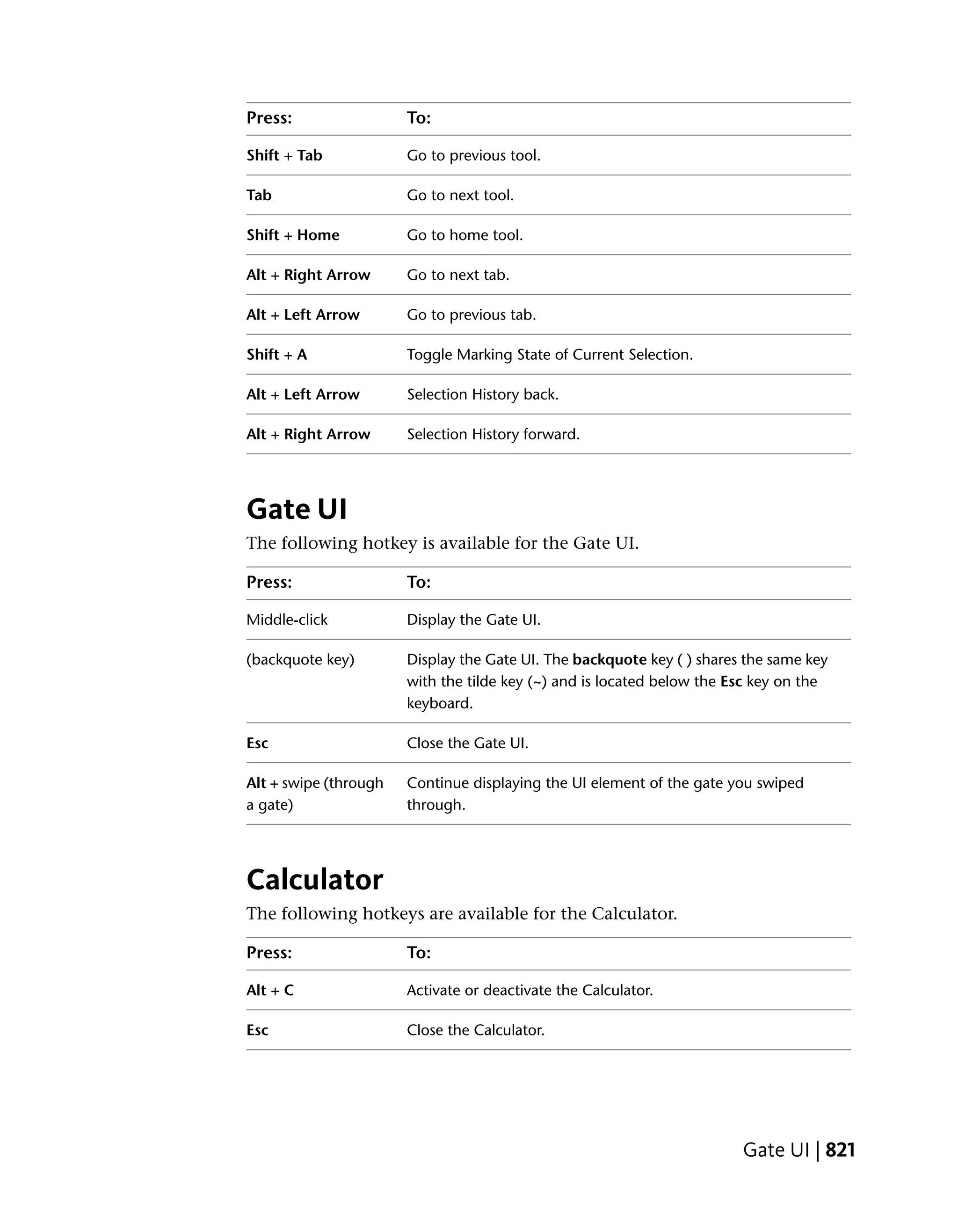
![Press: To:
9 Display rendered output.
Ctrl + R Reset nodes.
Shift + C Toggle Comparison tool.
Shift + D Toggle Display Modifier tool.
0 Next stream (stereo)
Shift + 0 Previous stream (stereo)
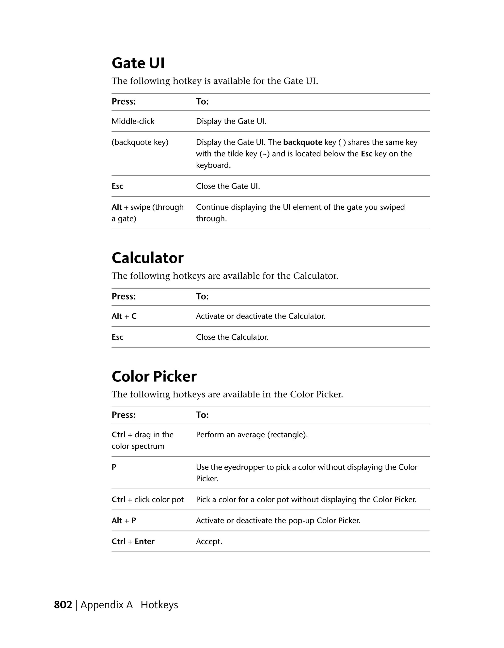
Separators
The following hotkey is available for manipulating UI separators.
Press: To:
Ctrl + click Reset to previous location.
Schematic
The following hotkeys are available in the Schematic view.
Press: To:
[1-4] + click a node Set a context point on that node. The number indicates the
number of the context point. For example, pressing 1 + click
sets context point 1. Pressing 3 + click sets context point 3.
[1-4] + click the Clear the context point. The number indicates the number of
background of the context point to clear. For example, pressing 2 + click clears
Schematic context point 2, and pressing 4 + click clears context point 4.
Shift + drag a node Connect the two nodes (Kiss). Release Shift and continue
into contact with an- dragging to cancel the operation.
other node
Alt + drag a node Insert the node between the two nodes joined by that connec-
onto a connection tion. Release Alt and continue dragging to cancel the operation.
806 | Appendix A Hotkeys](https://image.slidesharecdn.com/mayacompositeuserguide-1260452105-phpapp01/75/Mayacompositeuserguide-822-2048.jpg)
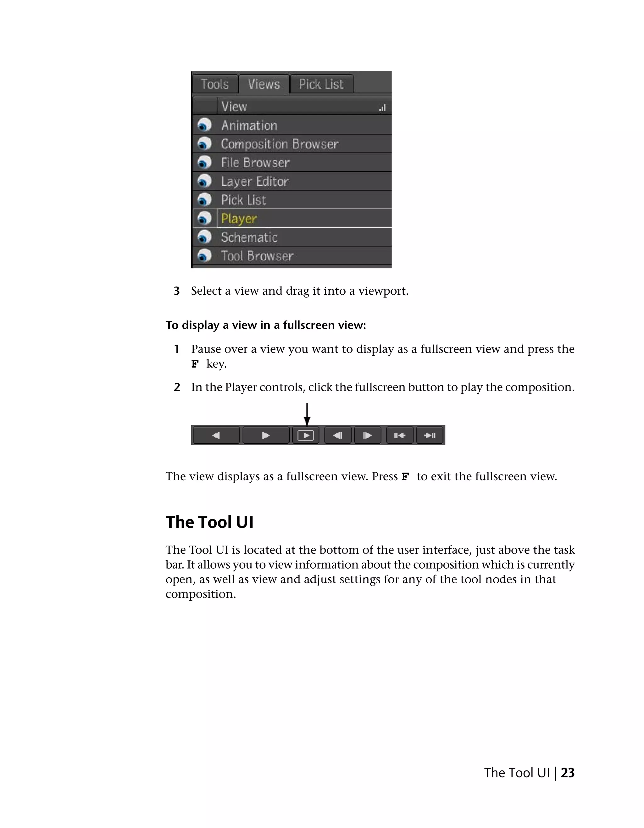
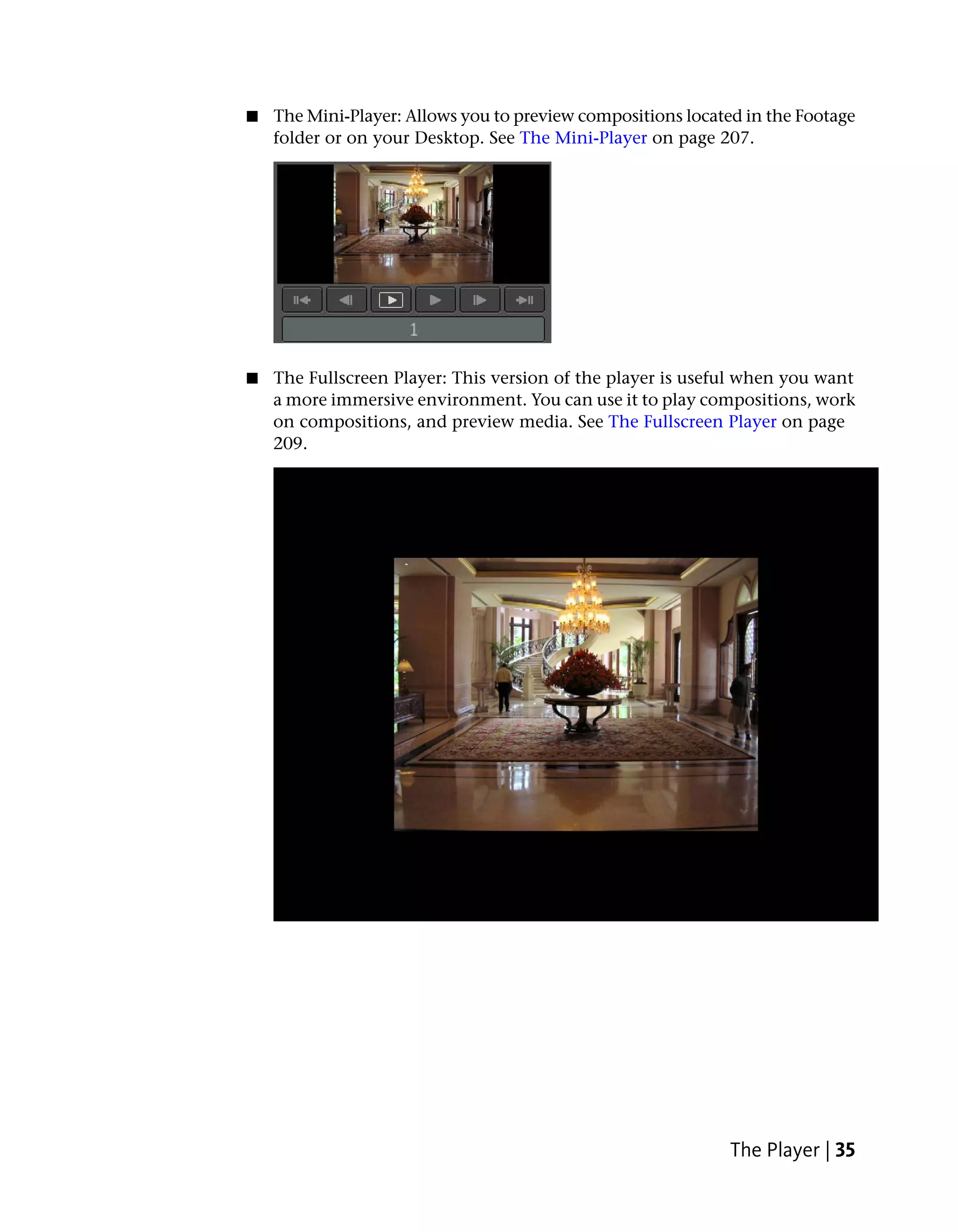
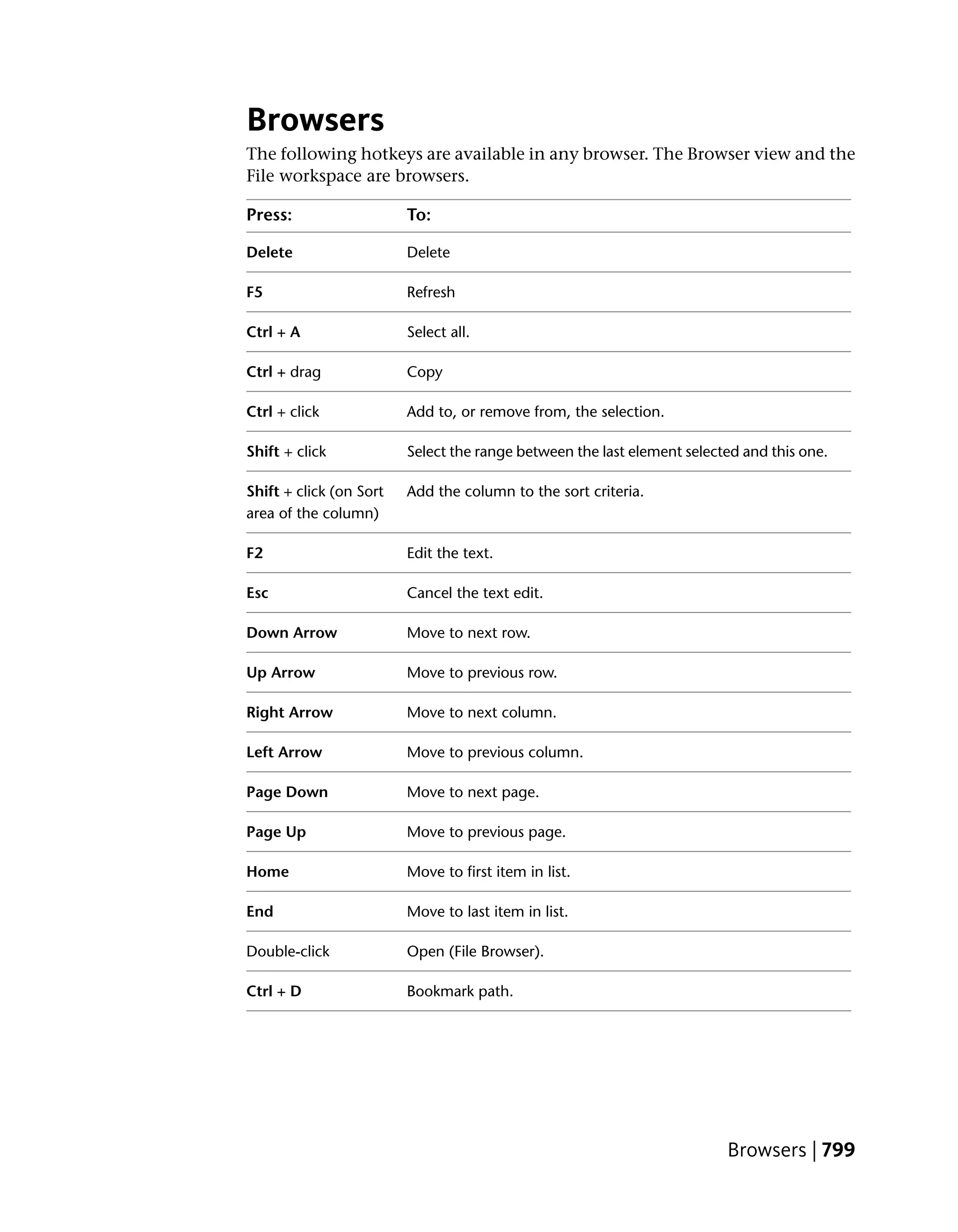
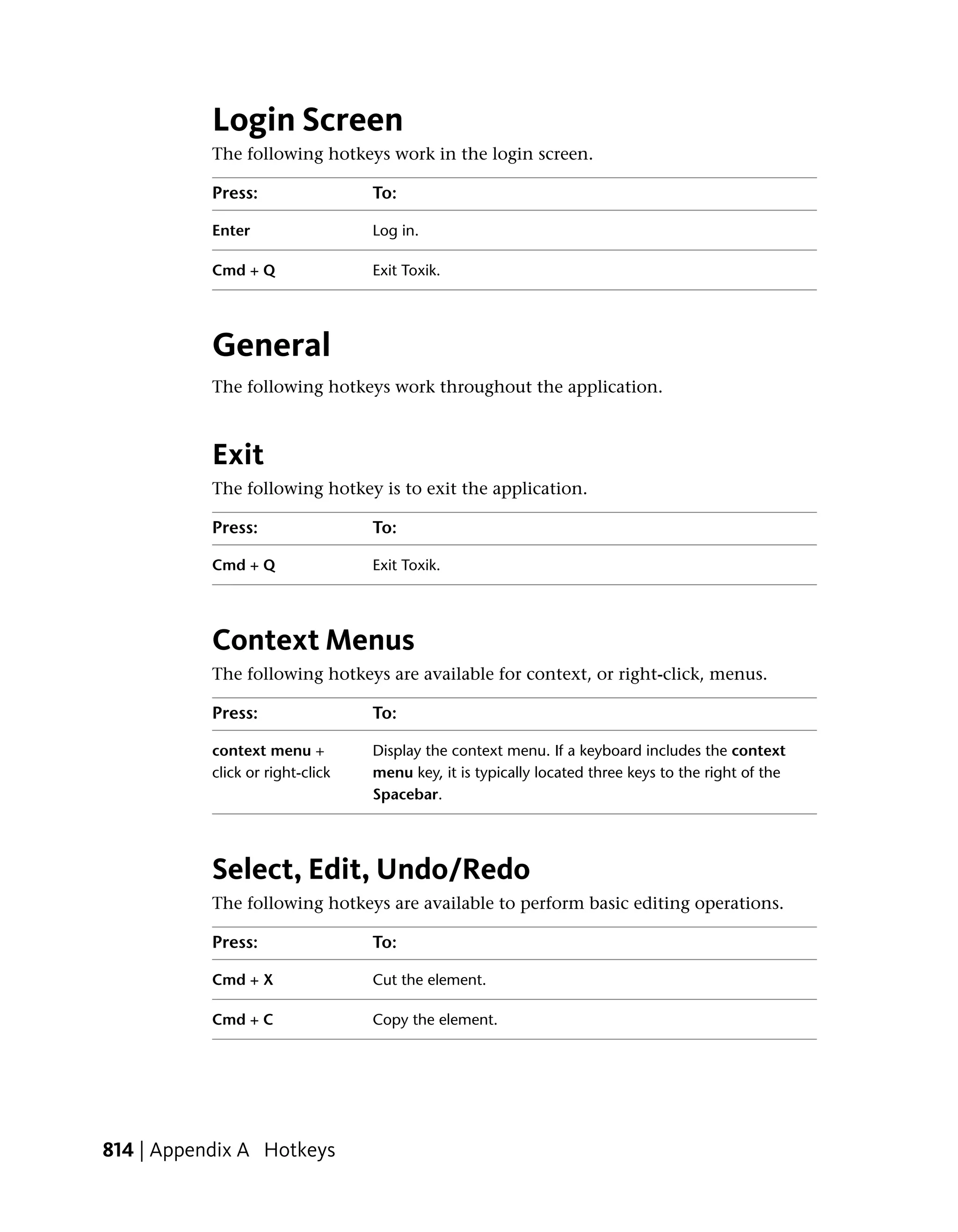
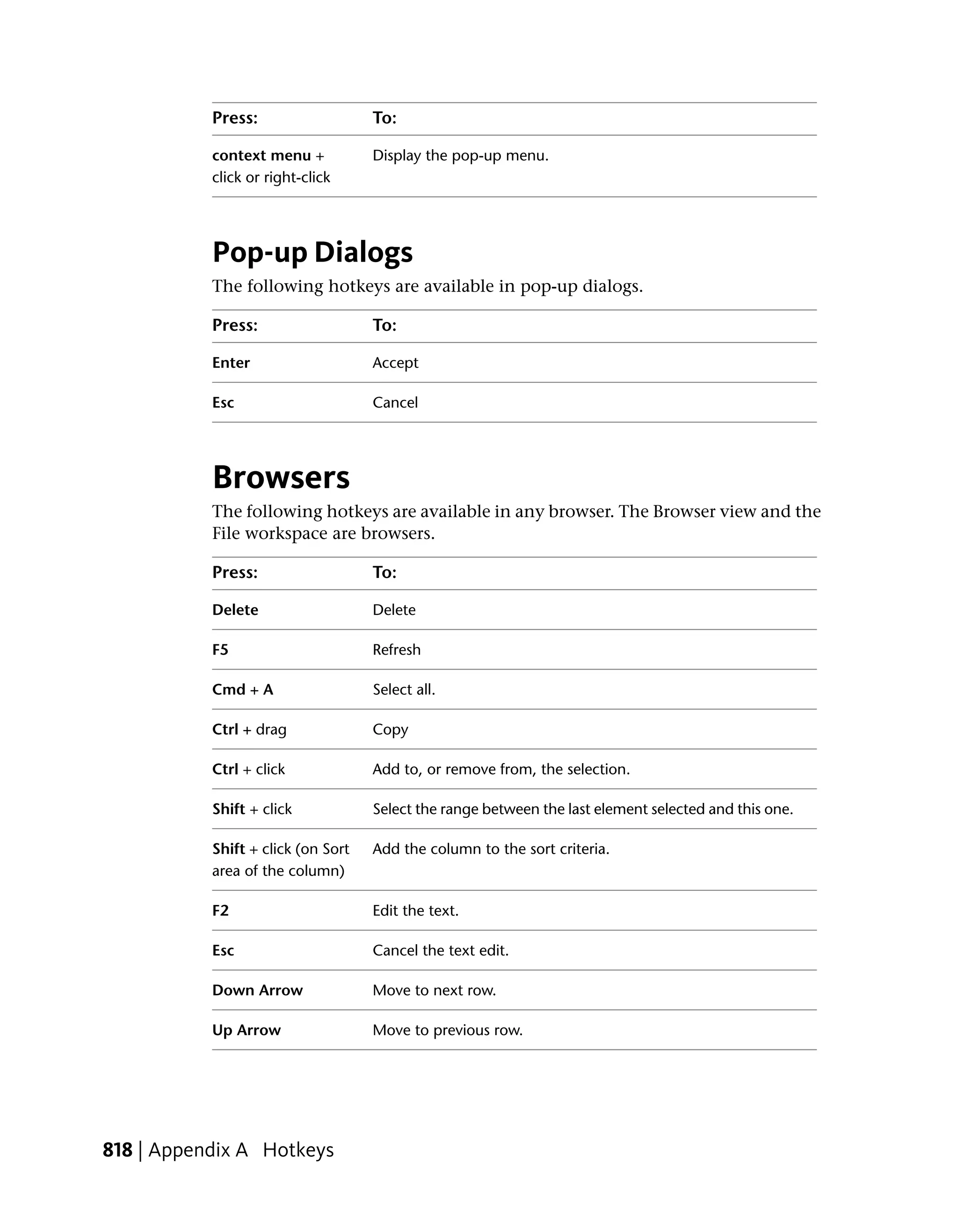
![Keyer
The following hotkeys are available in the Keyer tool.
Press: To:
M Sample matte.
Shift + [1-9] Sample patch [1-9].
D Sample degrain.
S Spill suppress.
Shift + B Adjust blend.
Master Keyer
The following hotkeys are available in the Master Keyer tool.
Press: To:
M Sample matte.
Shift + [1-9] Sample patch [1-9].
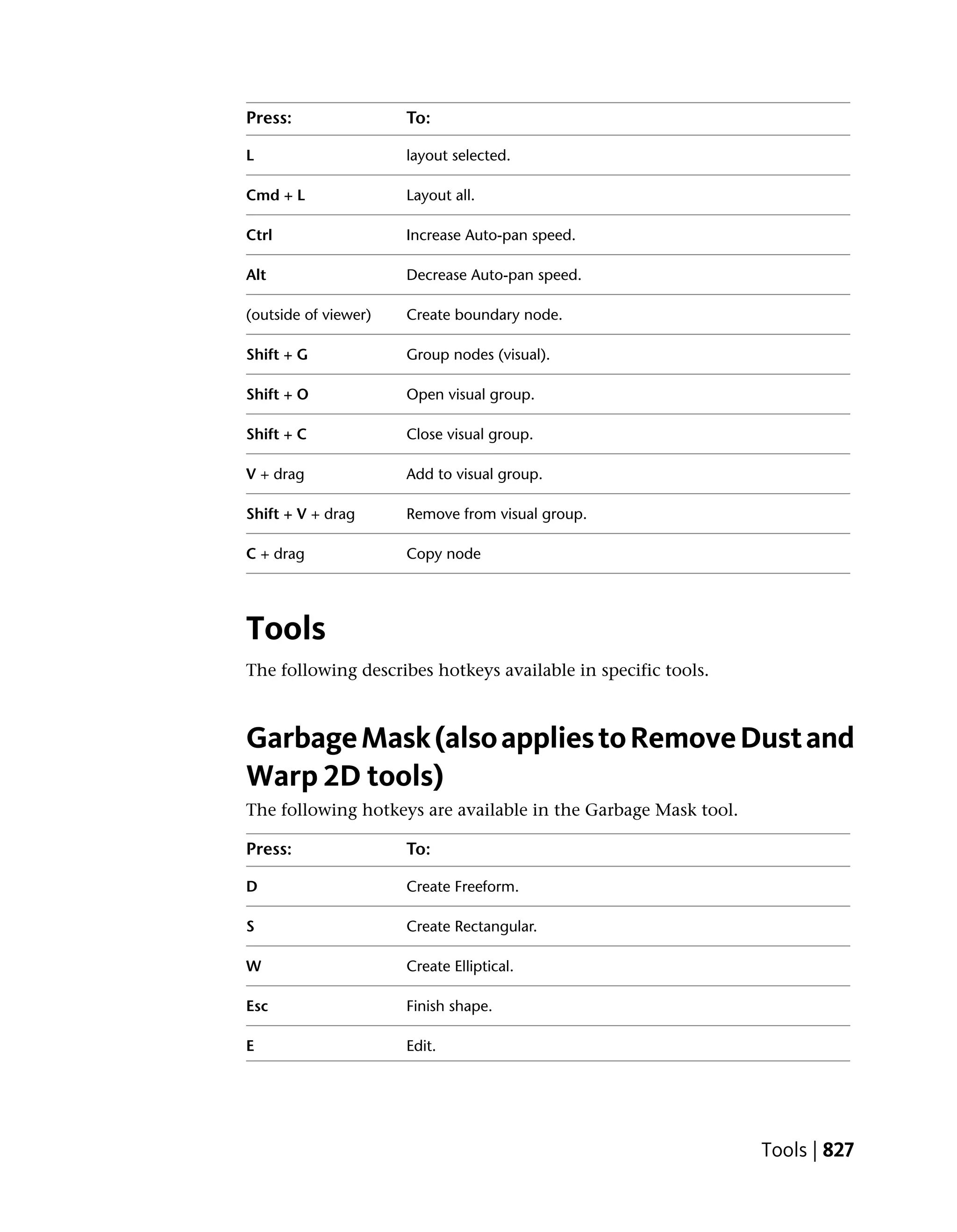
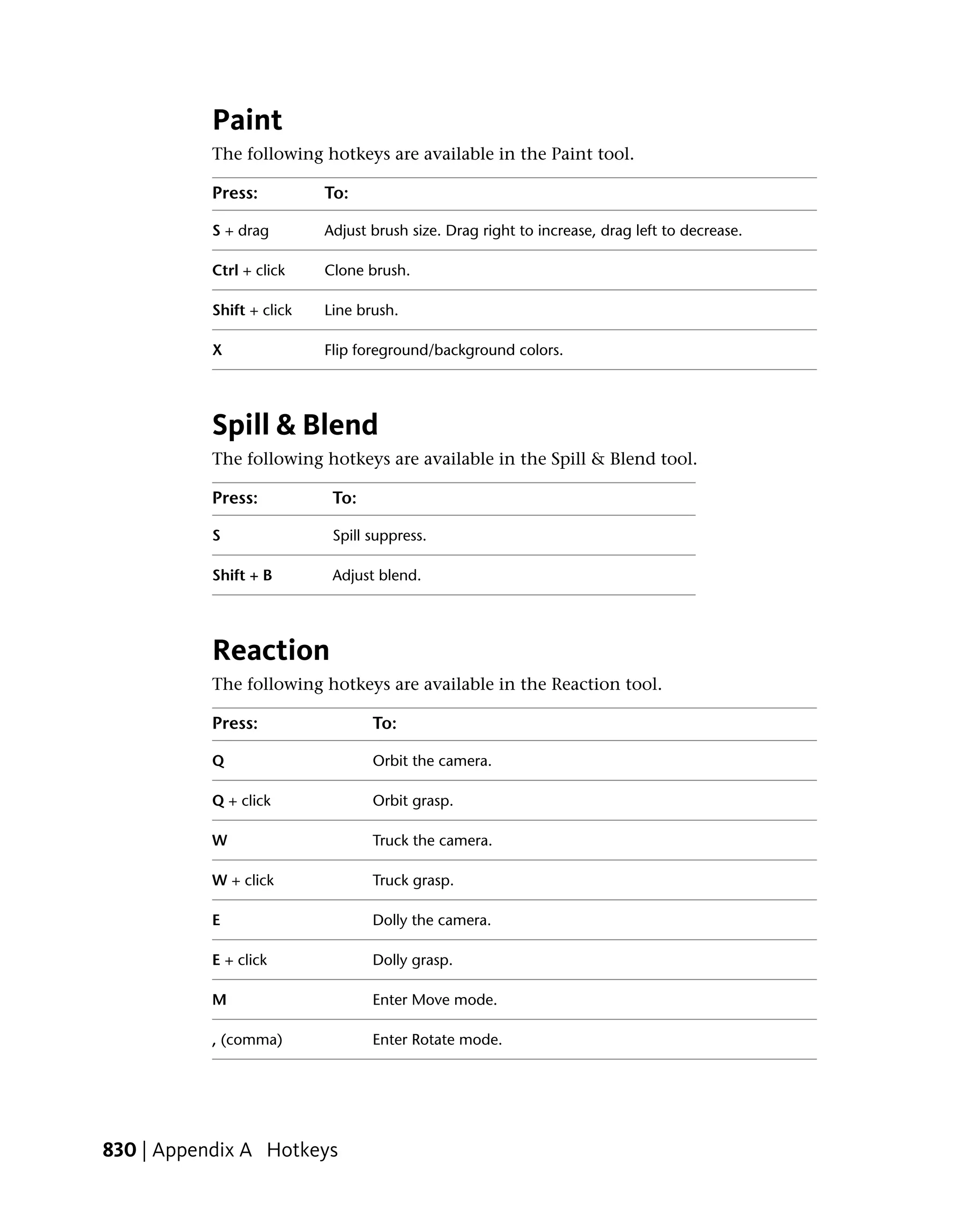
Paint
The following hotkeys are available in the Paint tool.
Press: To:
S + drag Adjust brush size. Drag right to increase, drag left to decrease.
Ctrl + click Clone brush.
Shift + click Line brush.
X Flip foreground/background colors.
810 | Appendix A Hotkeys](https://image.slidesharecdn.com/mayacompositeuserguide-1260452105-phpapp01/75/Mayacompositeuserguide-826-2048.jpg)
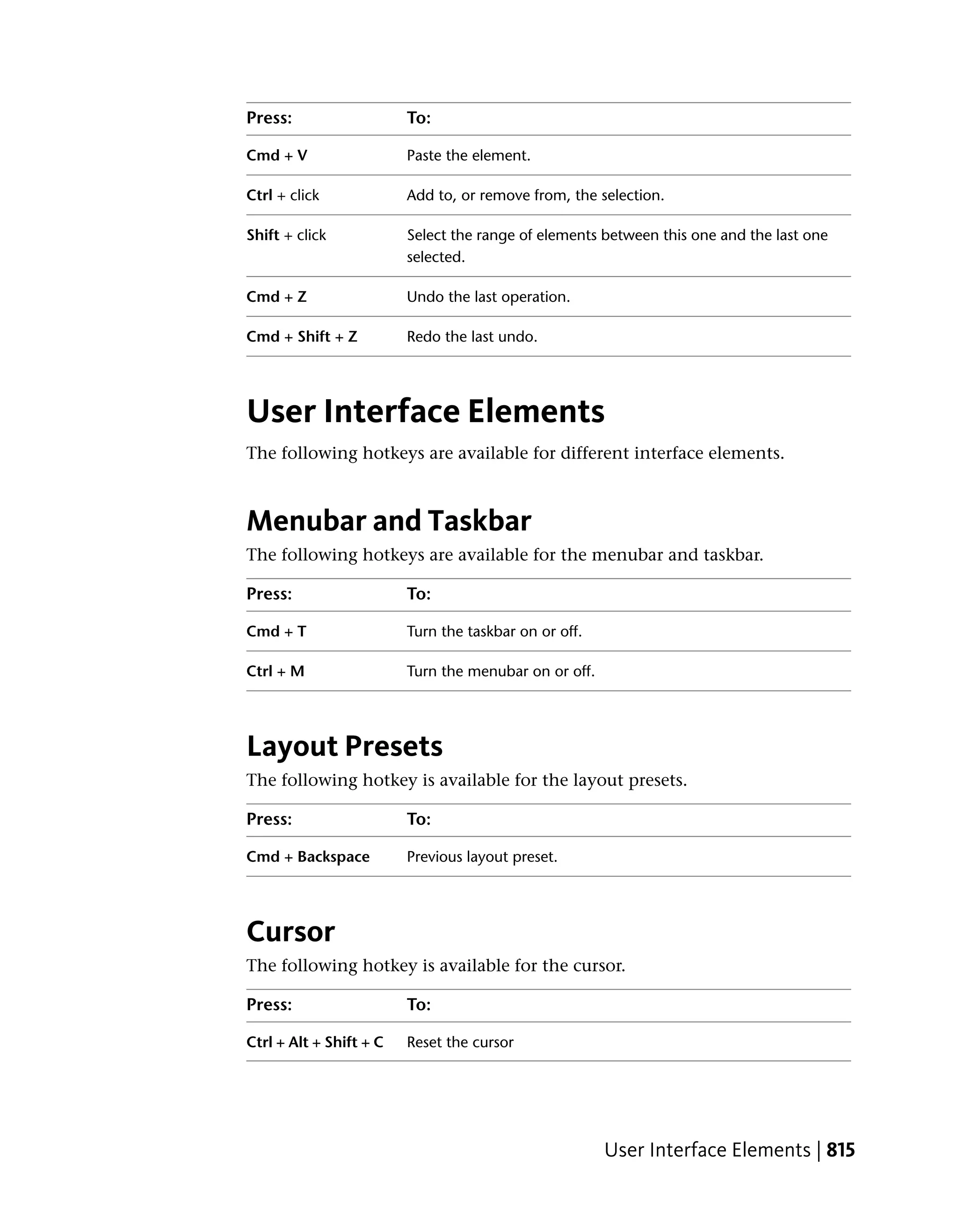
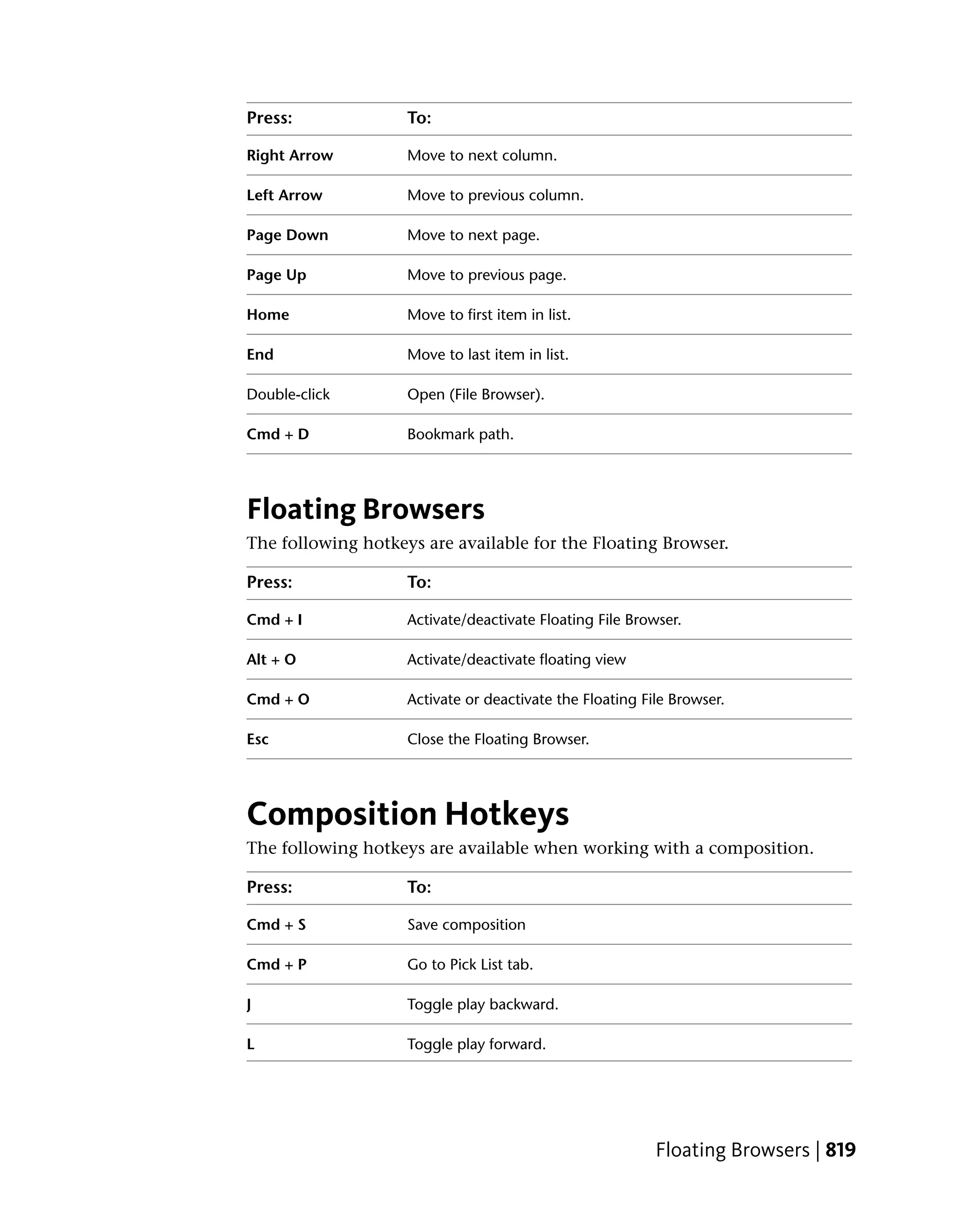
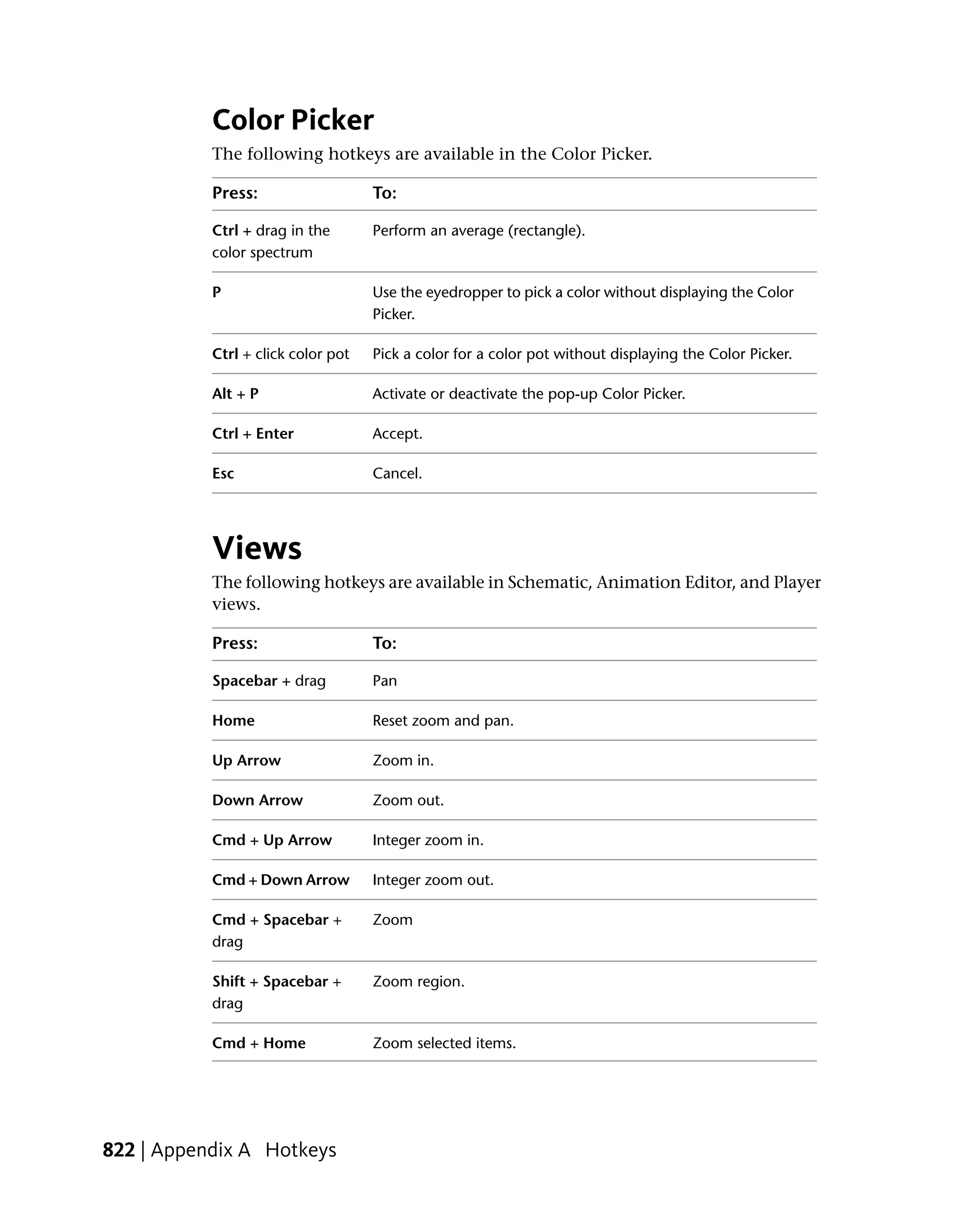
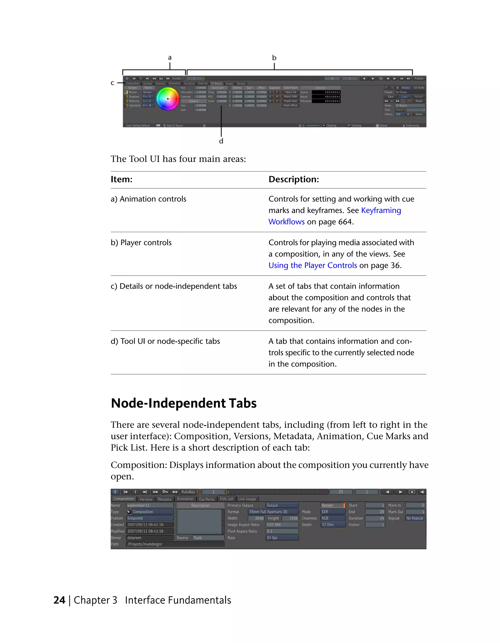
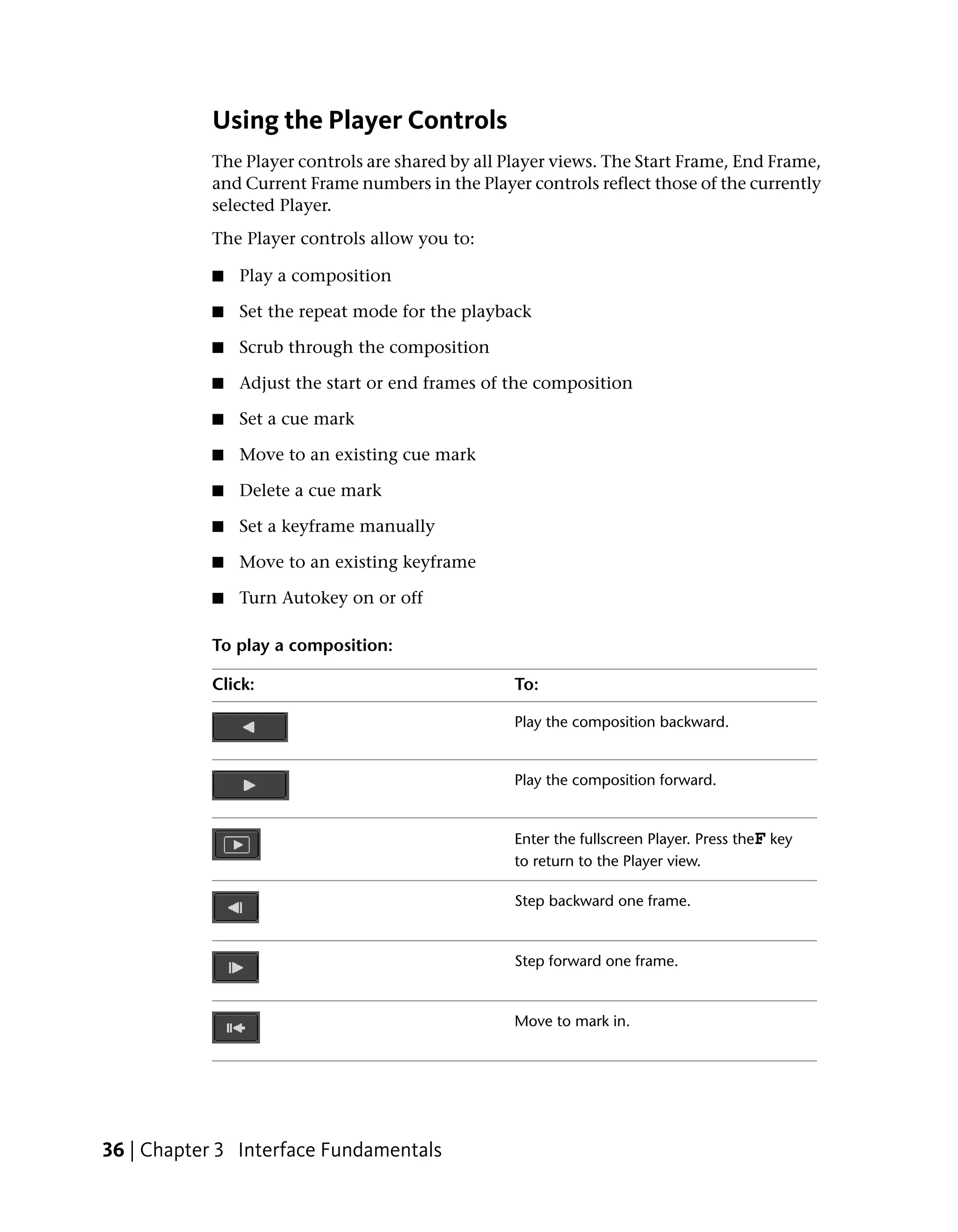
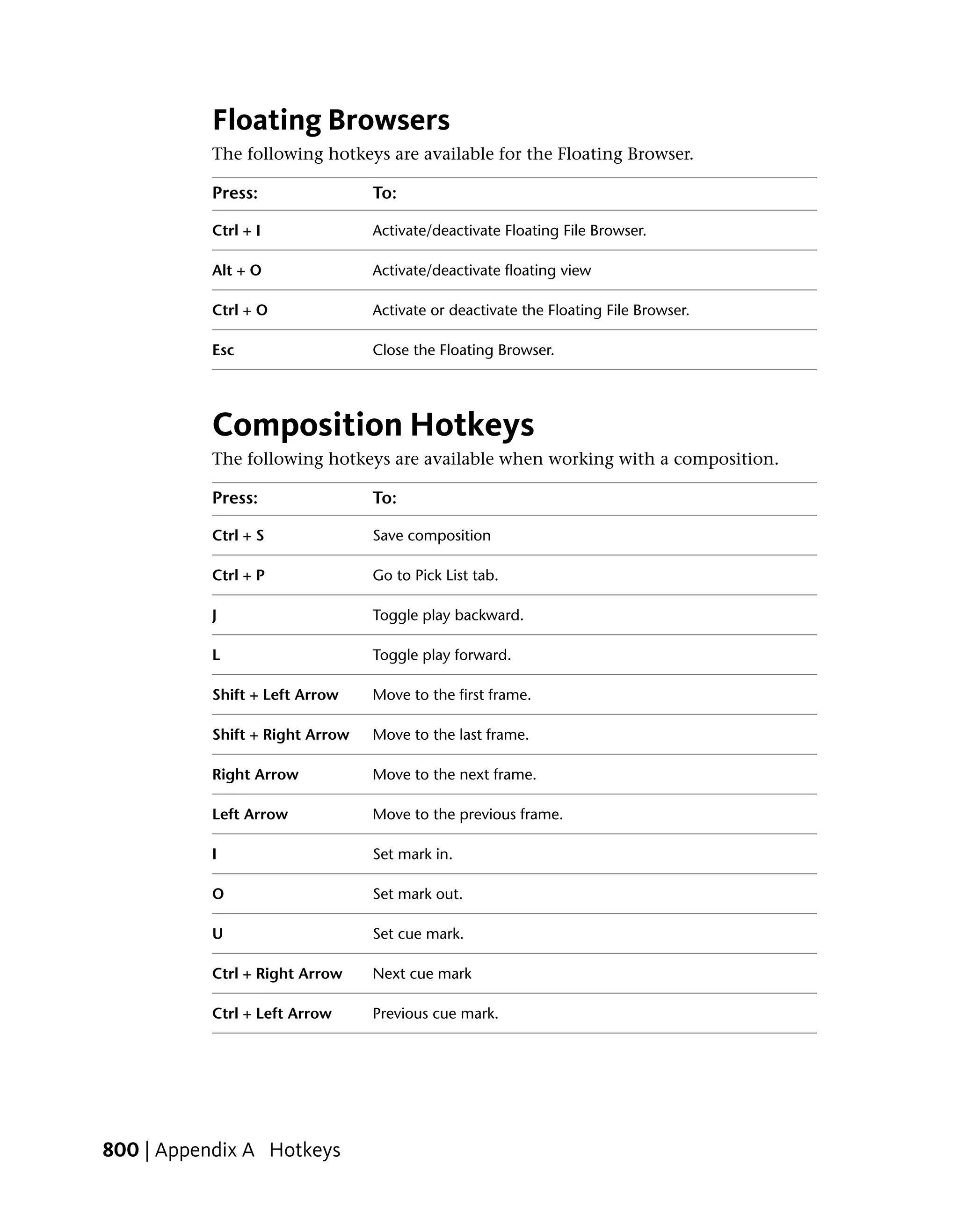
![Press: To:
Cmd + Alt + Home Zoom all scene.
[F1 - F4] Activate Viewpoint [1-4].
Cmd + [F1 - F4] Set Viewpoint [1-4].
Cmd + Shift + [F1 - Delete Viewpoint [1-4].
F4]
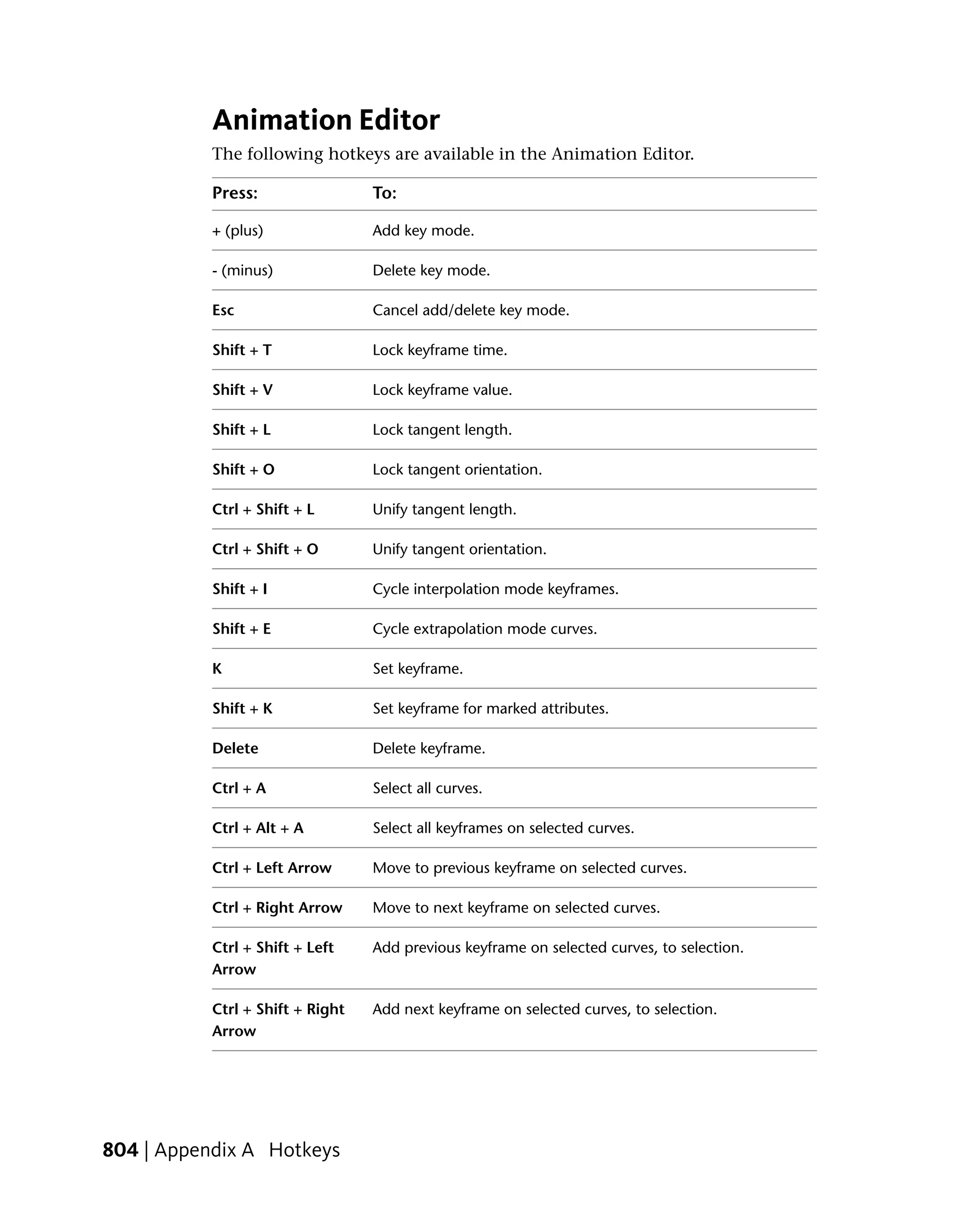
Animation Editor
The following hotkeys are available in the Animation Editor.
Press: To:
+ (plus) Add key mode.
- (minus) Delete key mode.
Esc Cancel add/delete key mode.
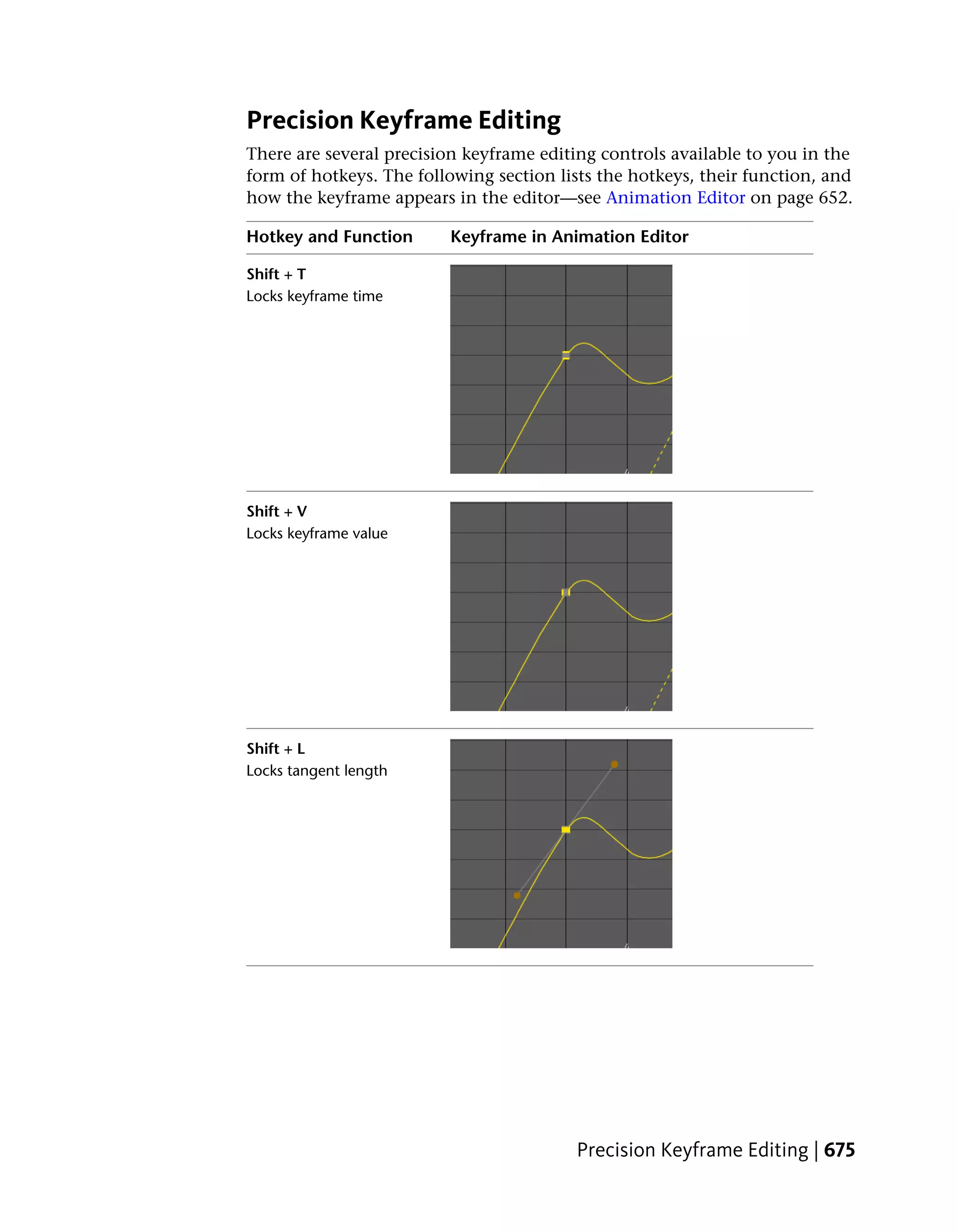
Shift + T Lock keyframe time.
Shift + V Lock keyframe value.
Shift + L Lock tangent length.
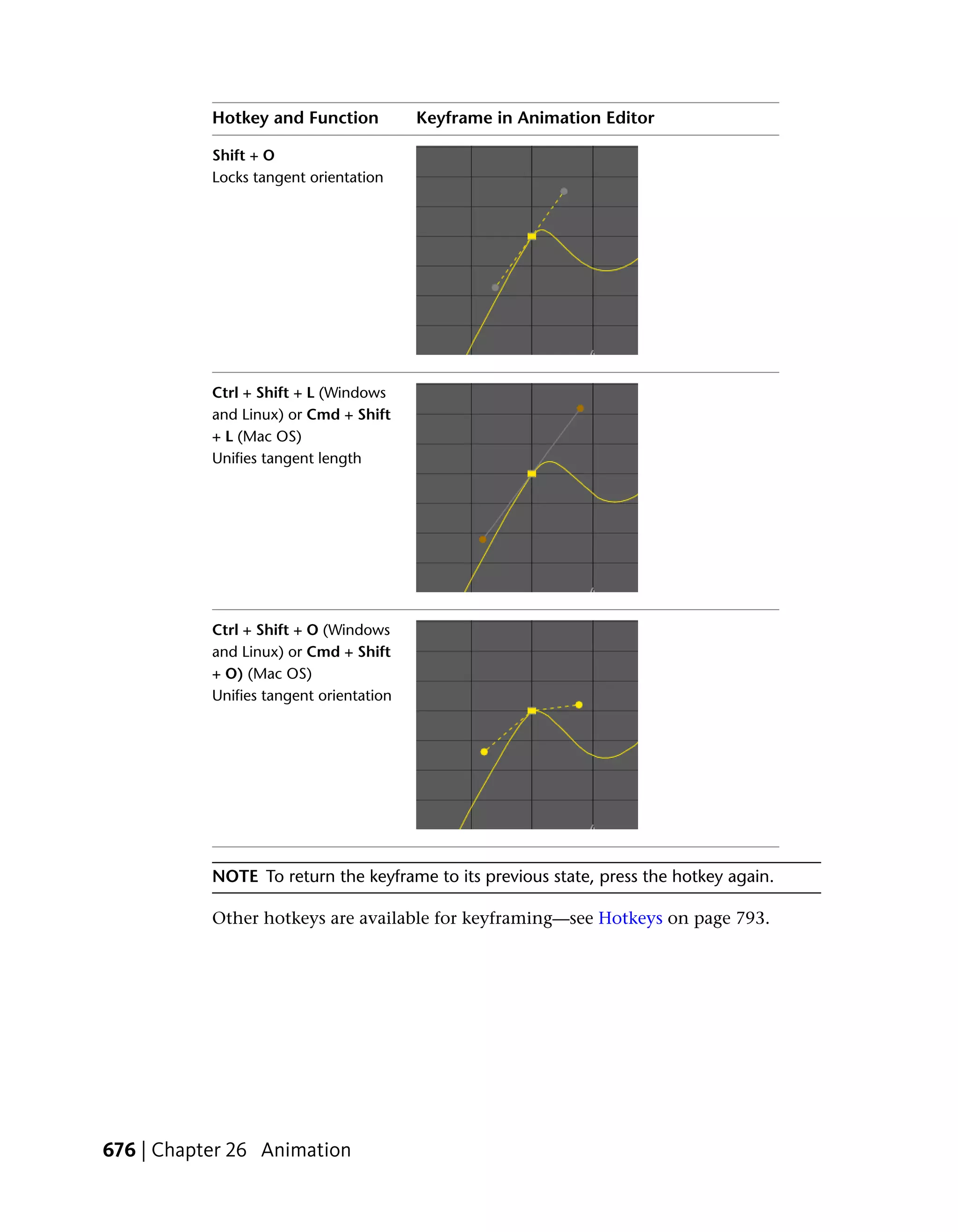
Shift + O Lock tangent orientation.
Cmd + Shift + L Unify tangent length.
Cmd + Shift + O Unify tangent orientation.
Shift + I Cycle interpolation mode keyframes.
Shift + E Cycle extrapolation mode curves.
K Set keyframe.
Shift + K Set keyframe for marked attributes.
Delete Delete keyframe.
Cmd + A Select all curves.
Animation Editor | 823](https://image.slidesharecdn.com/mayacompositeuserguide-1260452105-phpapp01/75/Mayacompositeuserguide-839-2048.jpg)
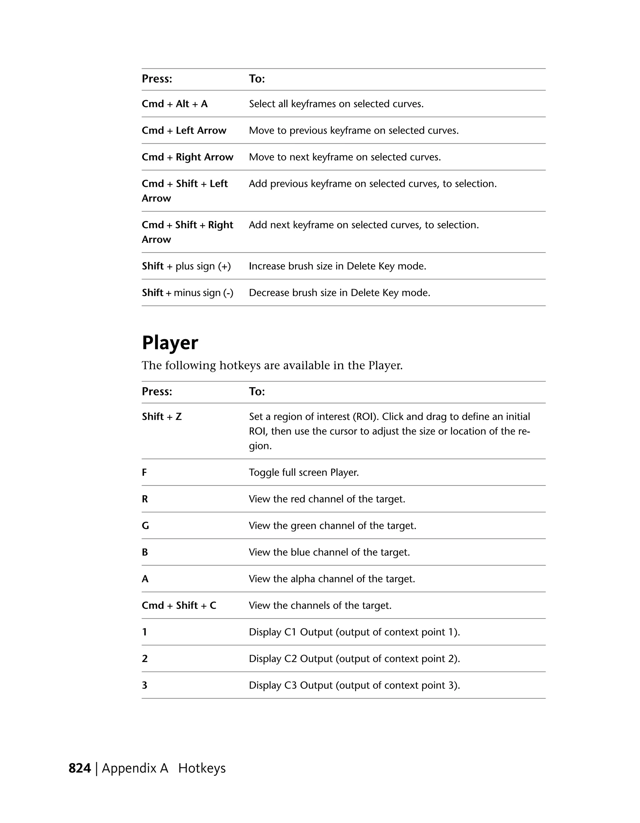
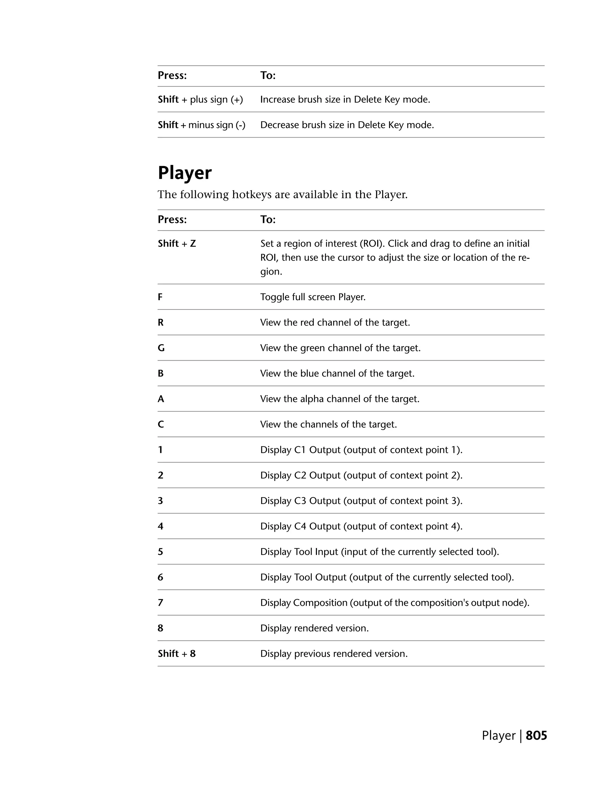
![Press: To:
4 Display C4 Output (output of context point 4).
5 Display Tool Input (input of the currently selected tool).
6 Display Tool Output (output of the currently selected tool).
7 Display Composition (output of the composition's output node).
8 Display rendered version.
Shift + 8 Display previous rendered version.
9 Display rendered output.
Cmd + Shift + R Reset nodes.
Shift + C Toggle Comparison tool.
Shift + D Toggle Display Modifier tool.
0 Next stream (stereo)
Shift + 0 Previous stream (stereo)
Separators
The following hotkey is available for manipulating UI separators.
Press: To:
Ctrl + click Reset to previous location.
Schematic
The following hotkeys are available in the Schematic view.
Press: To:
[1-4] + click a node Set a context point on that node. The number indicates the
number of the context point. For example, pressing 1 + click
sets context point 1. Pressing 3 + click sets context point 3.
Separators | 825](https://image.slidesharecdn.com/mayacompositeuserguide-1260452105-phpapp01/75/Mayacompositeuserguide-841-2048.jpg)
![Press: To:
[1-4] + click the Clear the context point. The number indicates the number of
background of the context point to clear. For example, pressing 2 + click clears
Schematic context point 2, and pressing 4 + click clears context point 4.
Shift + drag a node Connect the two nodes (Kiss). Release Shift and continue
into contact with an- dragging to cancel the operation.
other node
Alt + drag a node Insert the node between the two nodes joined by that connec-
onto a connection tion. Release Alt and continue dragging to cancel the operation.
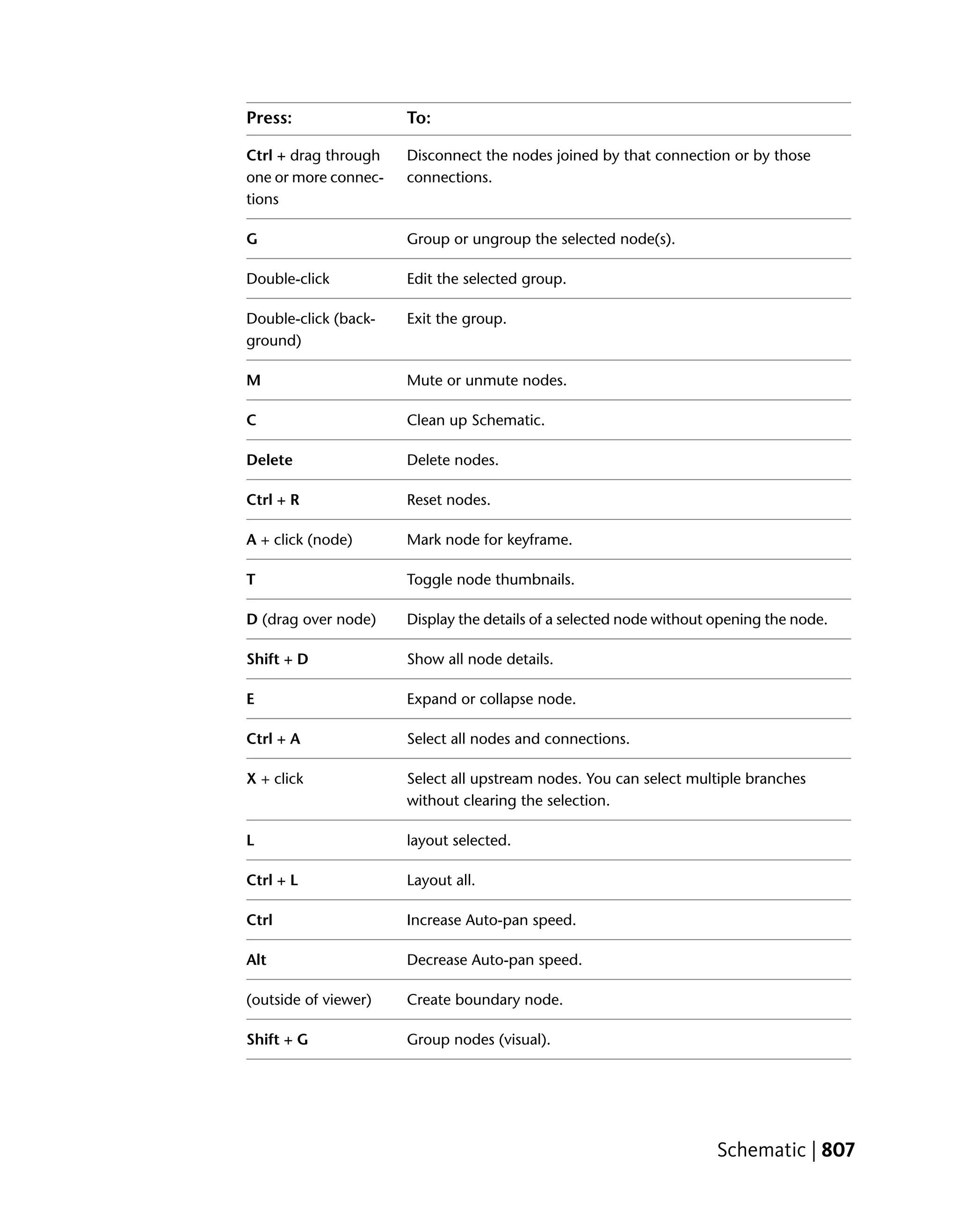
Cmd + drag through Disconnect the nodes joined by that connection or by those
one or more connec- connections.
tions
G Group or ungroup the selected node(s).
Double-click Edit the selected group.
Double-click (back- Exit the group.
ground)
M Mute or unmute nodes.
C Clean up Schematic.
Delete Delete nodes.
Ctrl + R Reset nodes.
A + click (node) Mark node for keyframe.
T Toggle node thumbnails.
D (drag over node) Display the details of a selected node without opening the node.
Shift + D Show all node details.
E Expand or collapse node.
Cmd + A Select all nodes and connections.
X + click Select all upstream nodes. You can select multiple branches
without clearing the selection.
826 | Appendix A Hotkeys](https://image.slidesharecdn.com/mayacompositeuserguide-1260452105-phpapp01/75/Mayacompositeuserguide-842-2048.jpg)
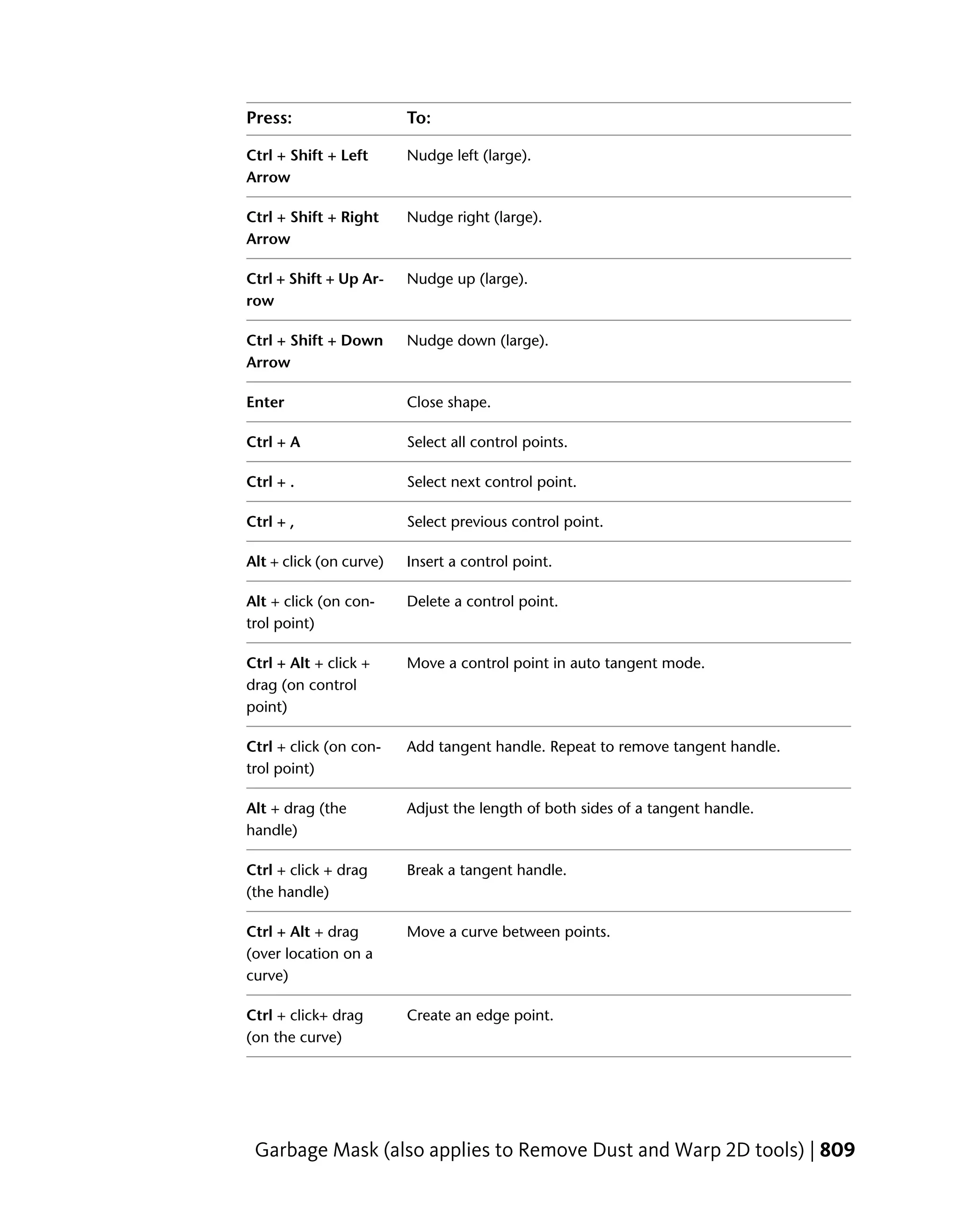
![Press: To:
Ctrl + click + drag Break a tangent handle.
(the handle)
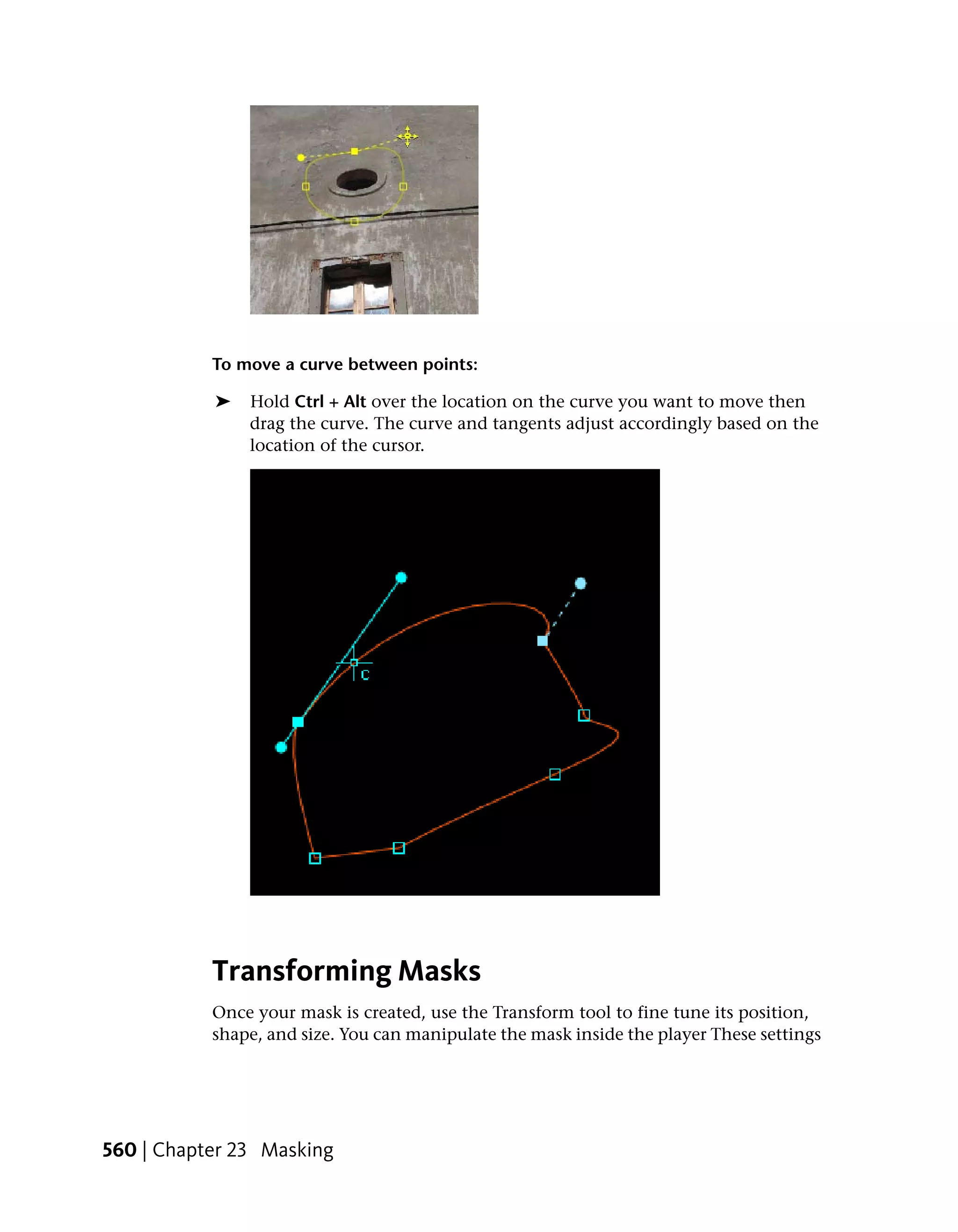
Ctrl + Alt + drag Move a curve between points.
(over location on a
curve)
Ctrl + click+ drag Create an edge point.
(on the curve)
Keyer
The following hotkeys are available in the Keyer tool.
Press: To:
M Sample matte.
Shift + [1-9] Sample patch [1-9].
D Sample degrain.
S Spill suppress.
Shift + B Adjust blend.
Master Keyer
The following hotkeys are available in the Master Keyer tool.
Press: To:
M Sample matte.
Shift + [1-9] Sample patch [1-9].
Keyer | 829](https://image.slidesharecdn.com/mayacompositeuserguide-1260452105-phpapp01/75/Mayacompositeuserguide-845-2048.jpg)


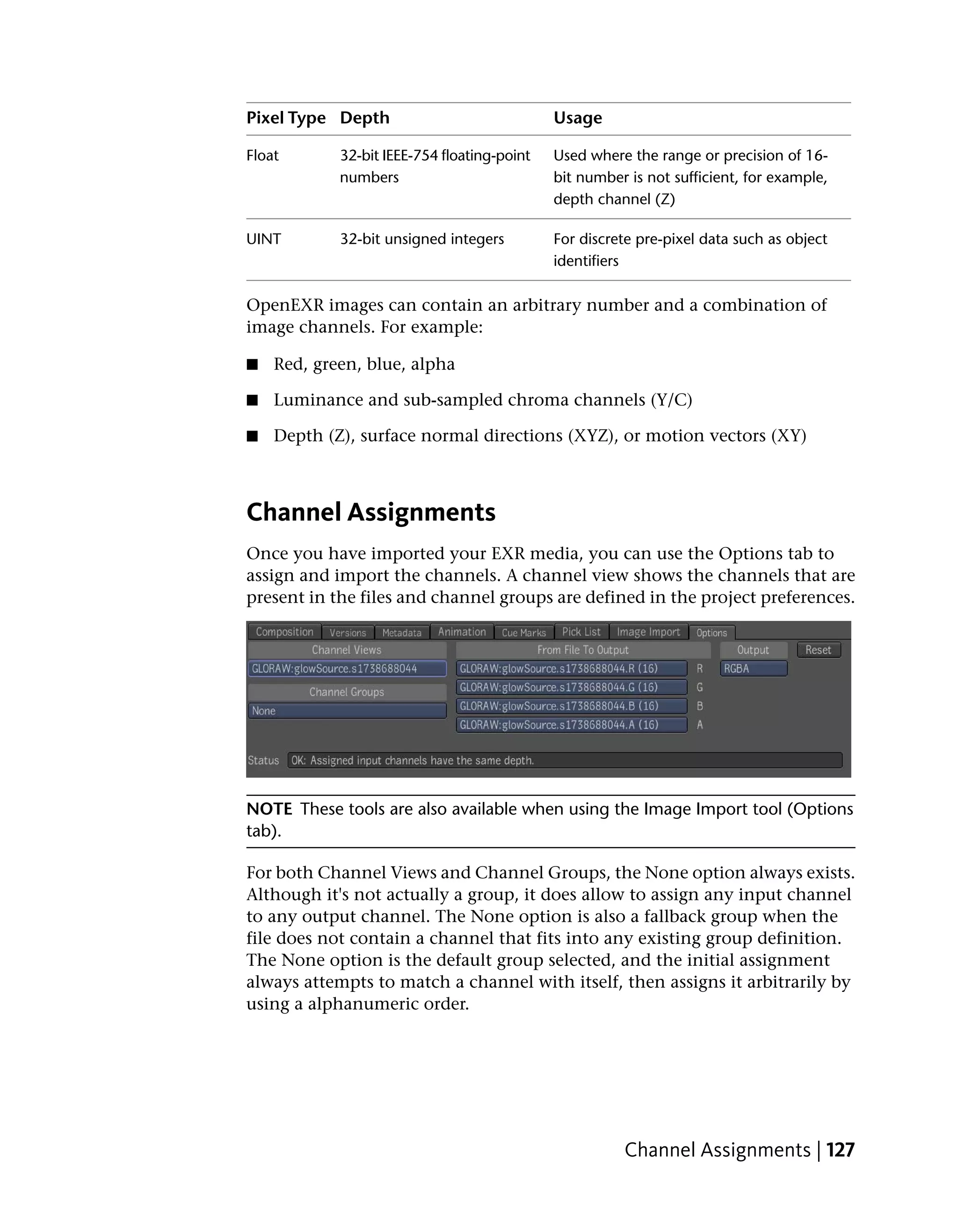
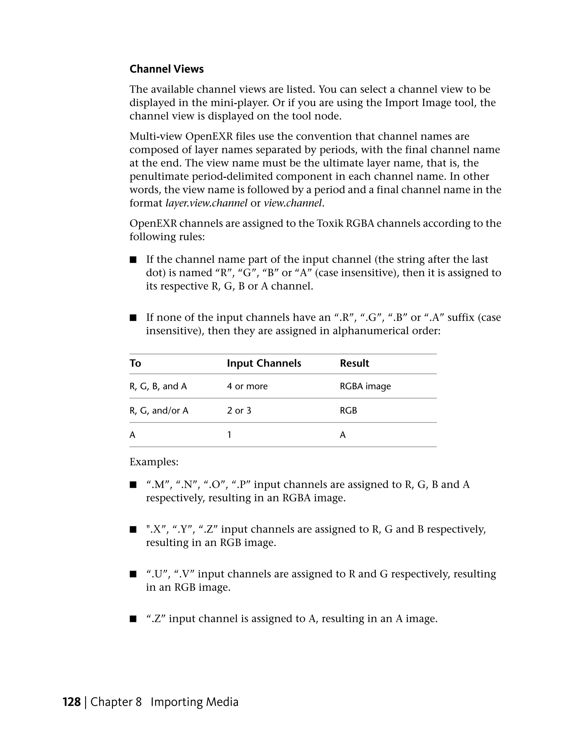
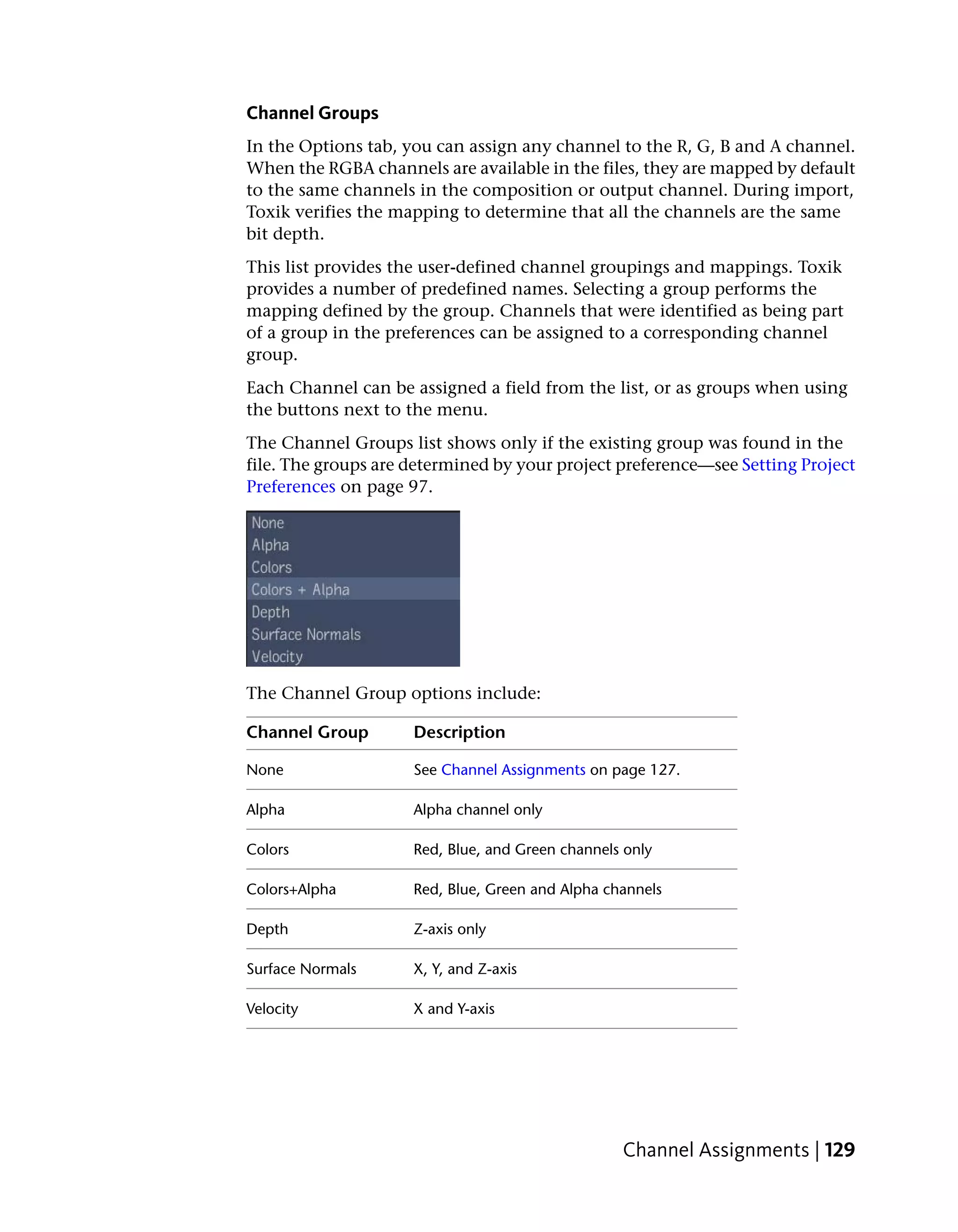
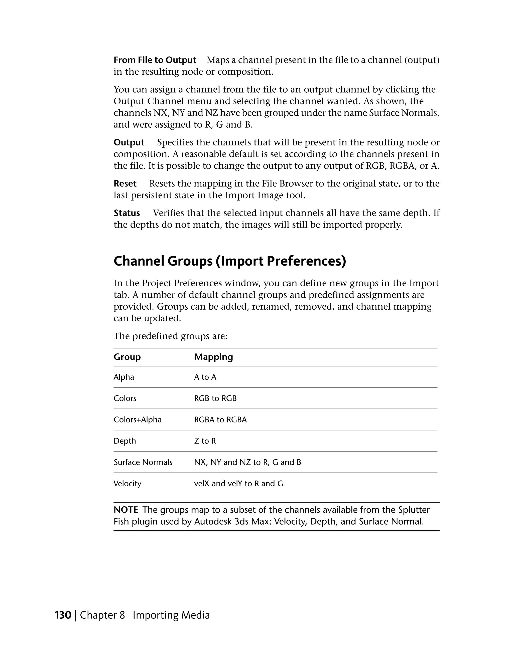
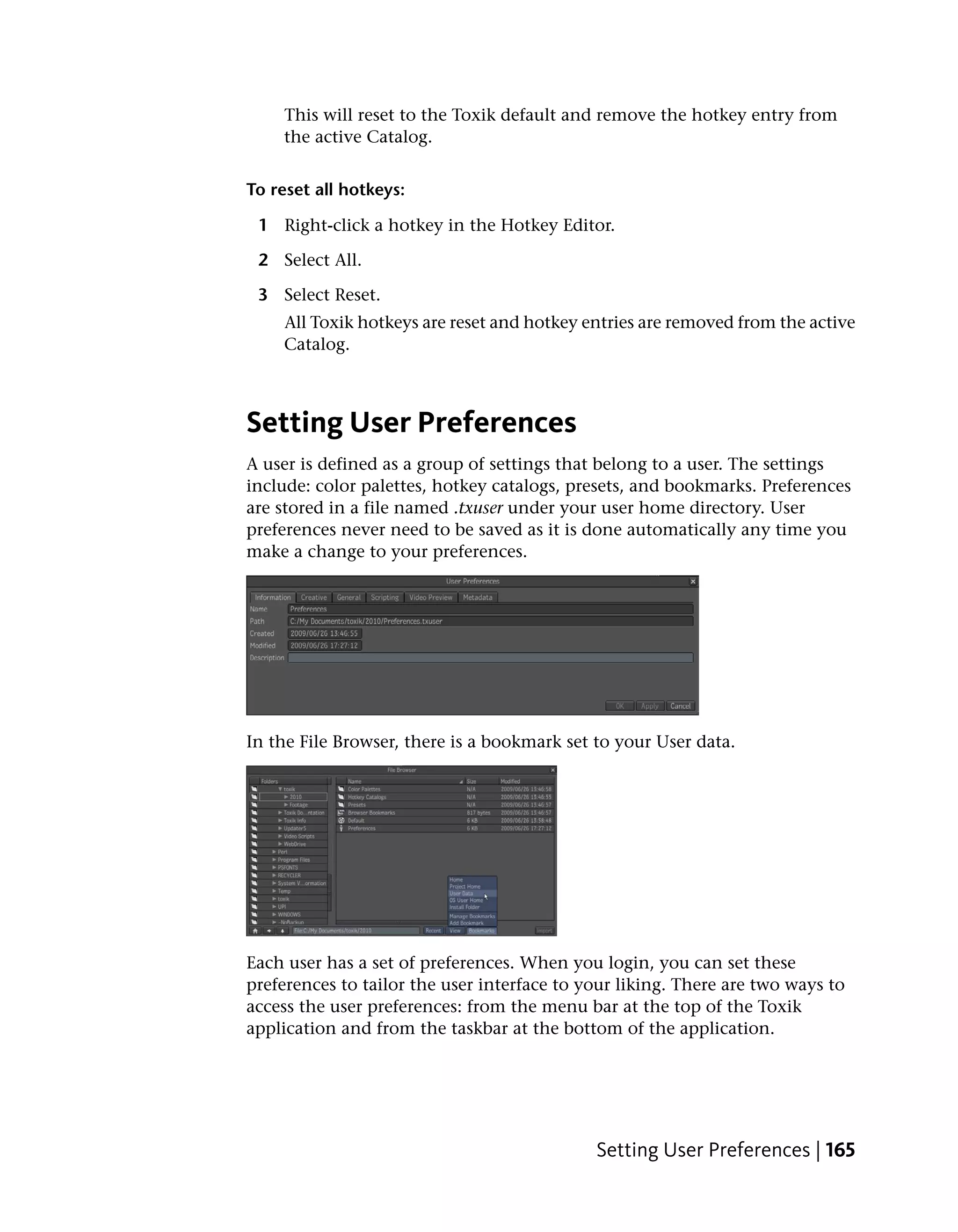
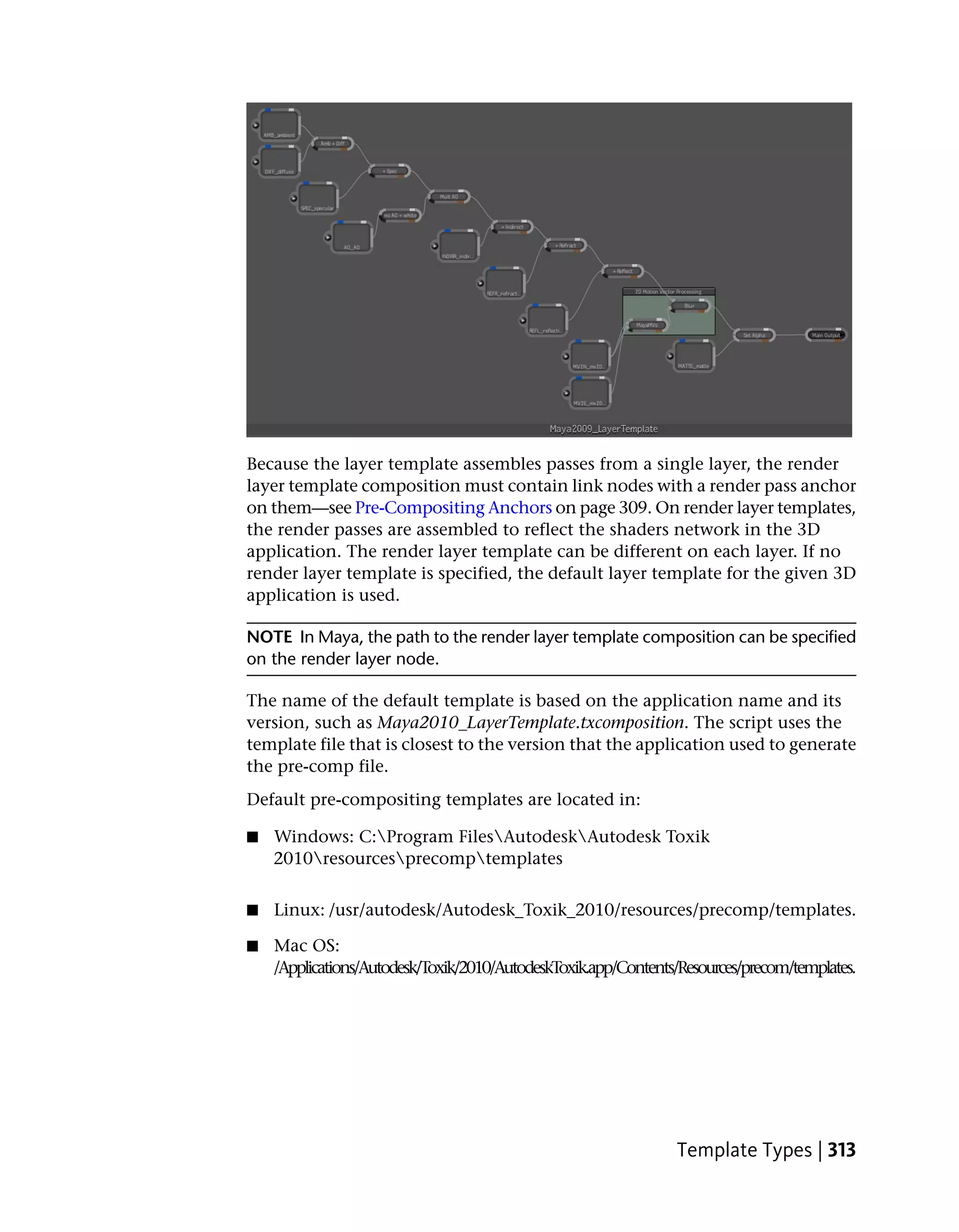
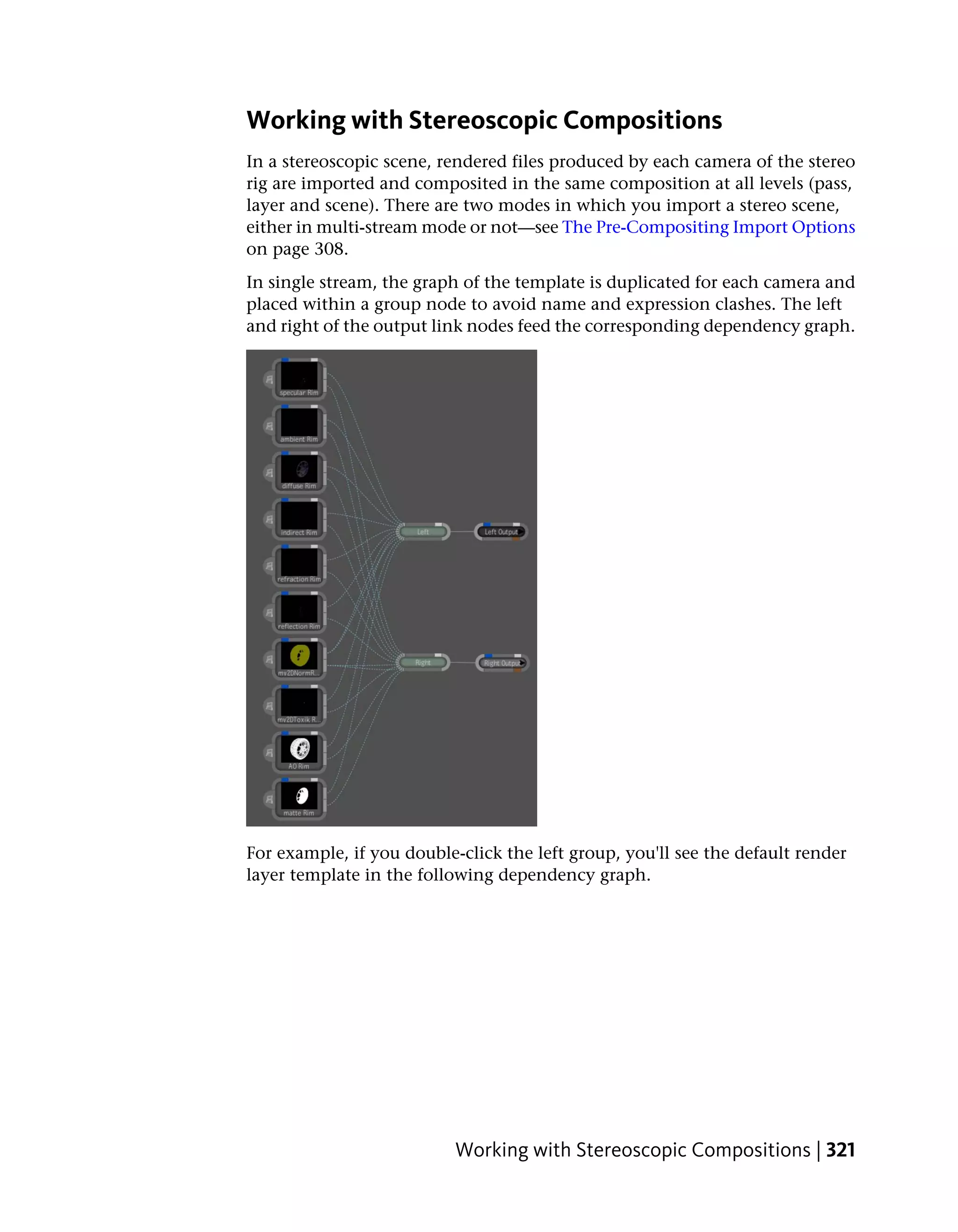
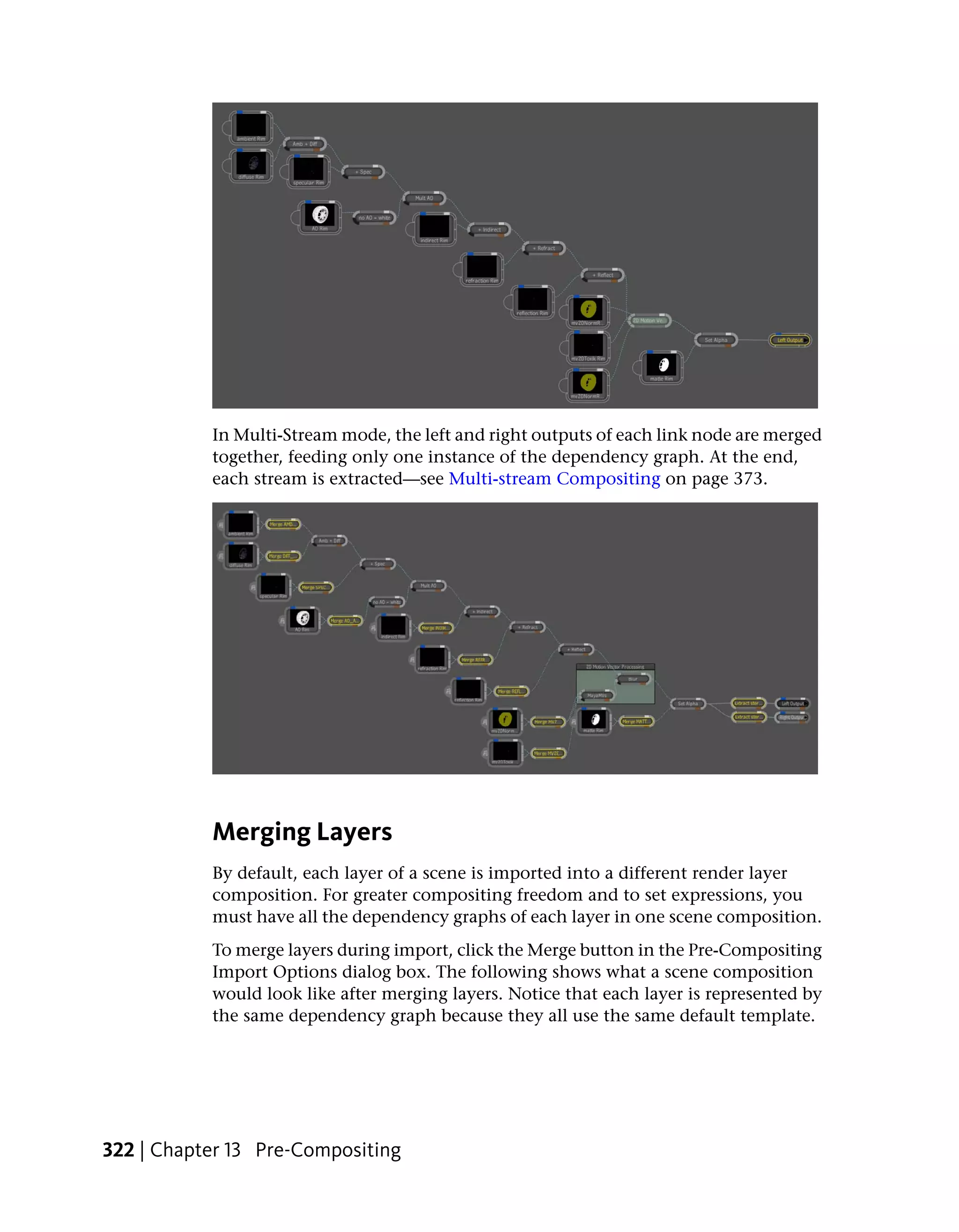
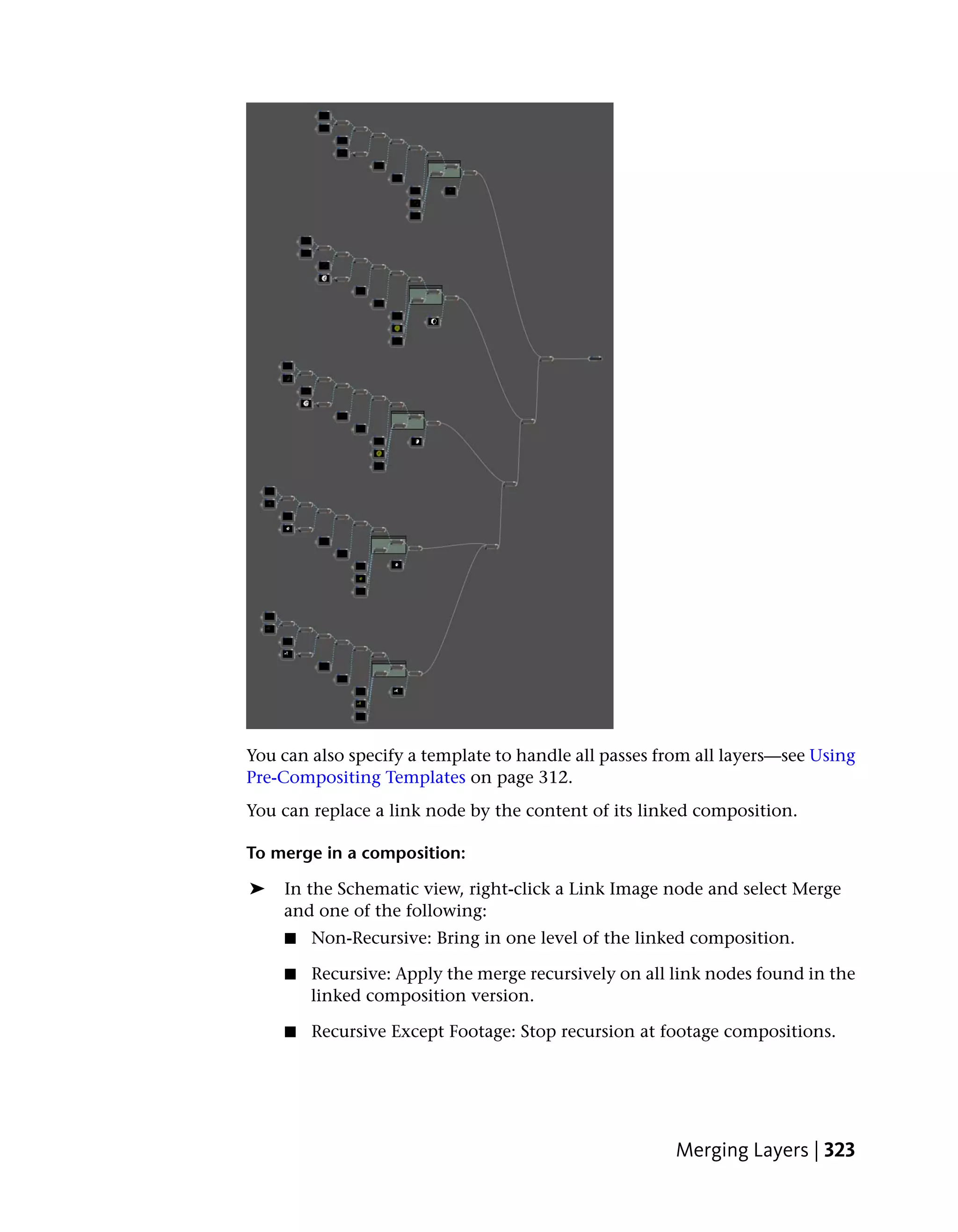
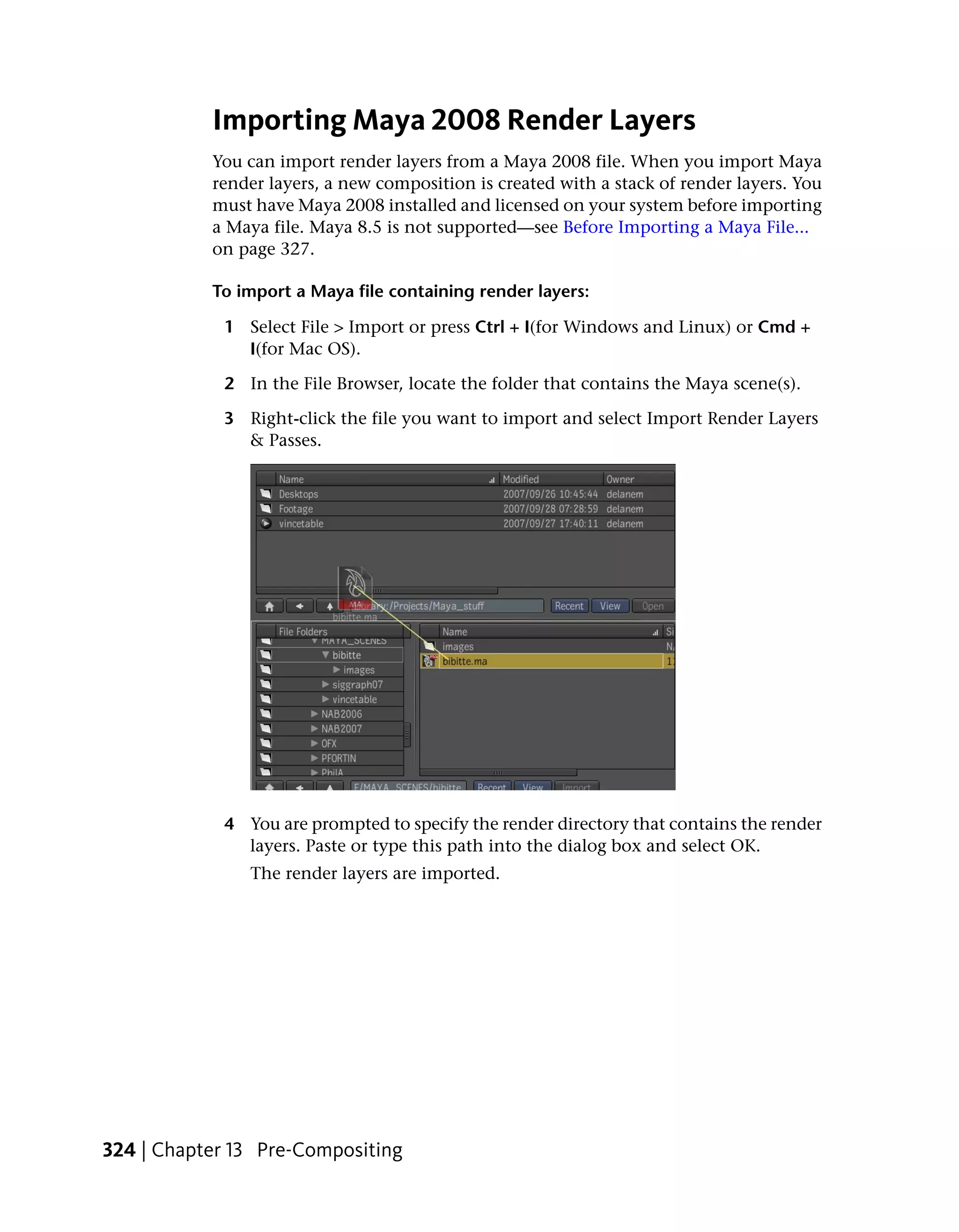
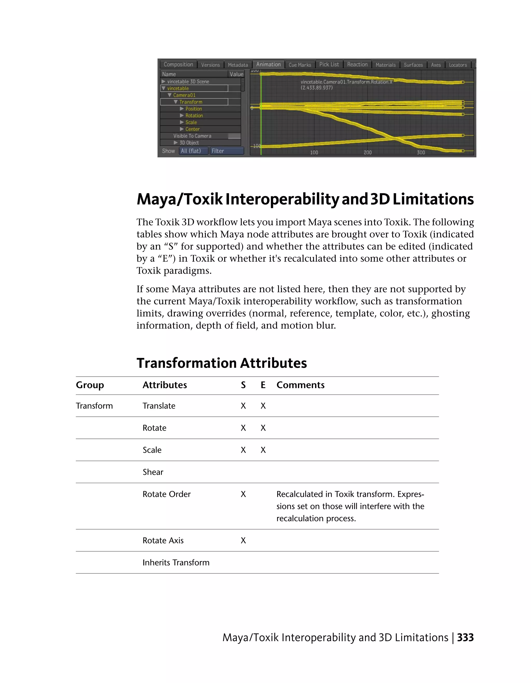
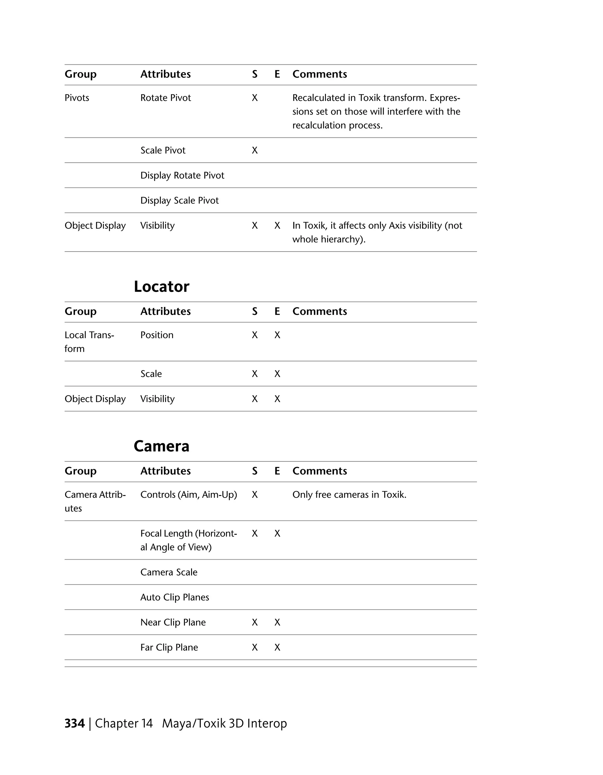
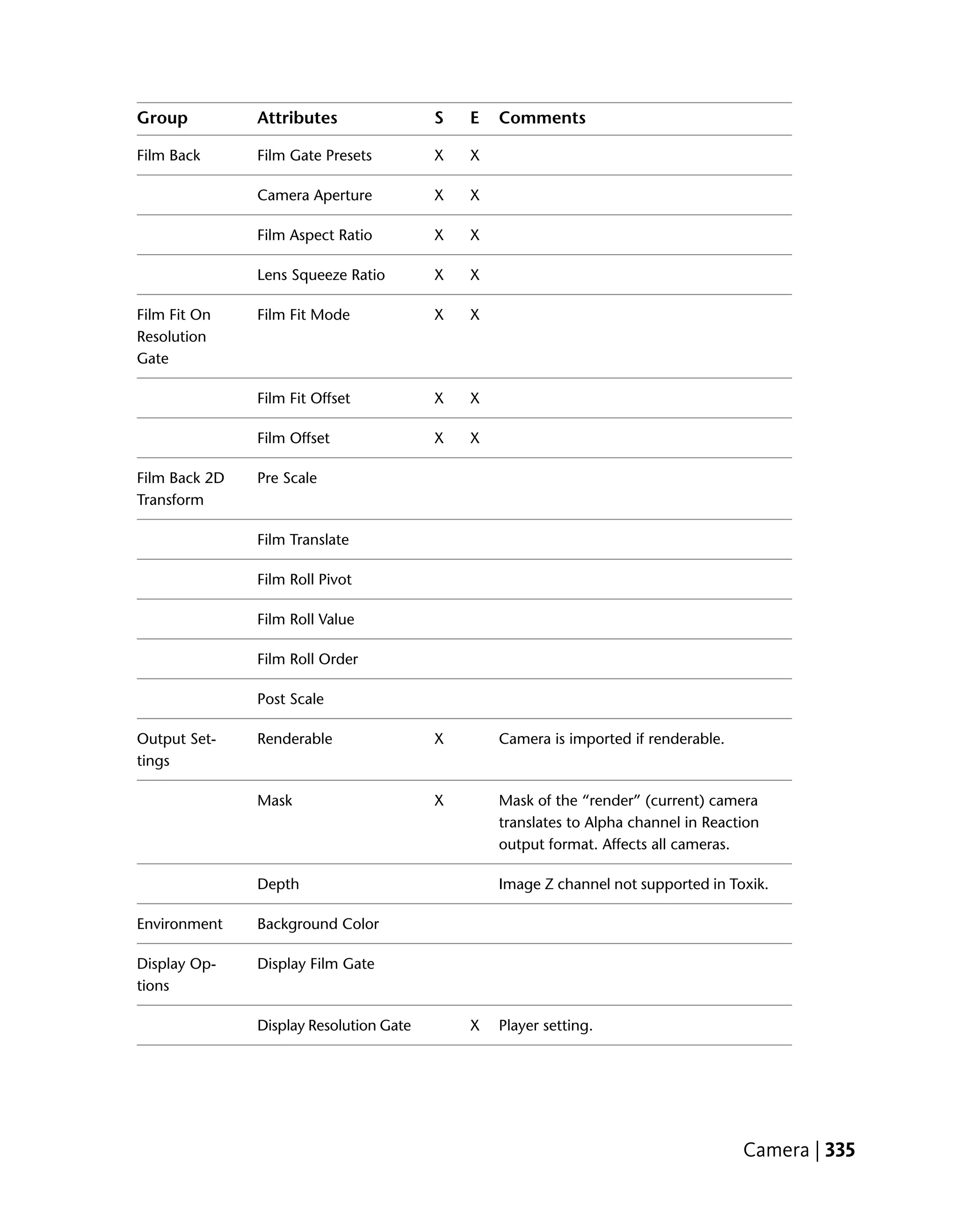
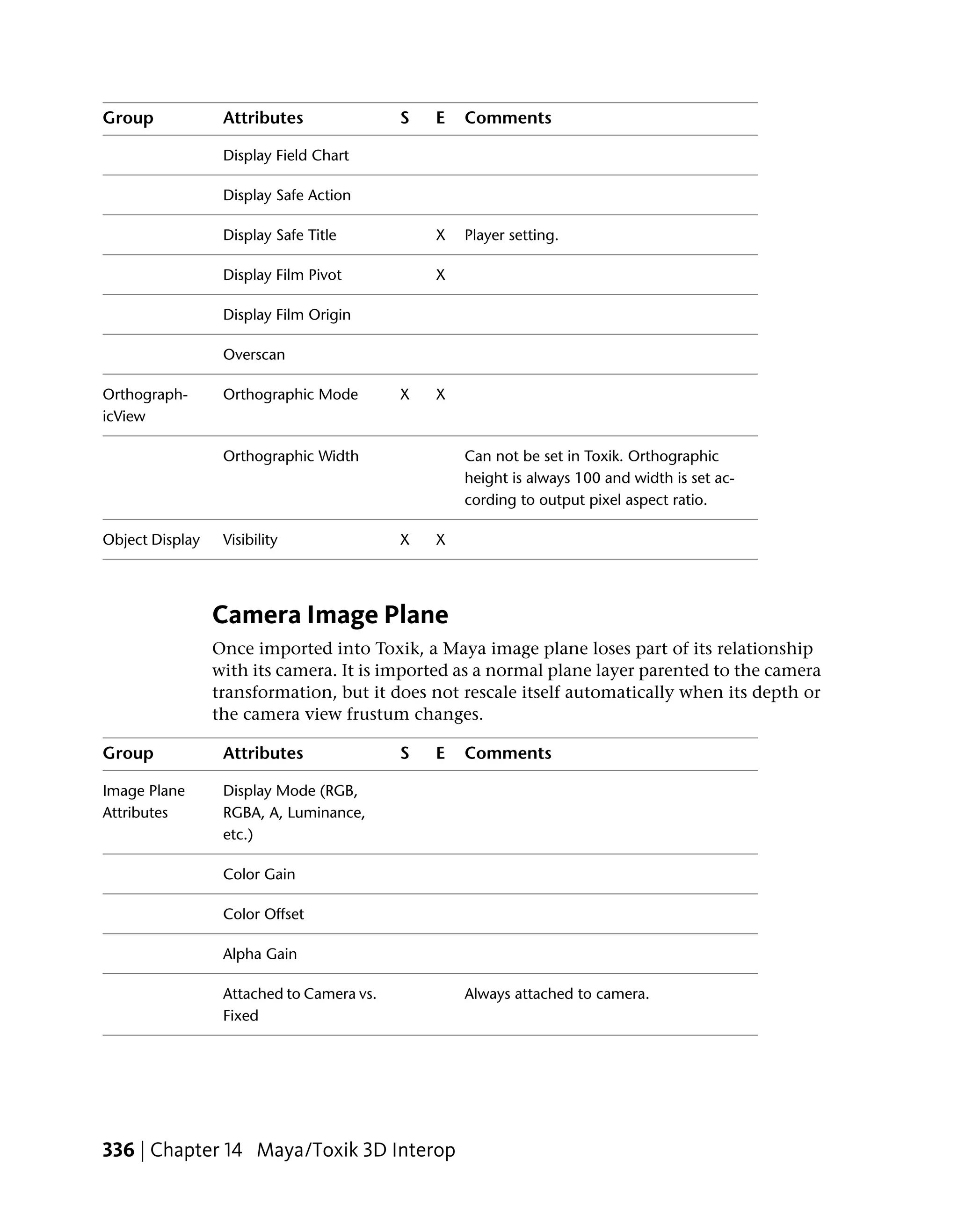
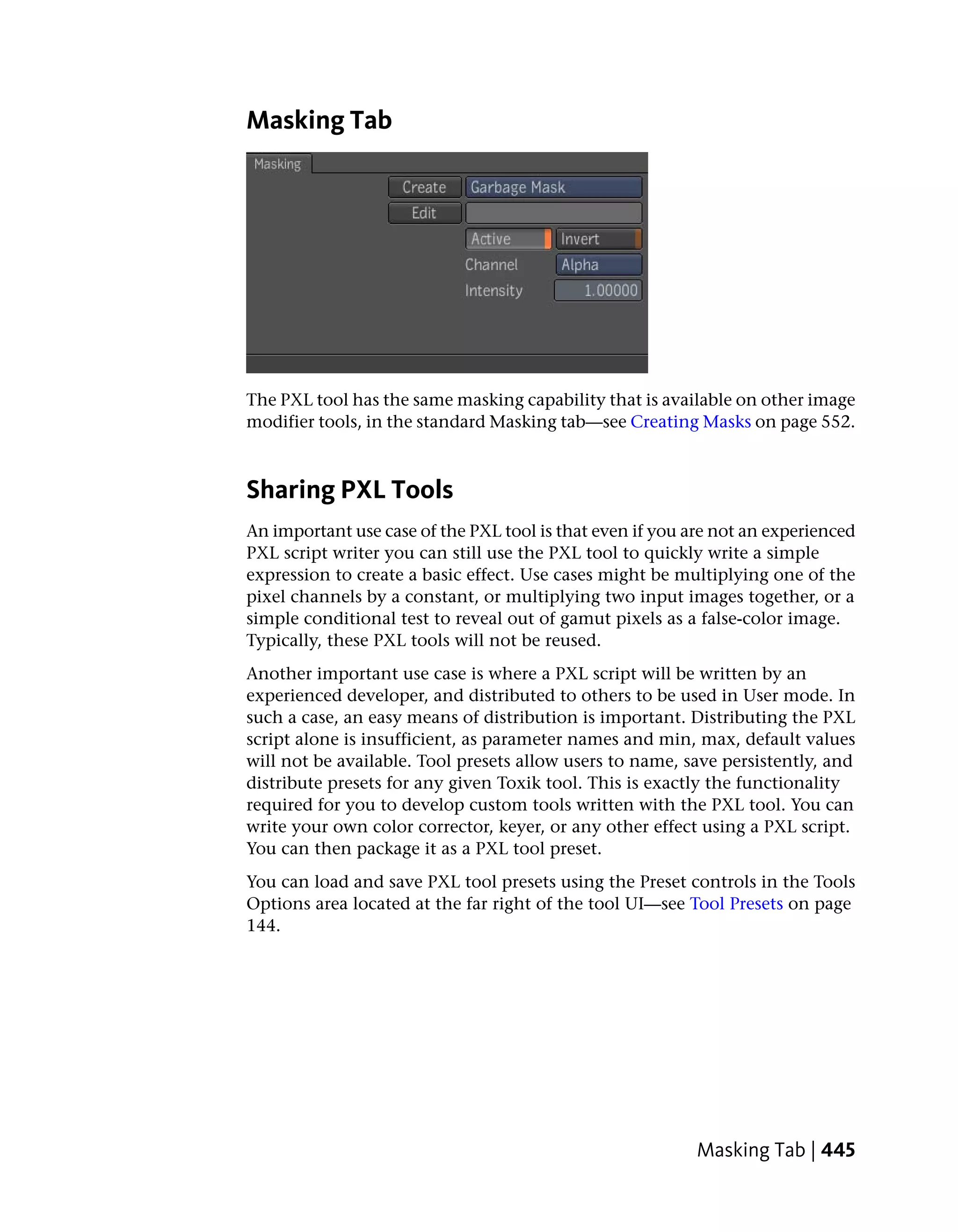
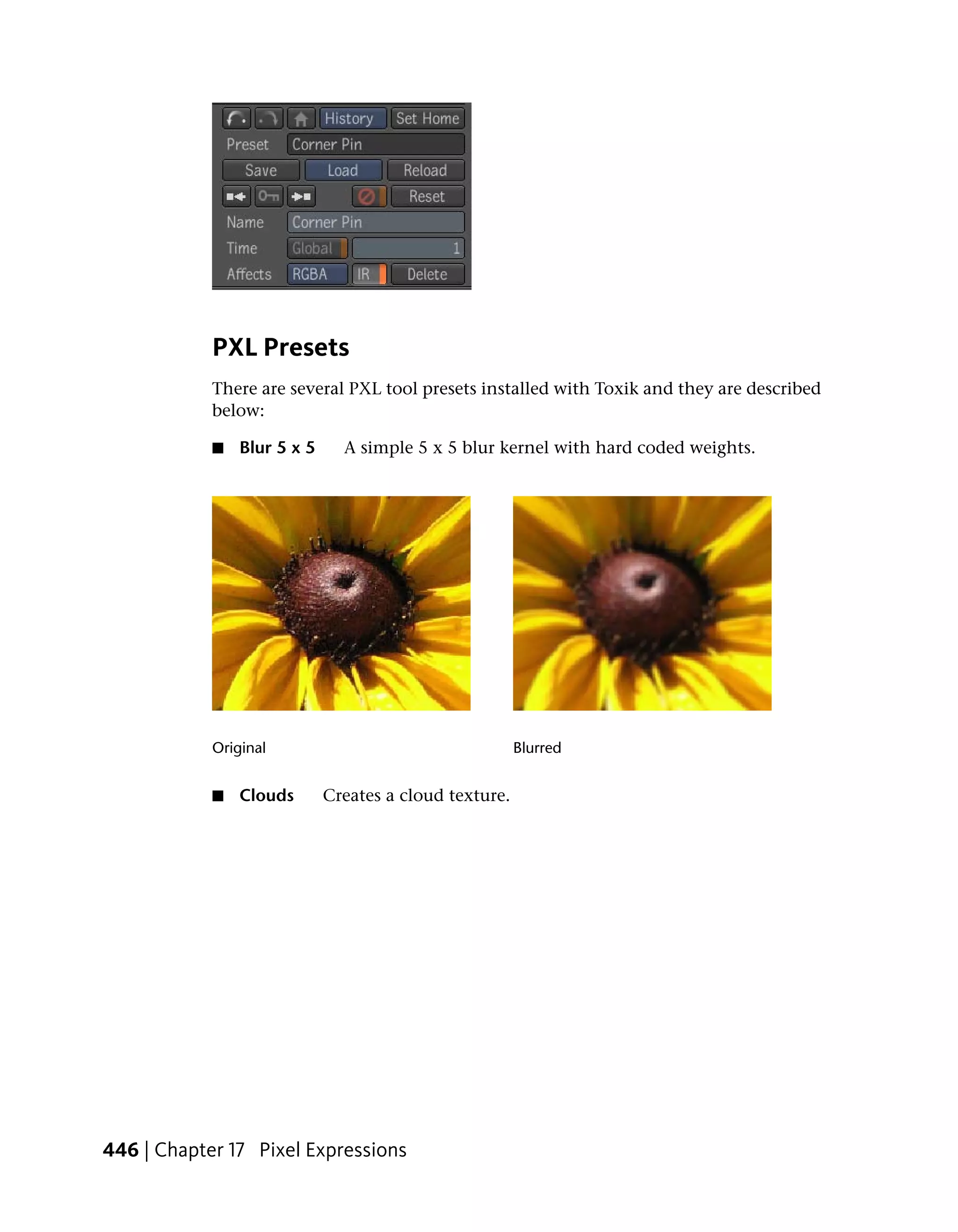
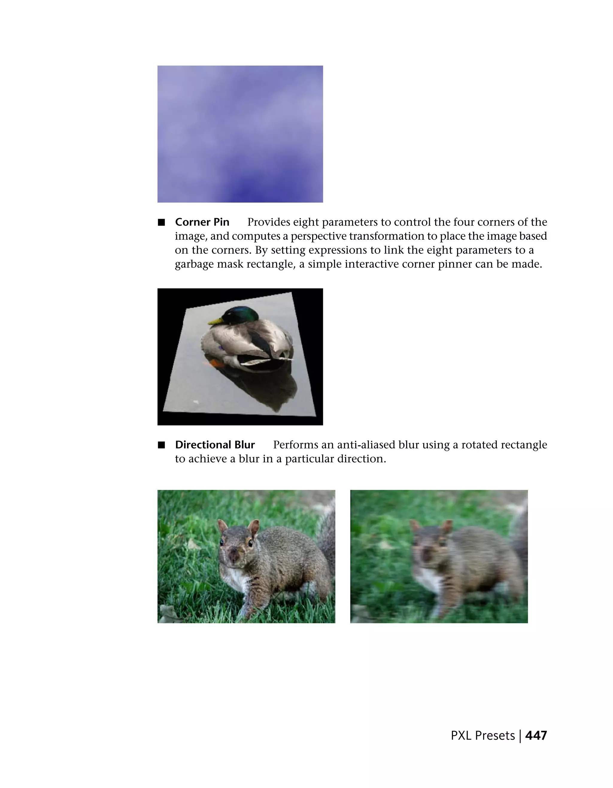
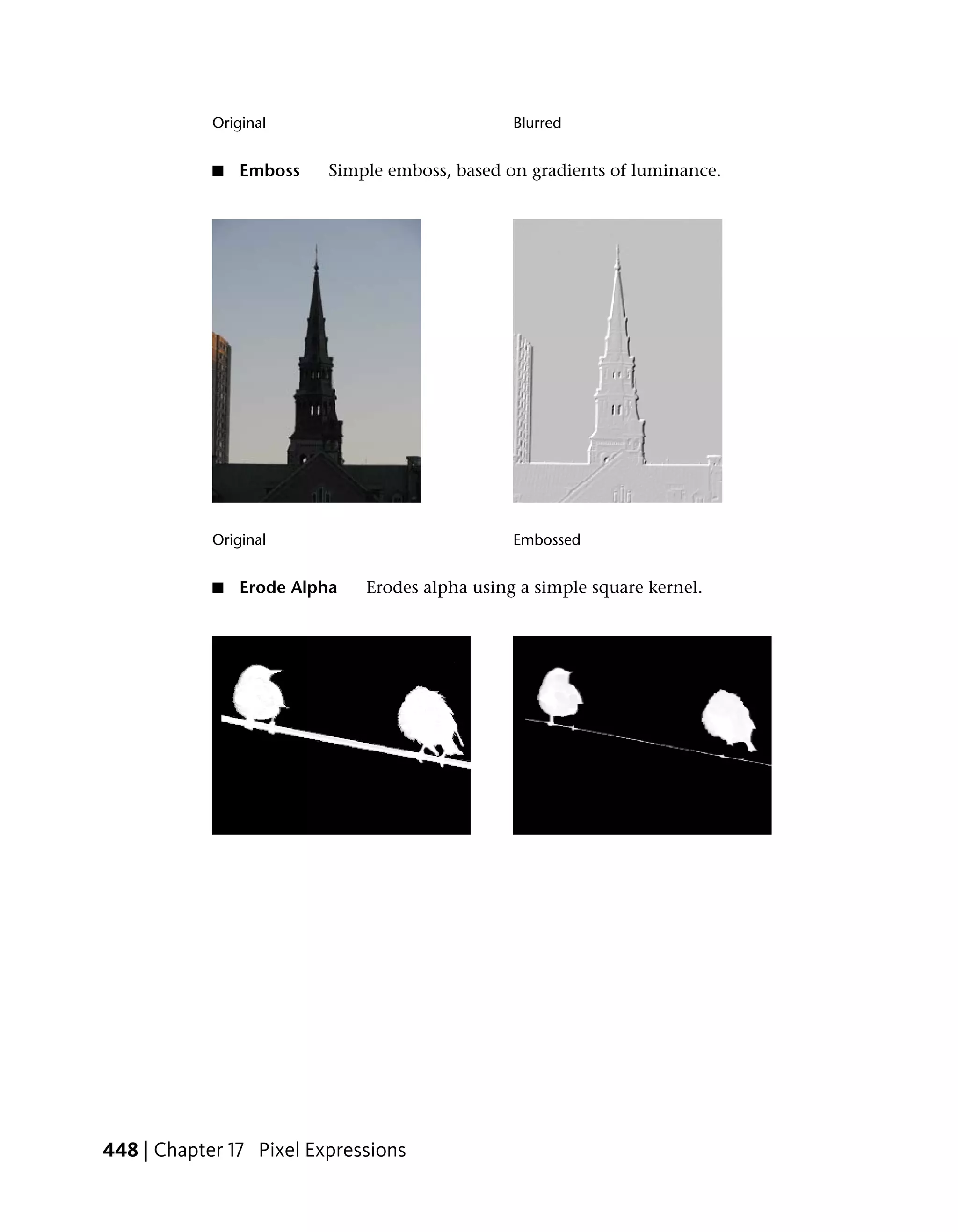
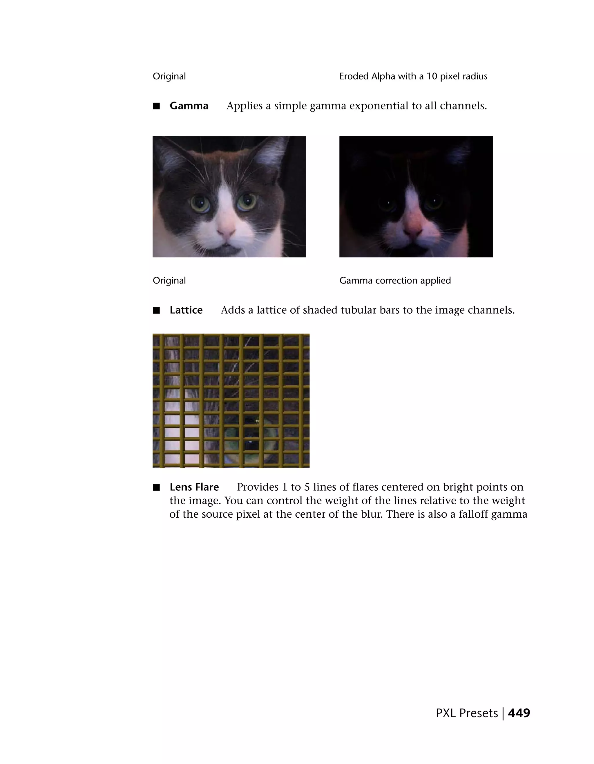
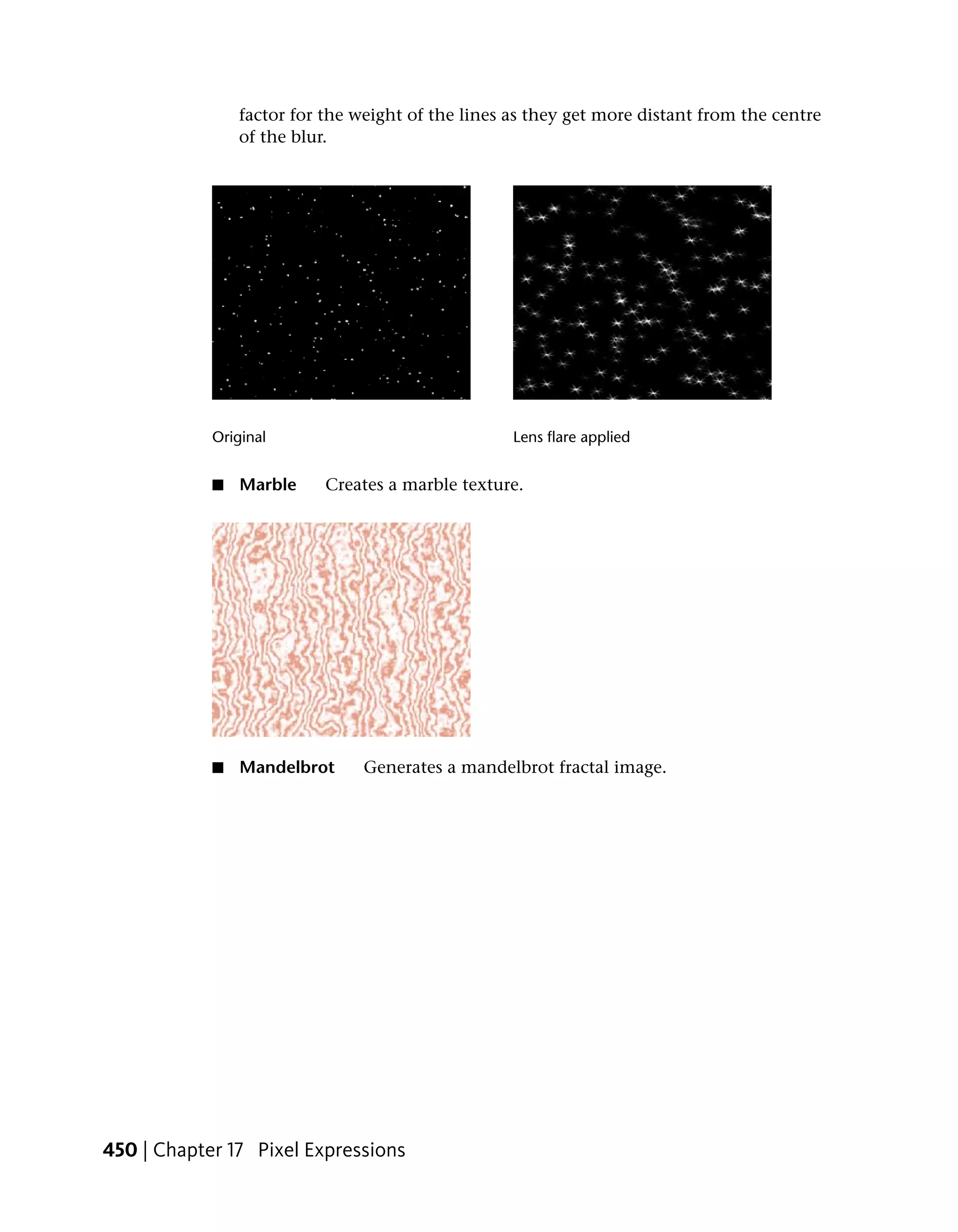
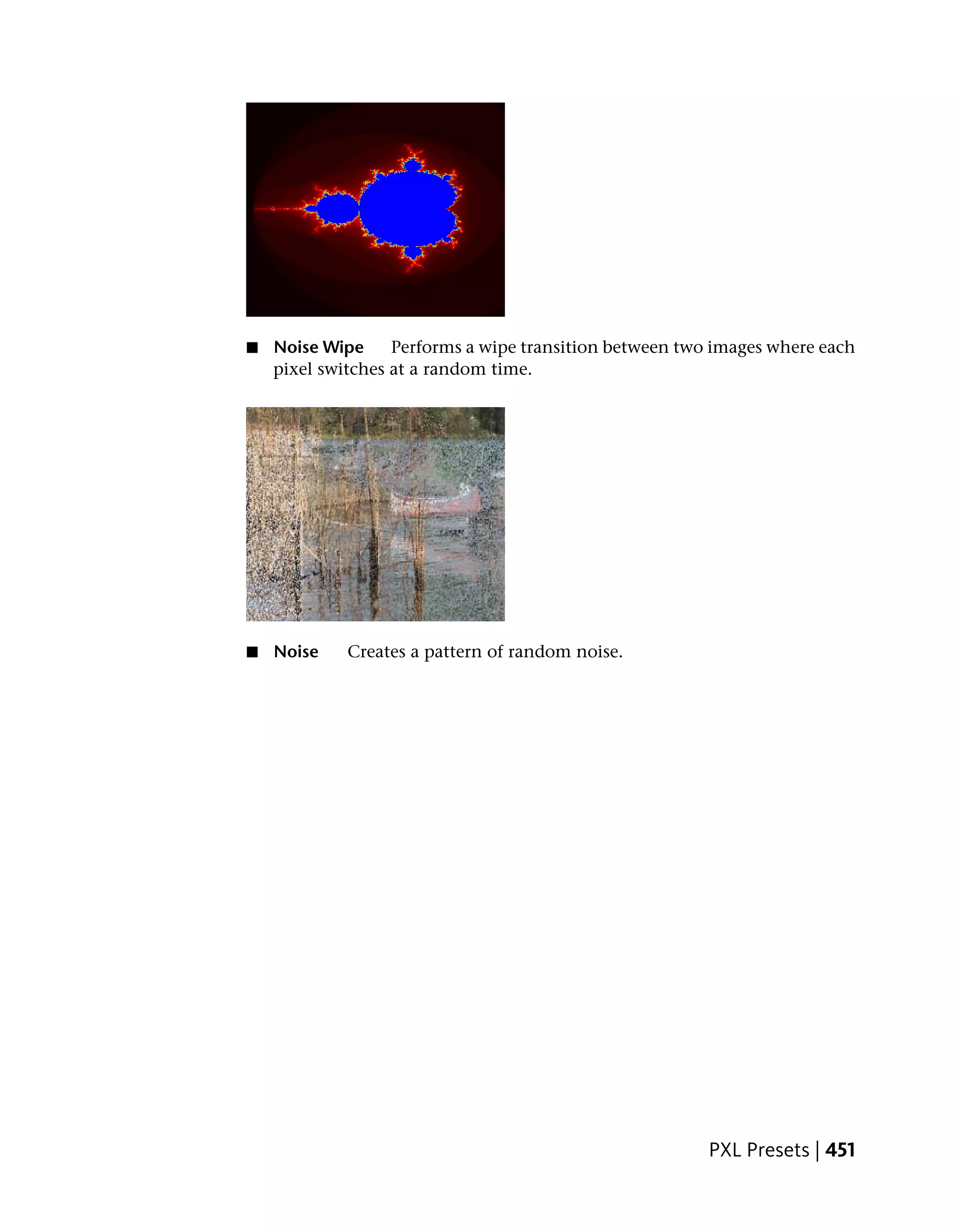
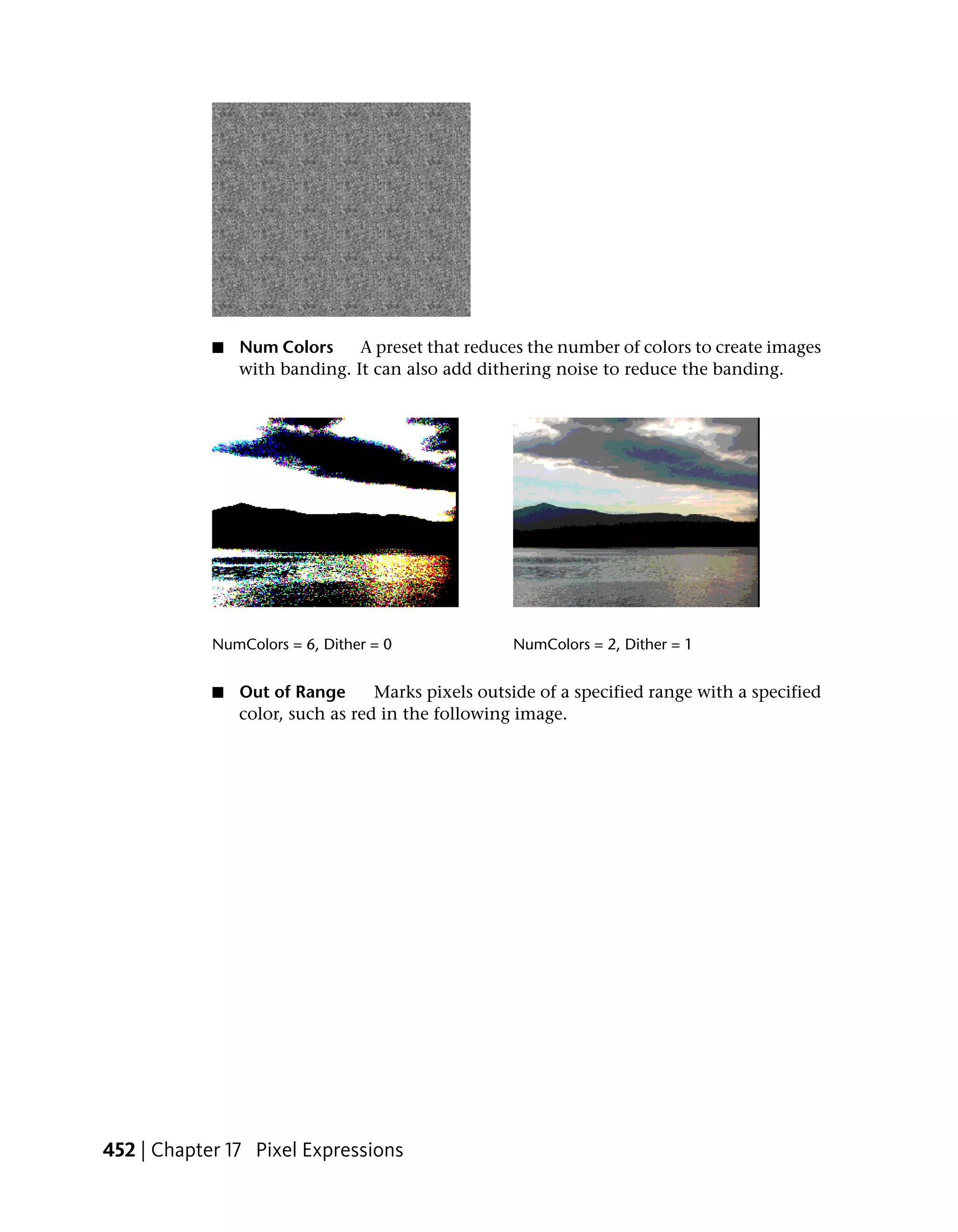
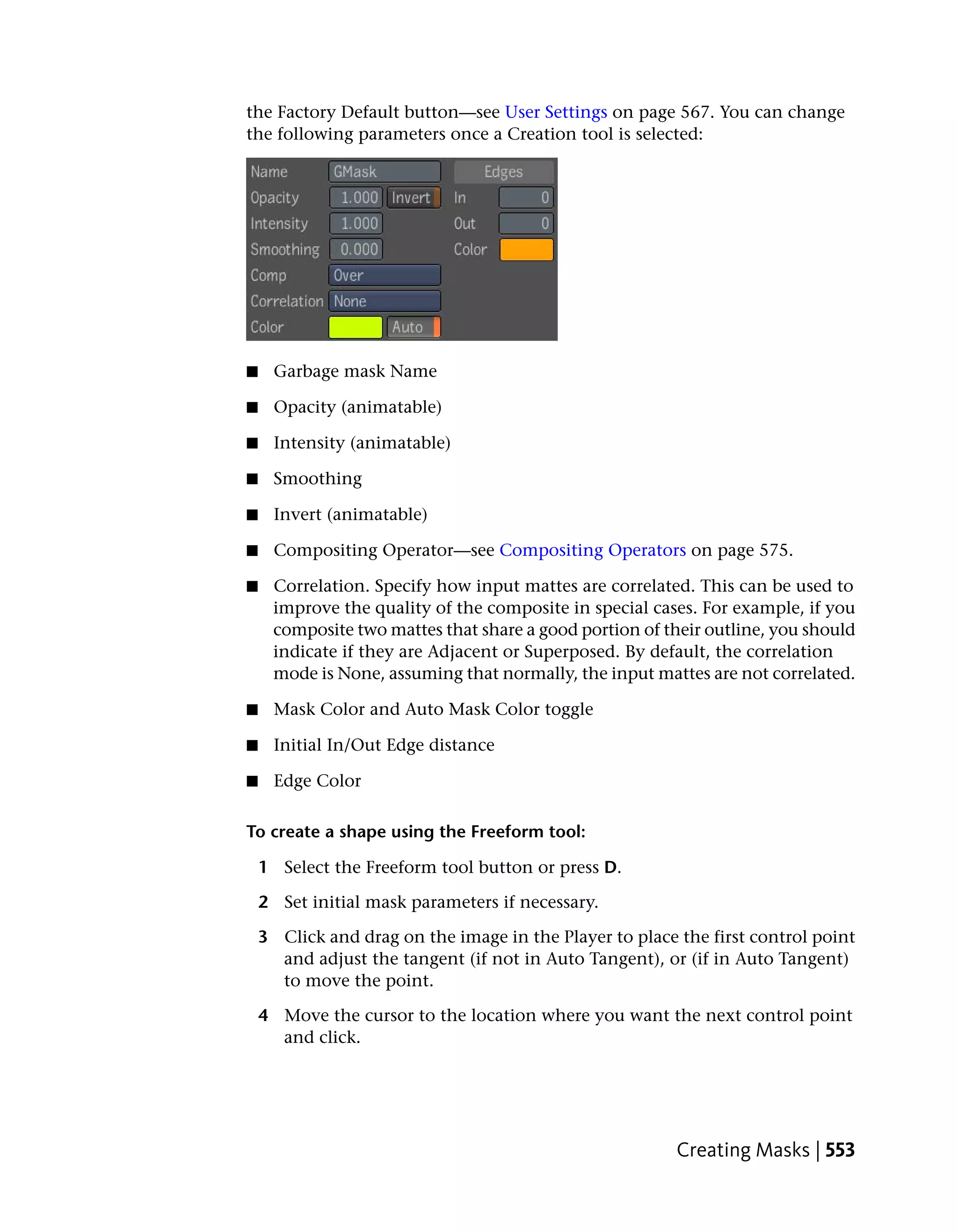
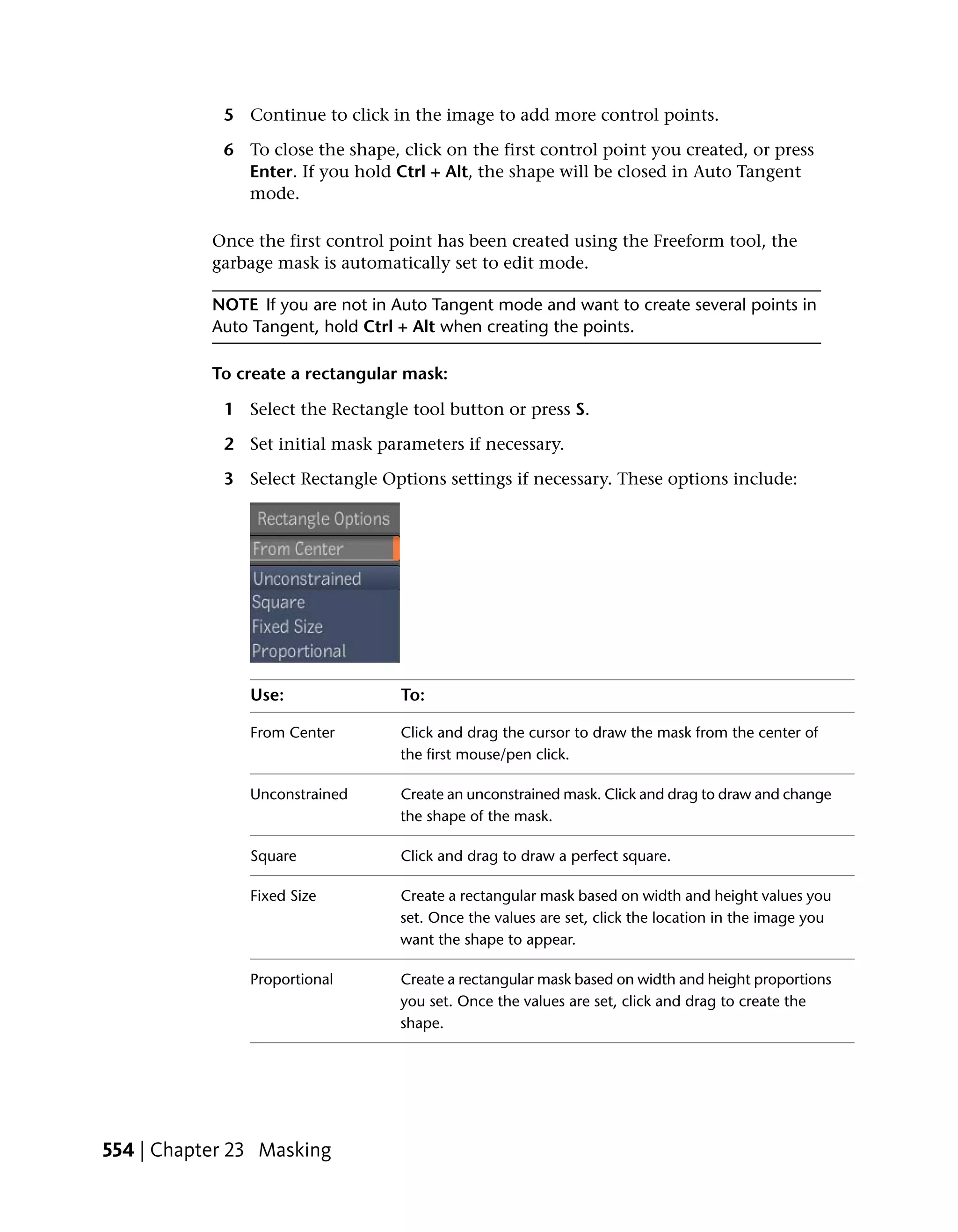
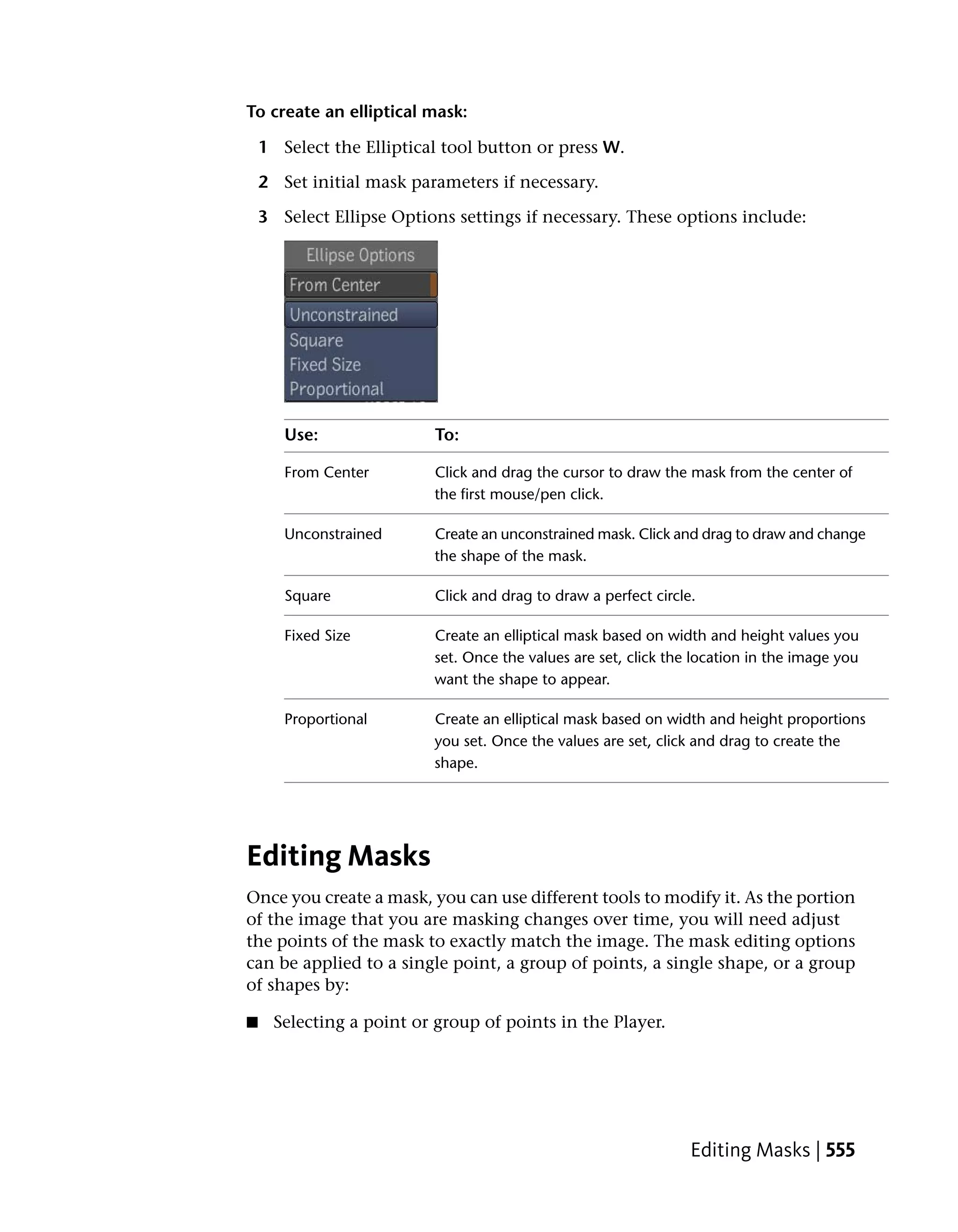
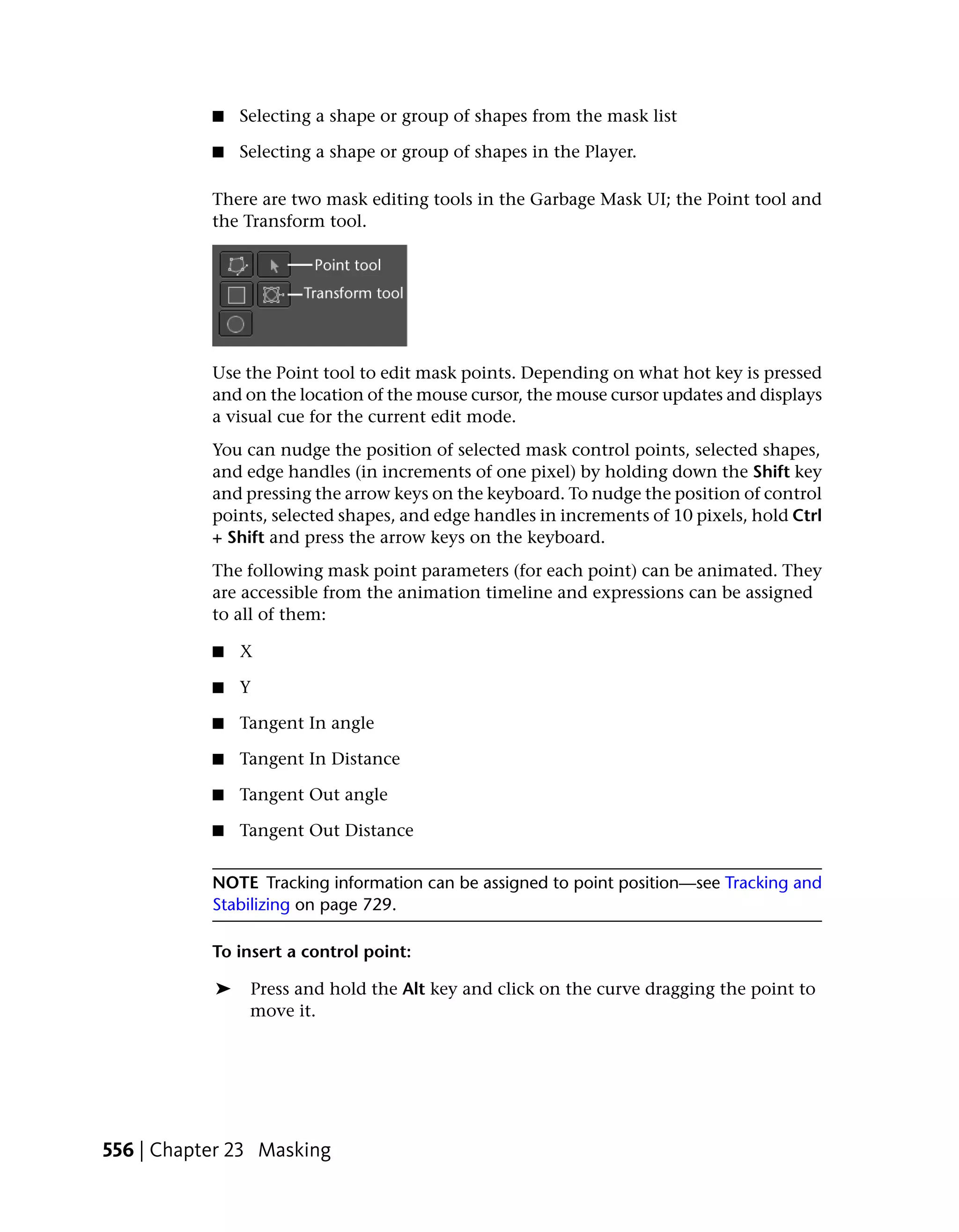
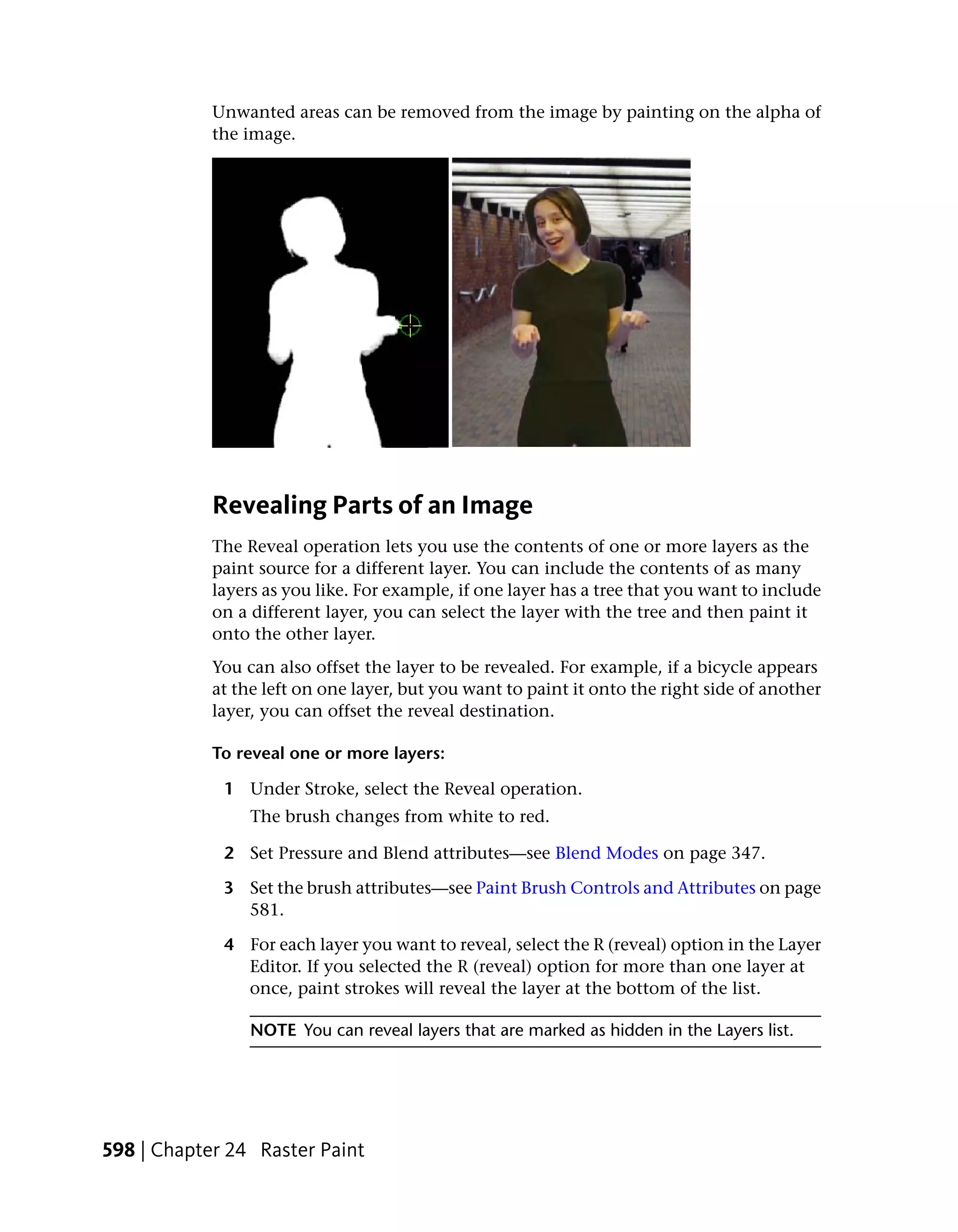
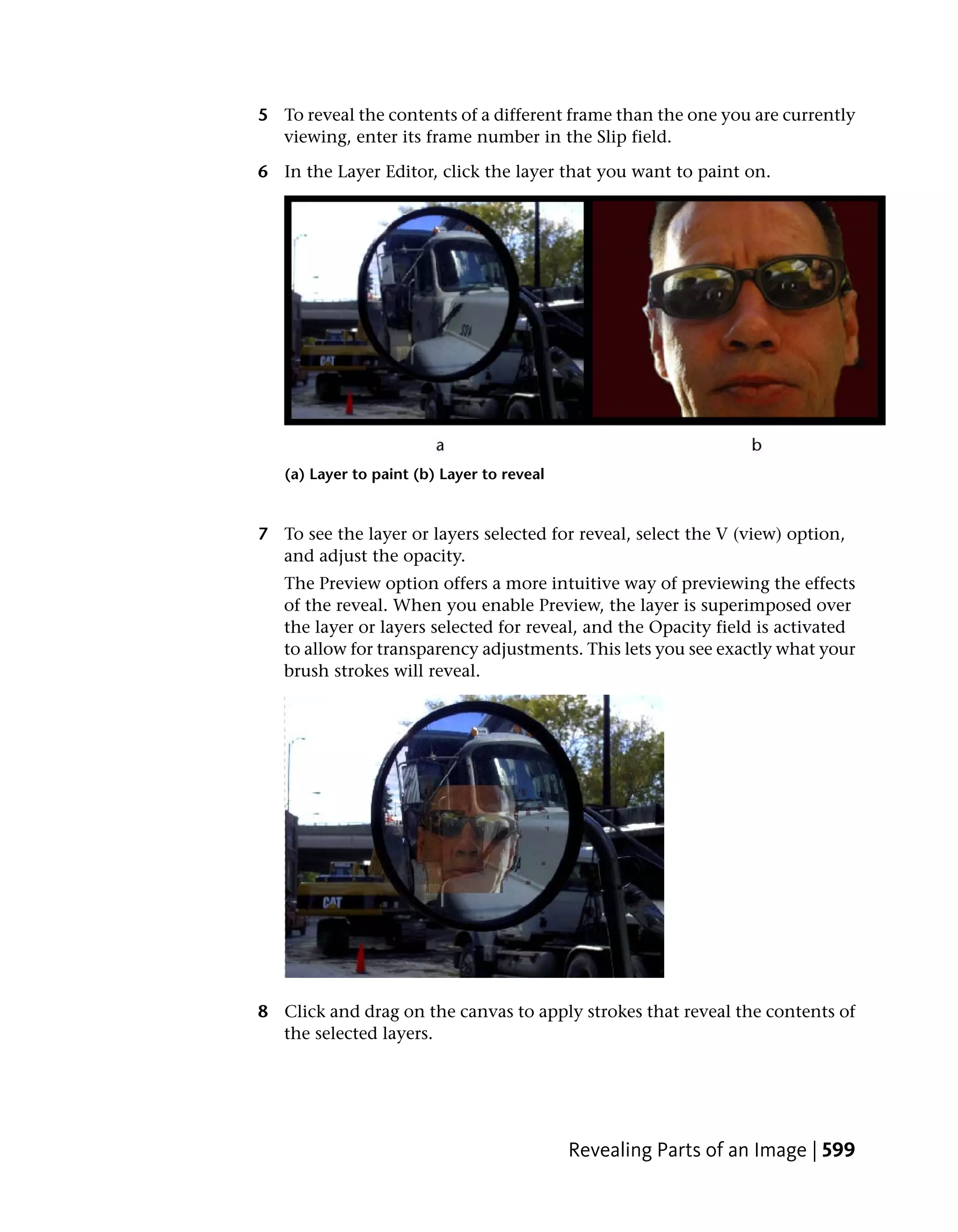
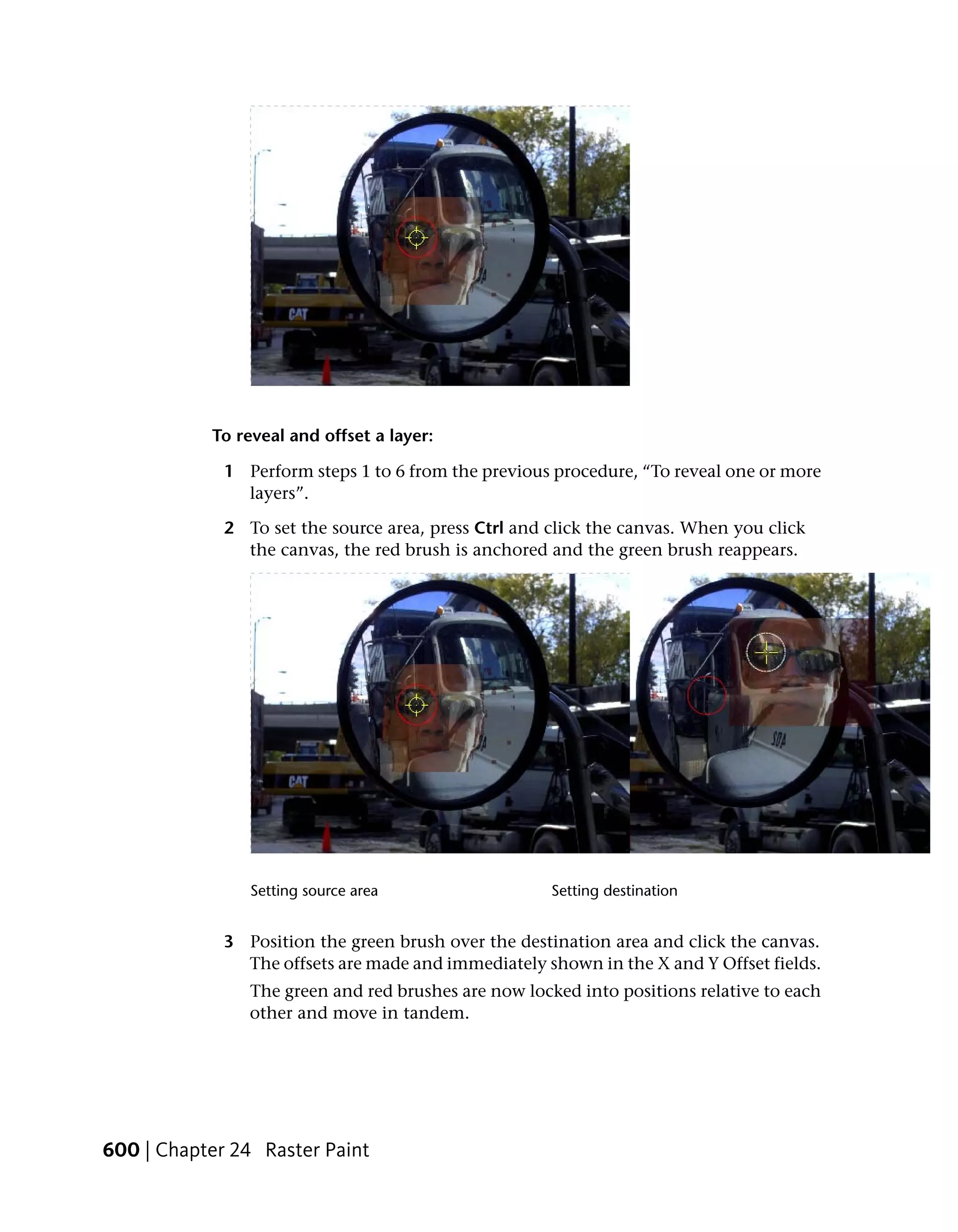
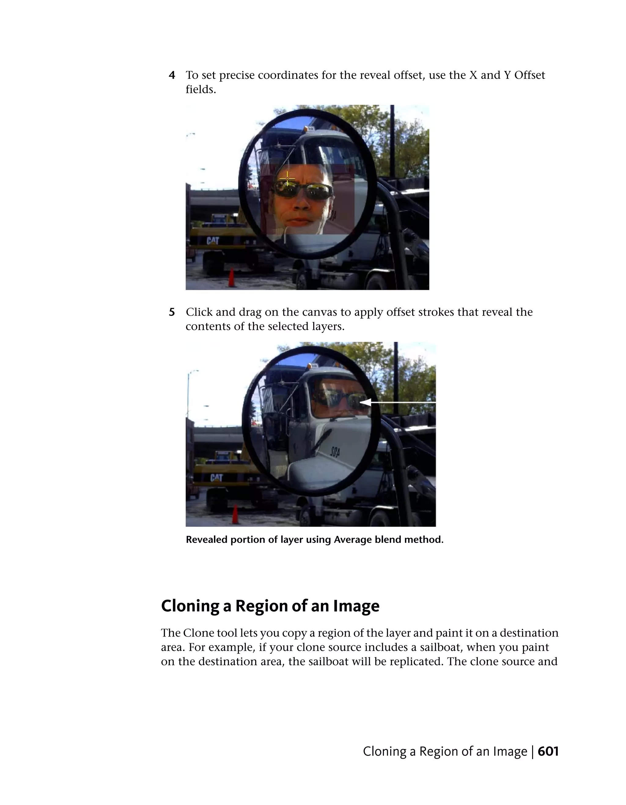
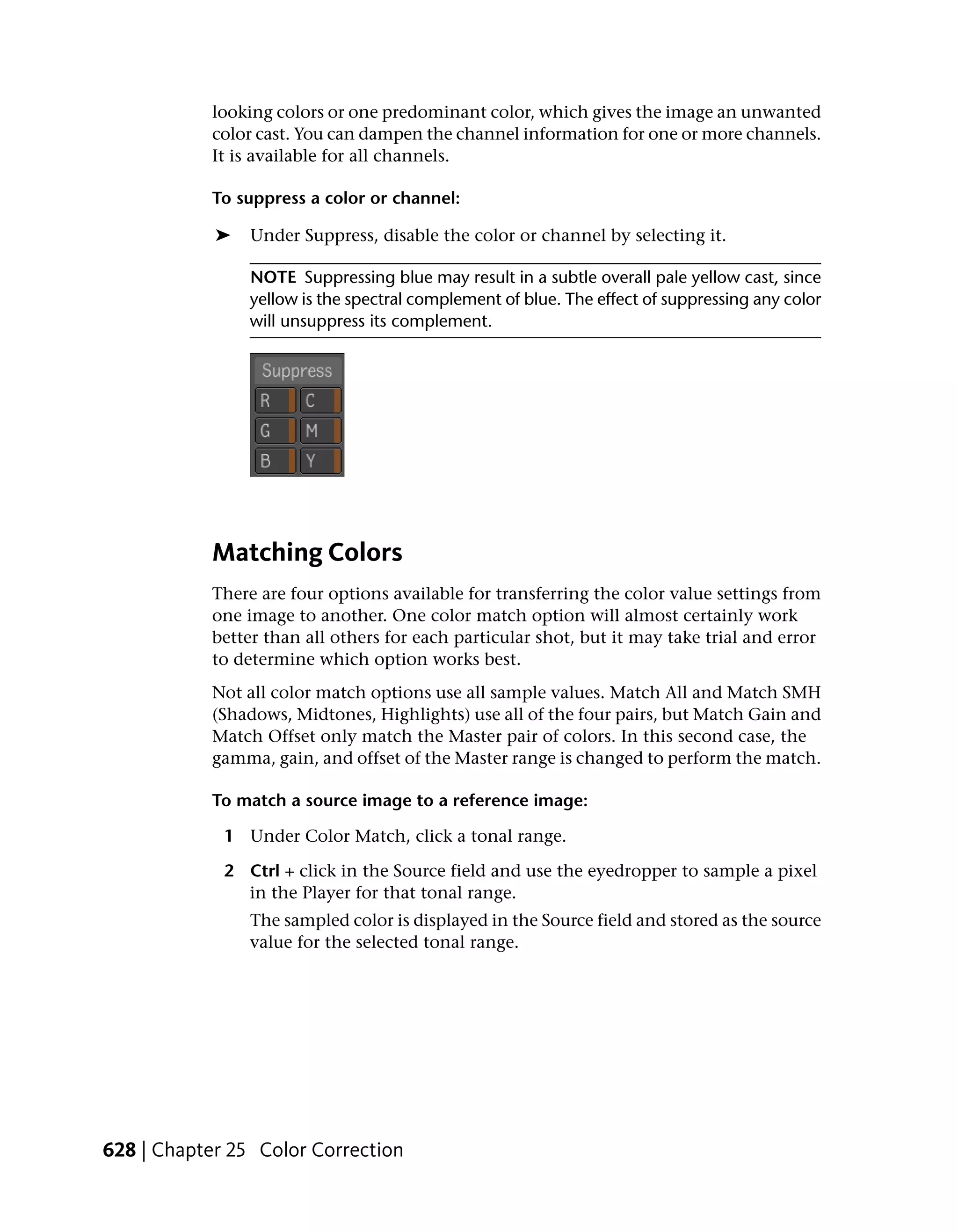
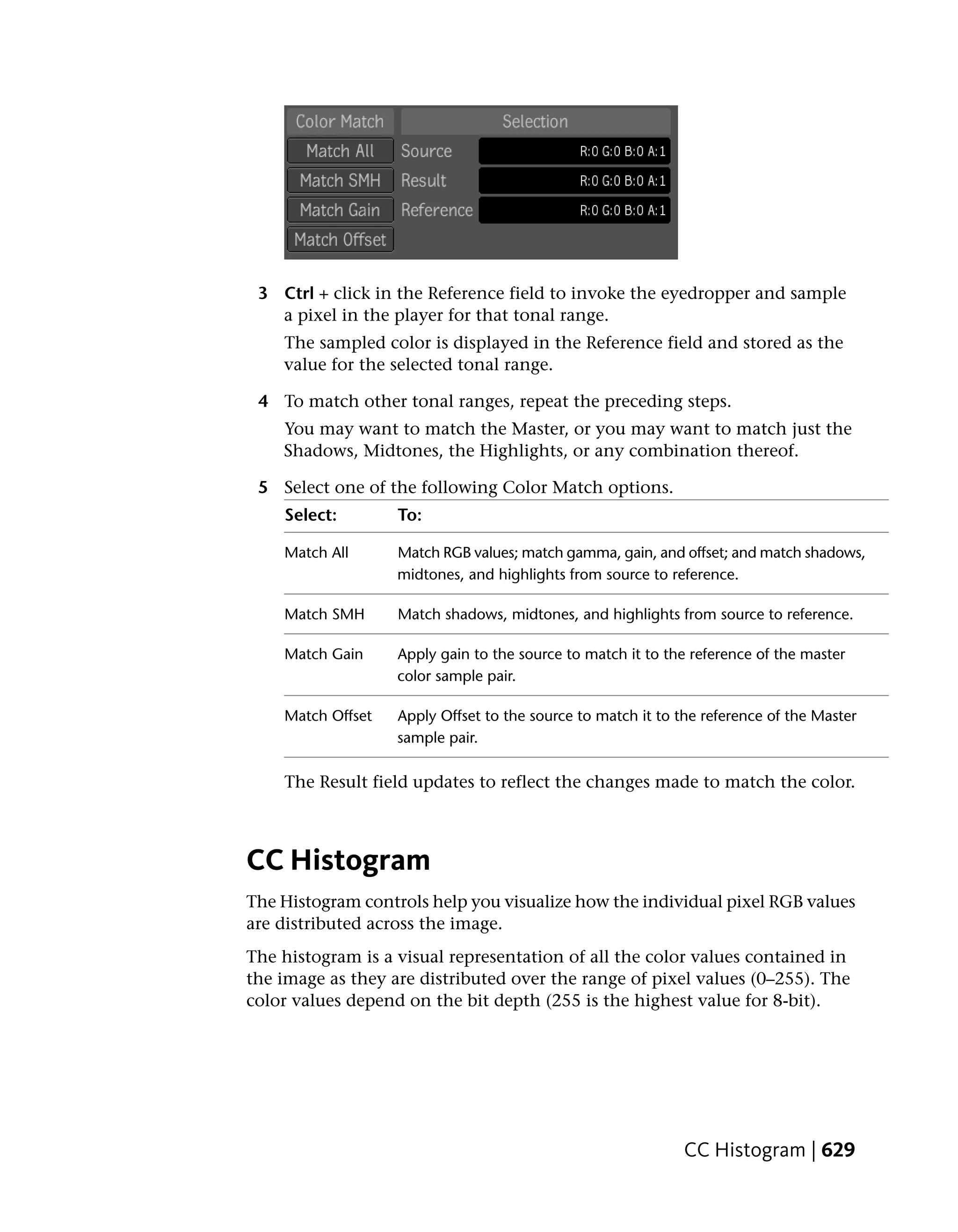
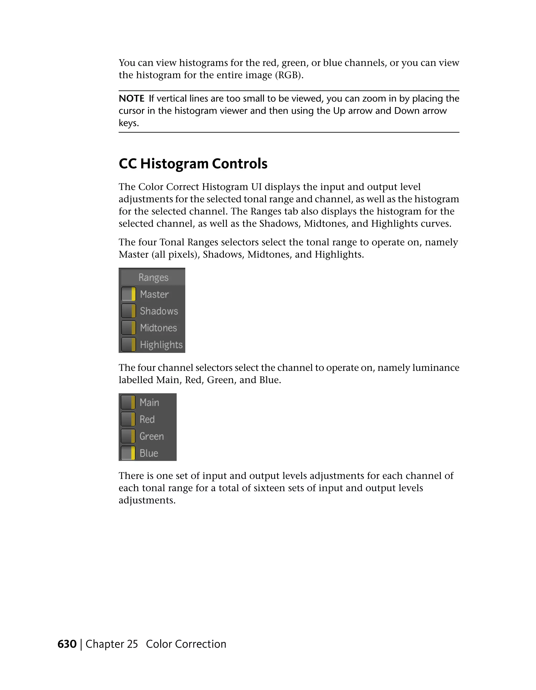
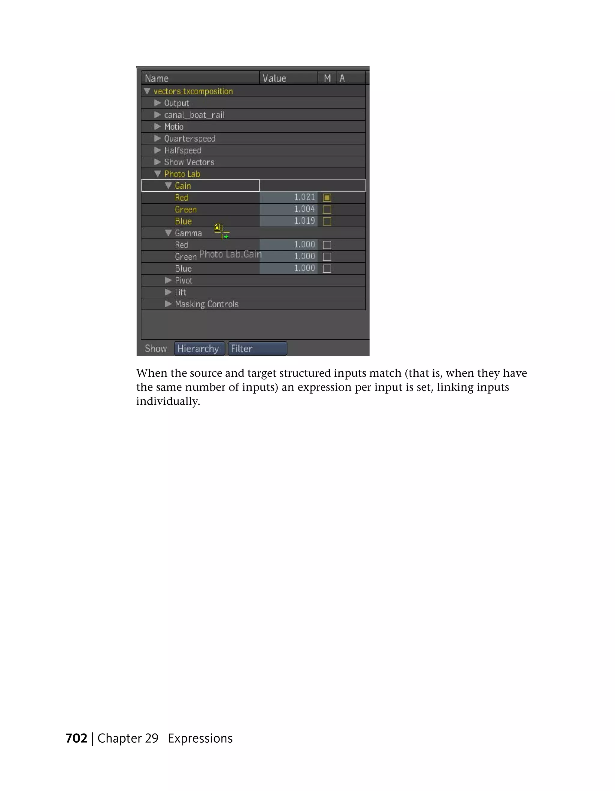
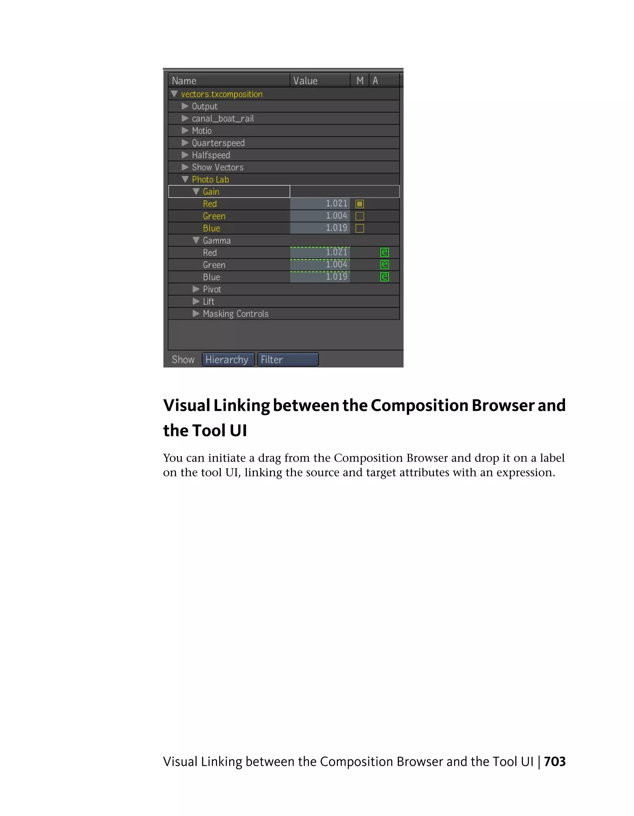
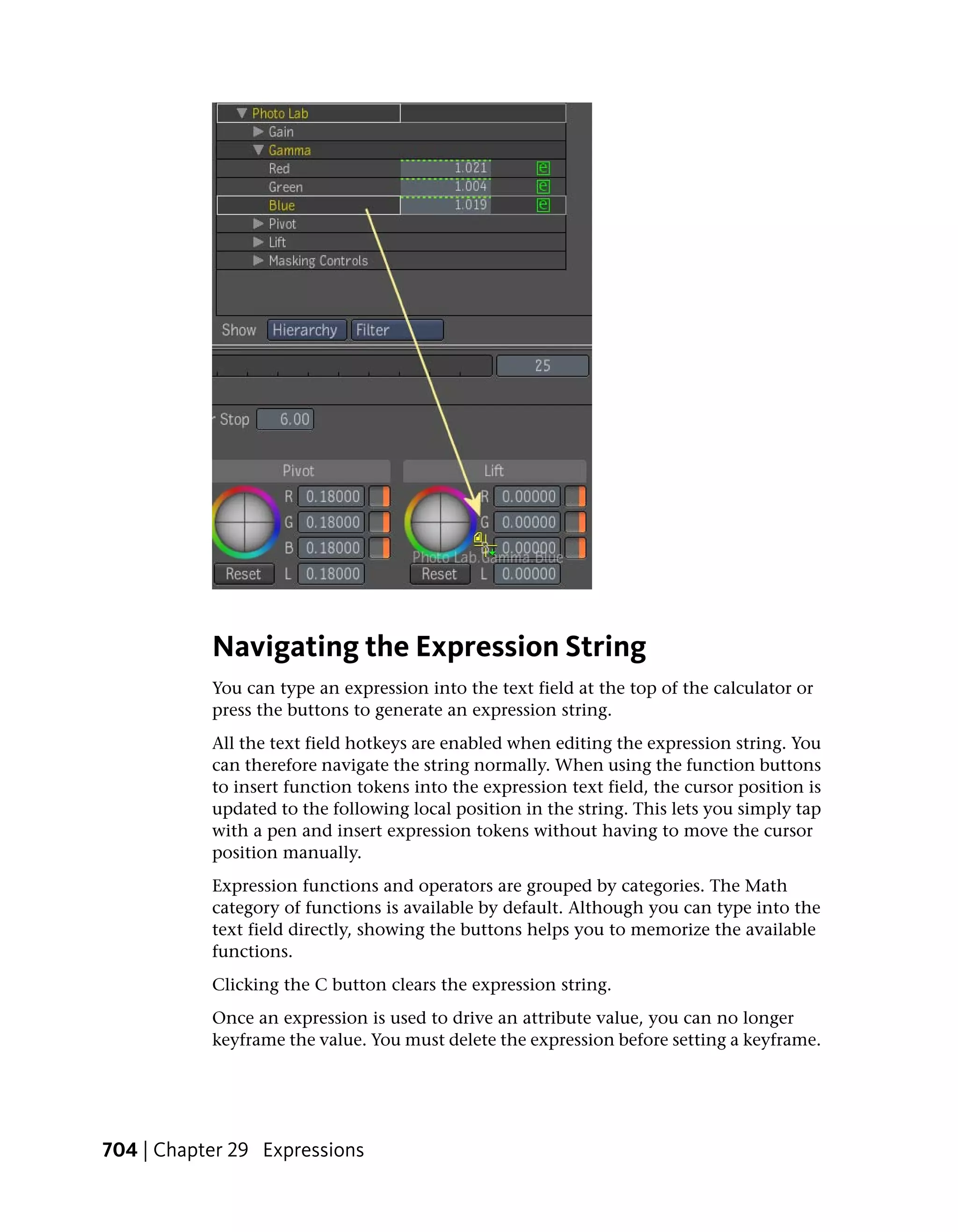
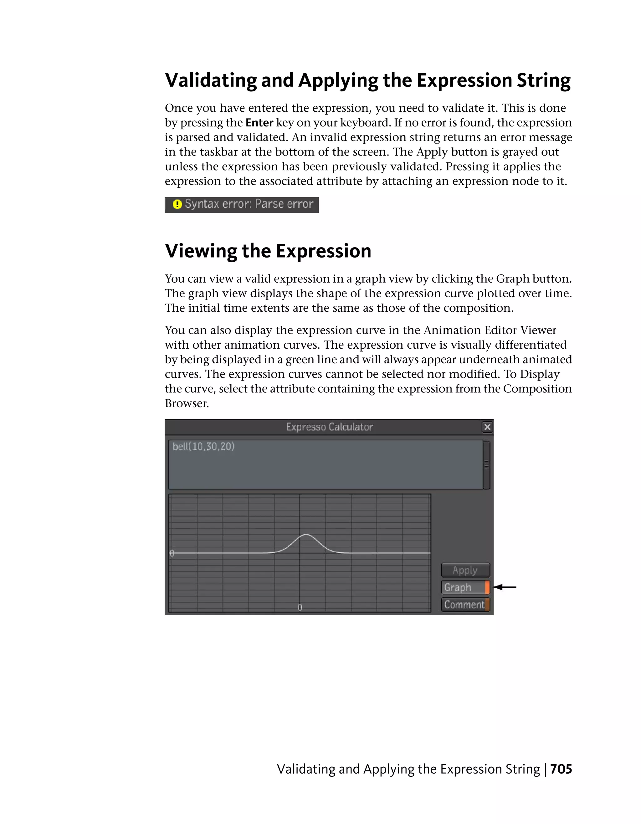
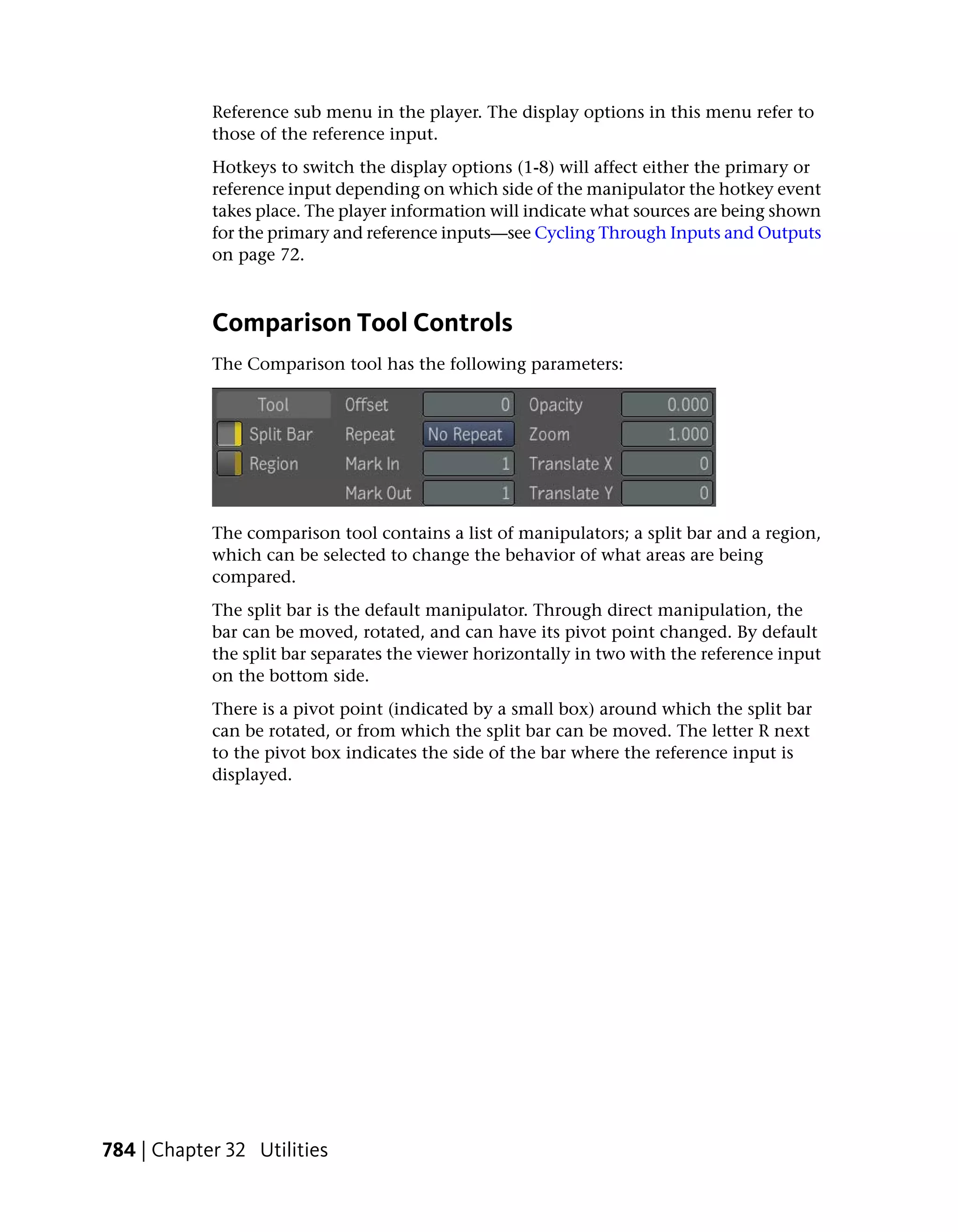
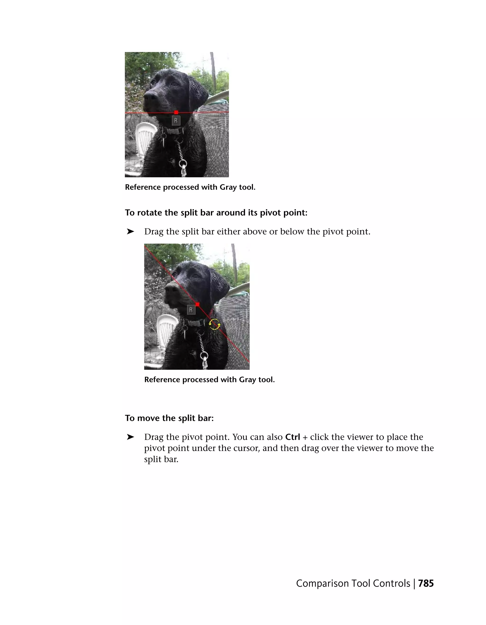
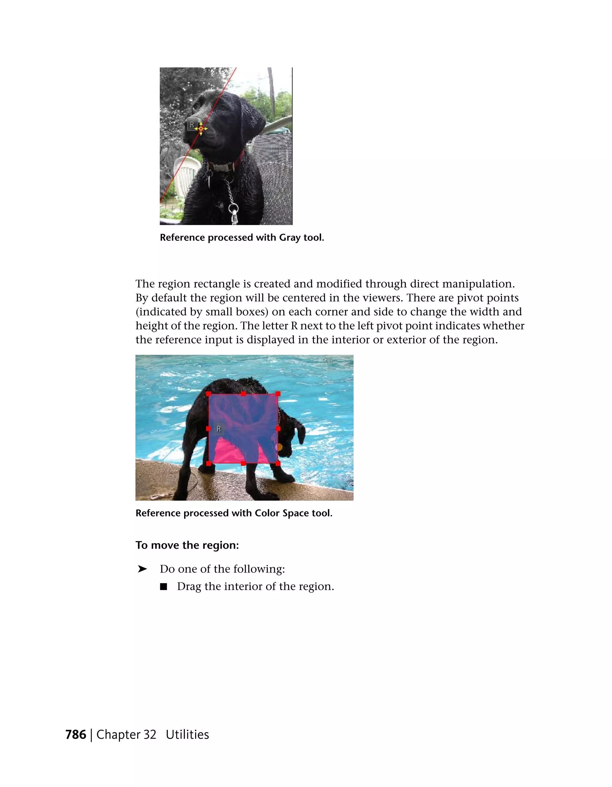
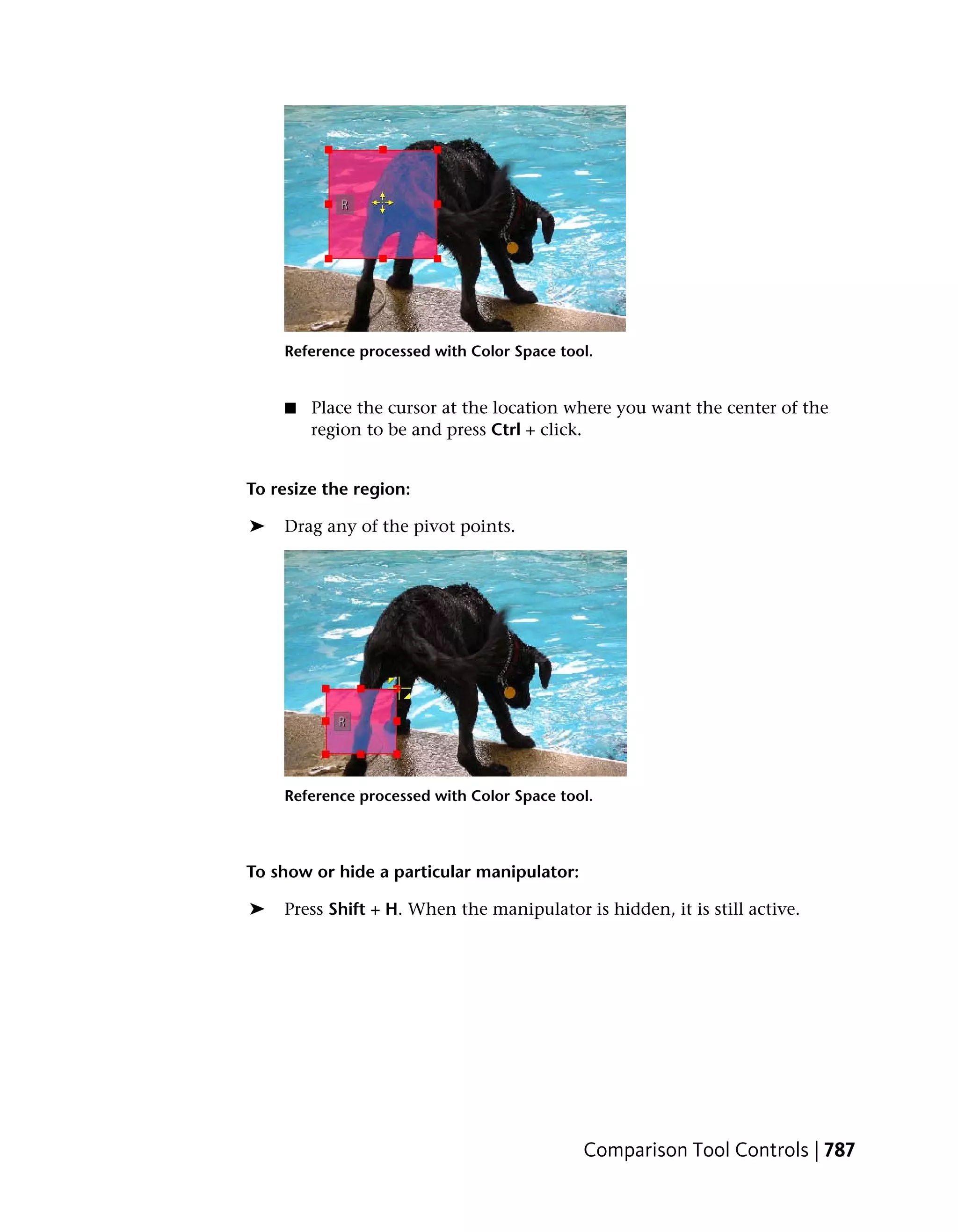
The document is the user's guide for Autodesk's Toxik software. It lists various third-party software credits and attributions, acknowledging the copyrights and licenses of the different components used in Toxik. It provides credits for software related to installation, graphics, animation, modeling, and programming.


