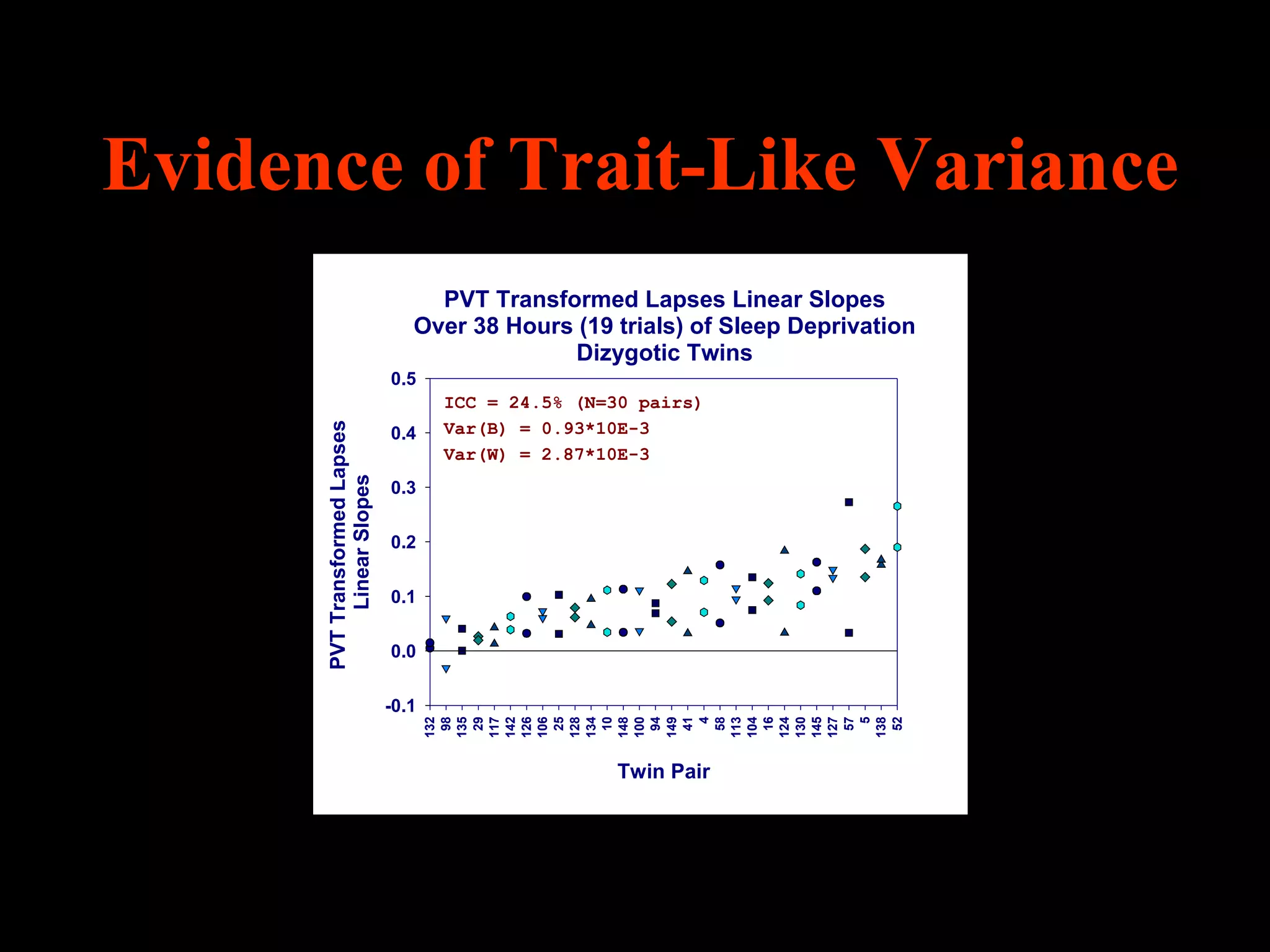
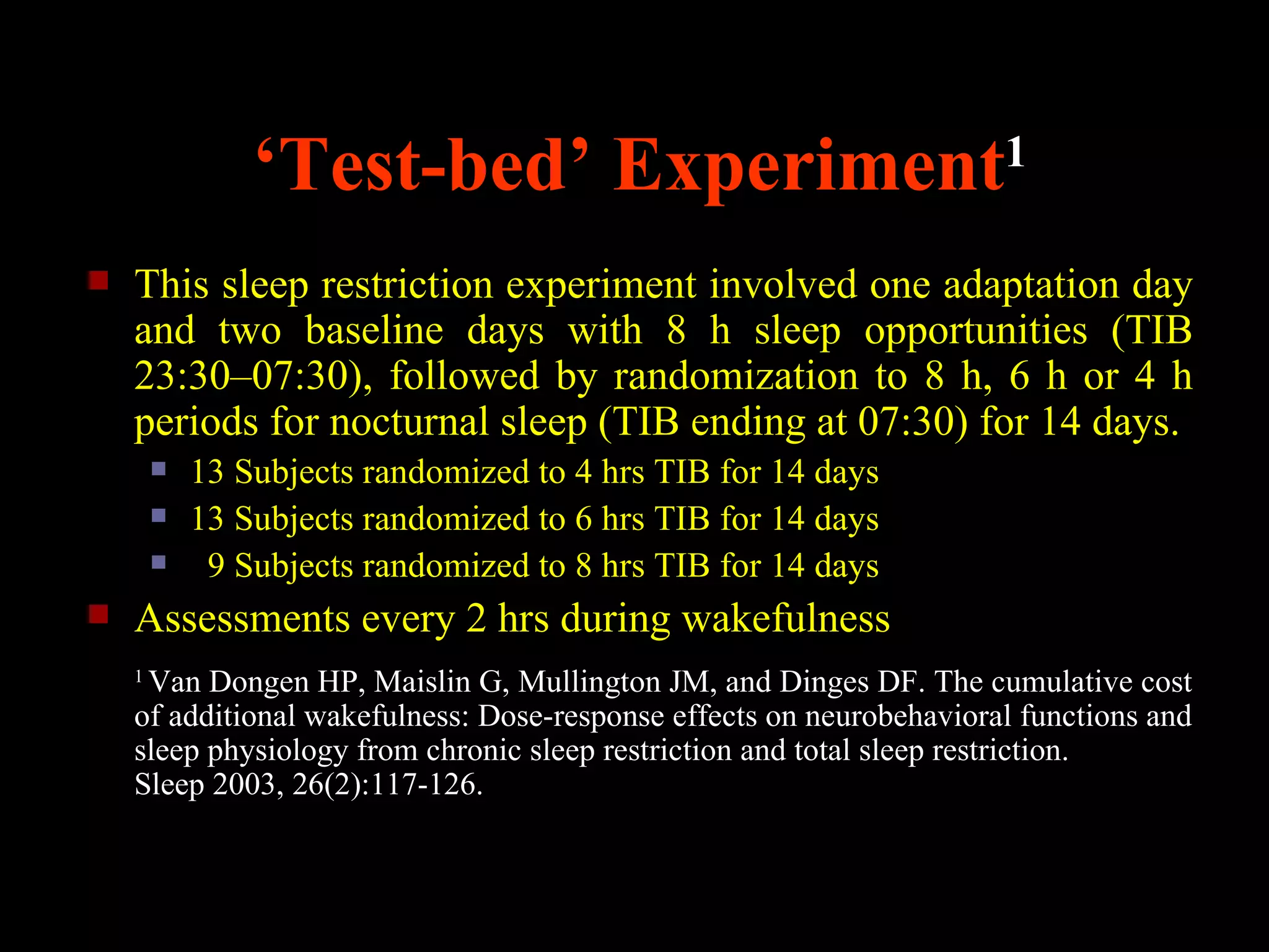
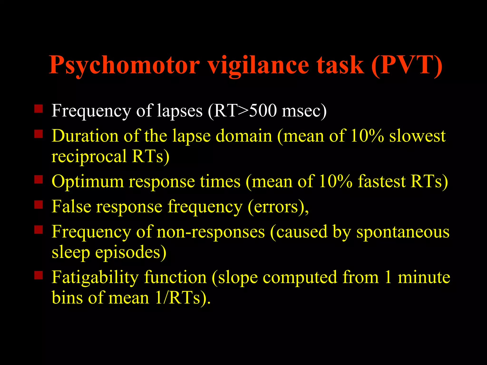
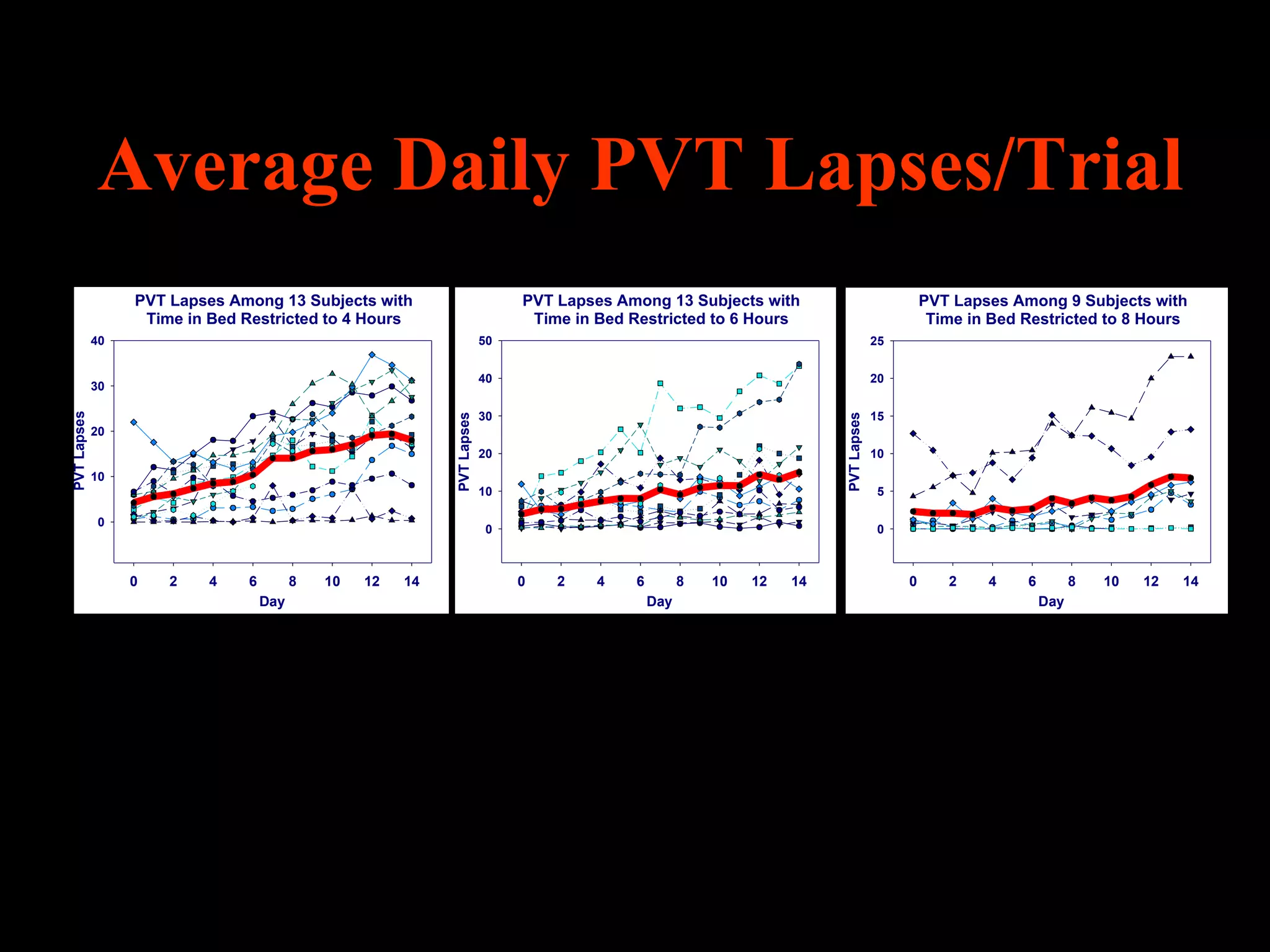
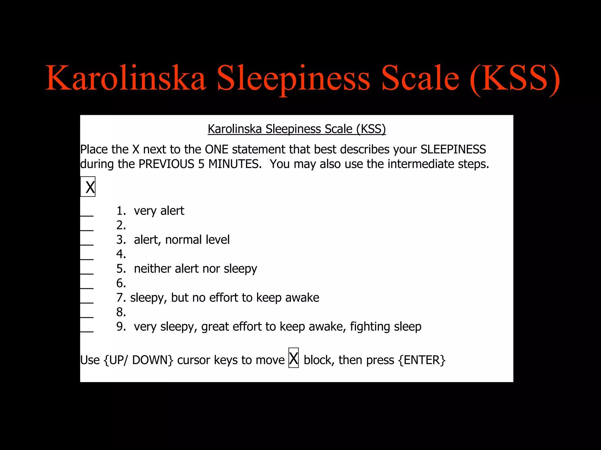
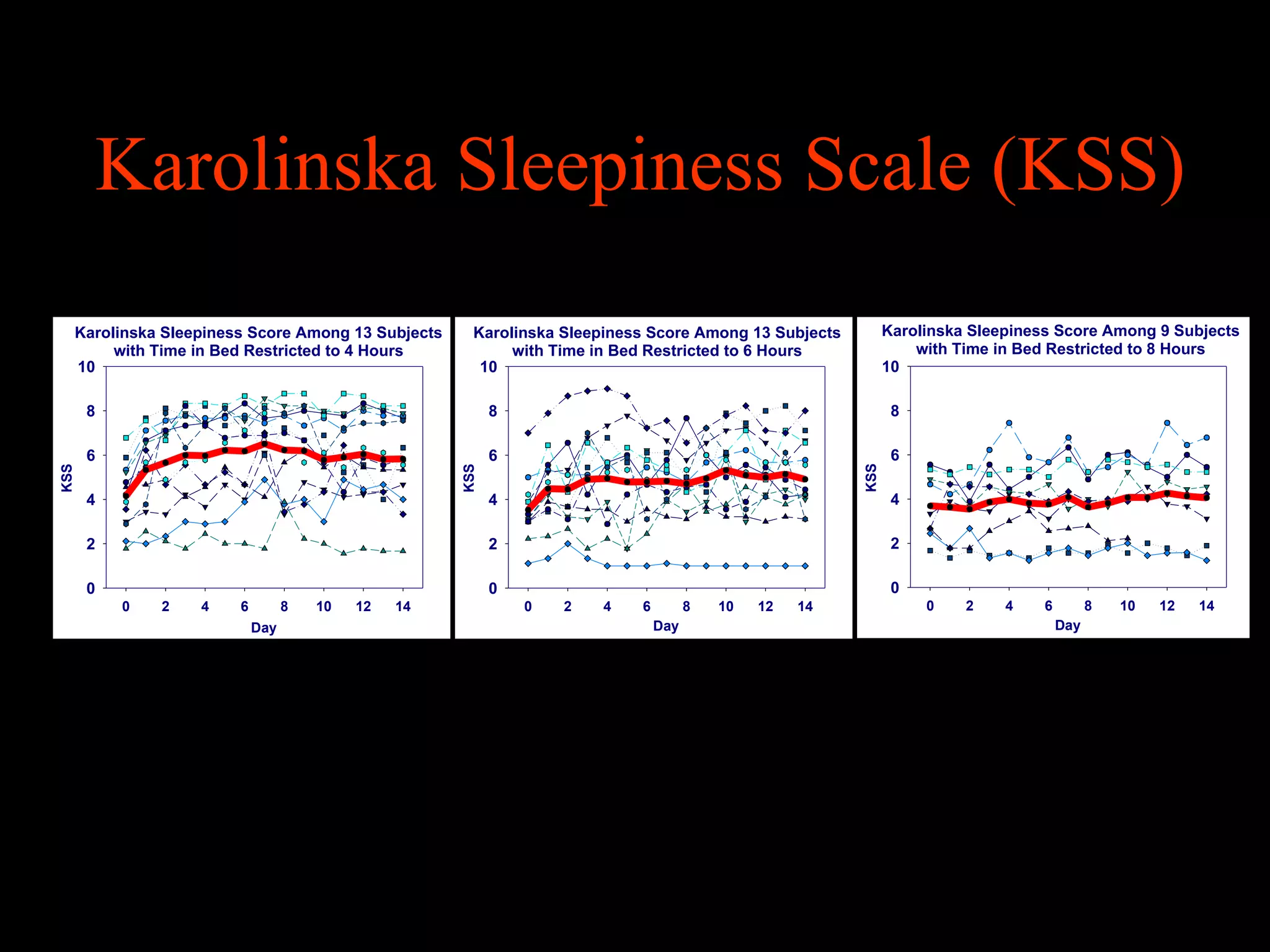
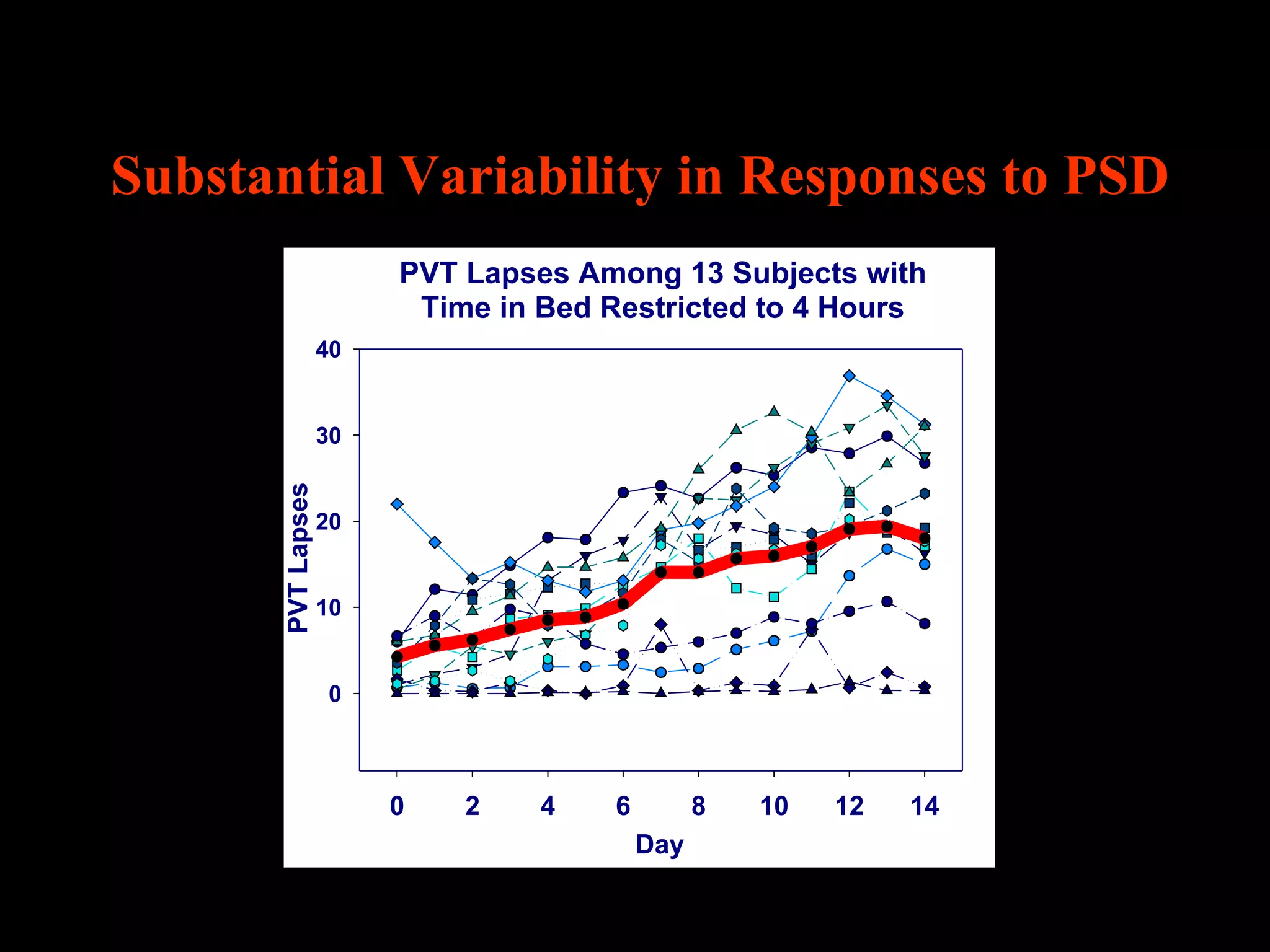
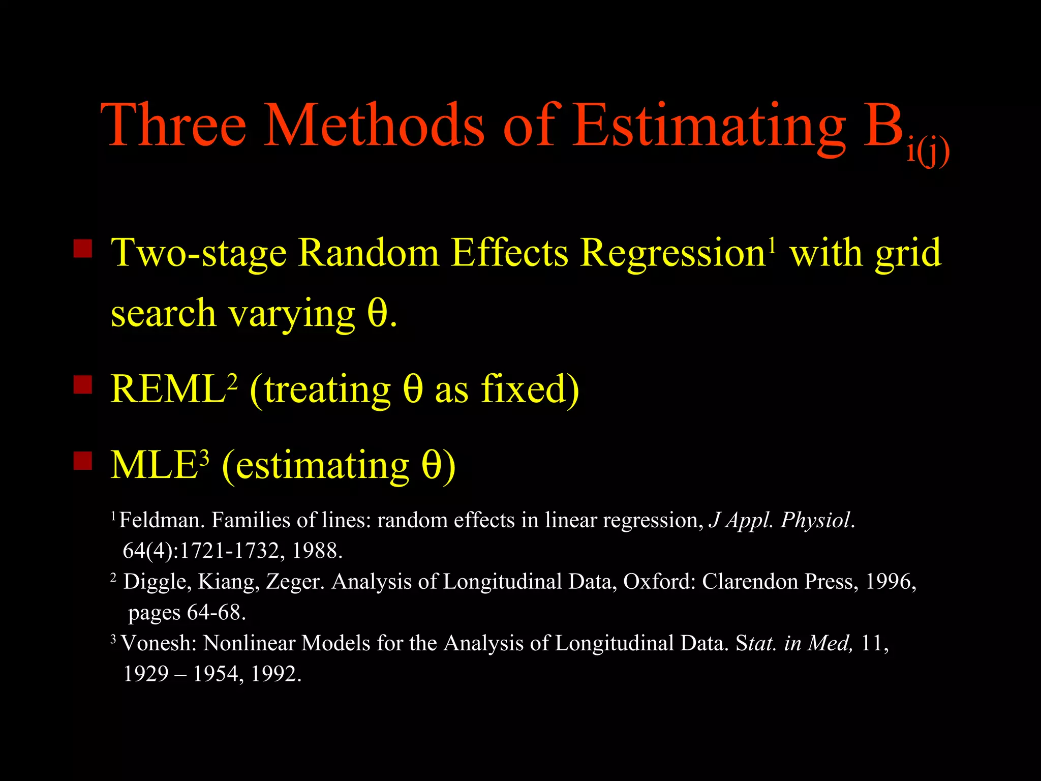
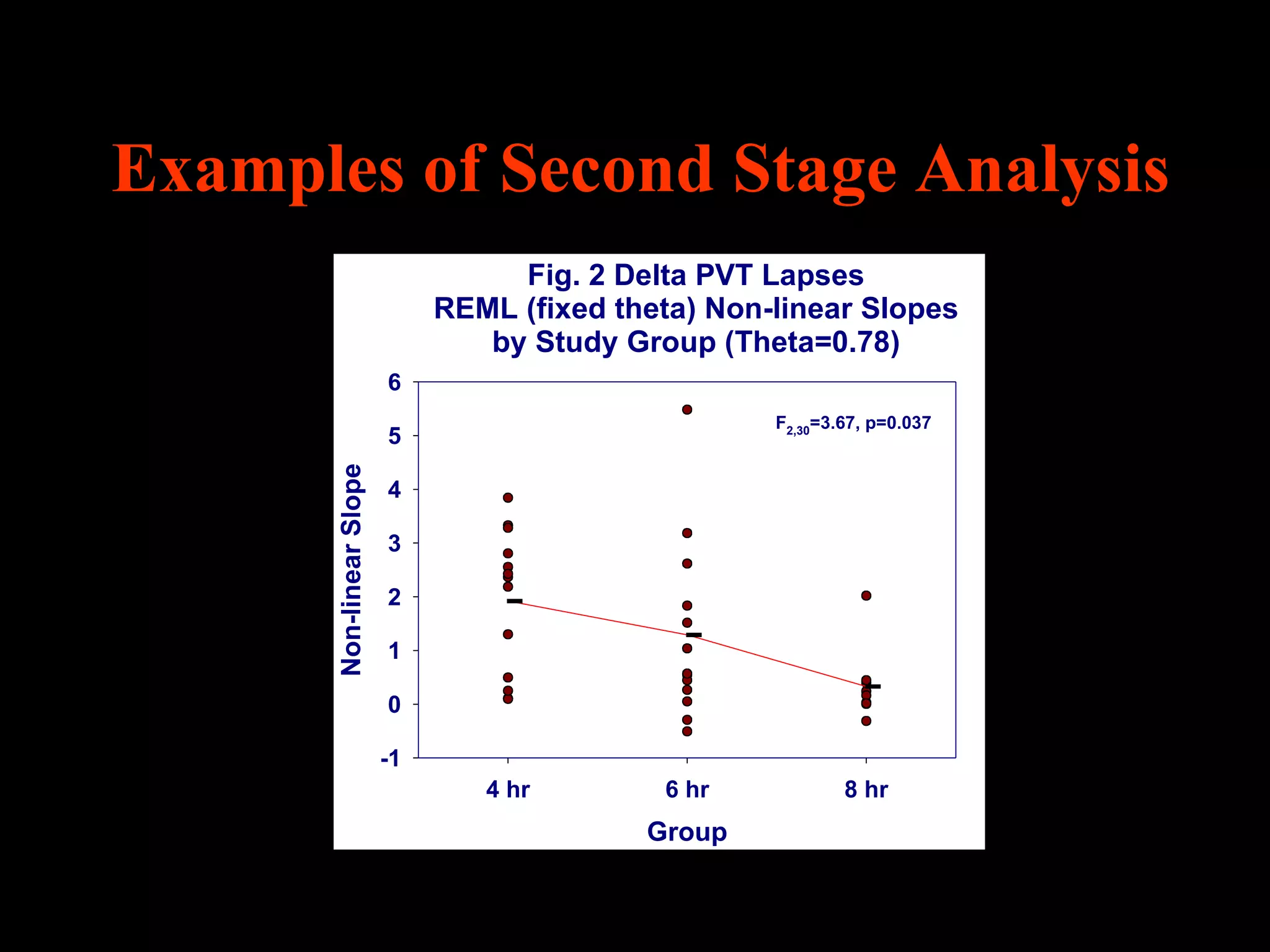
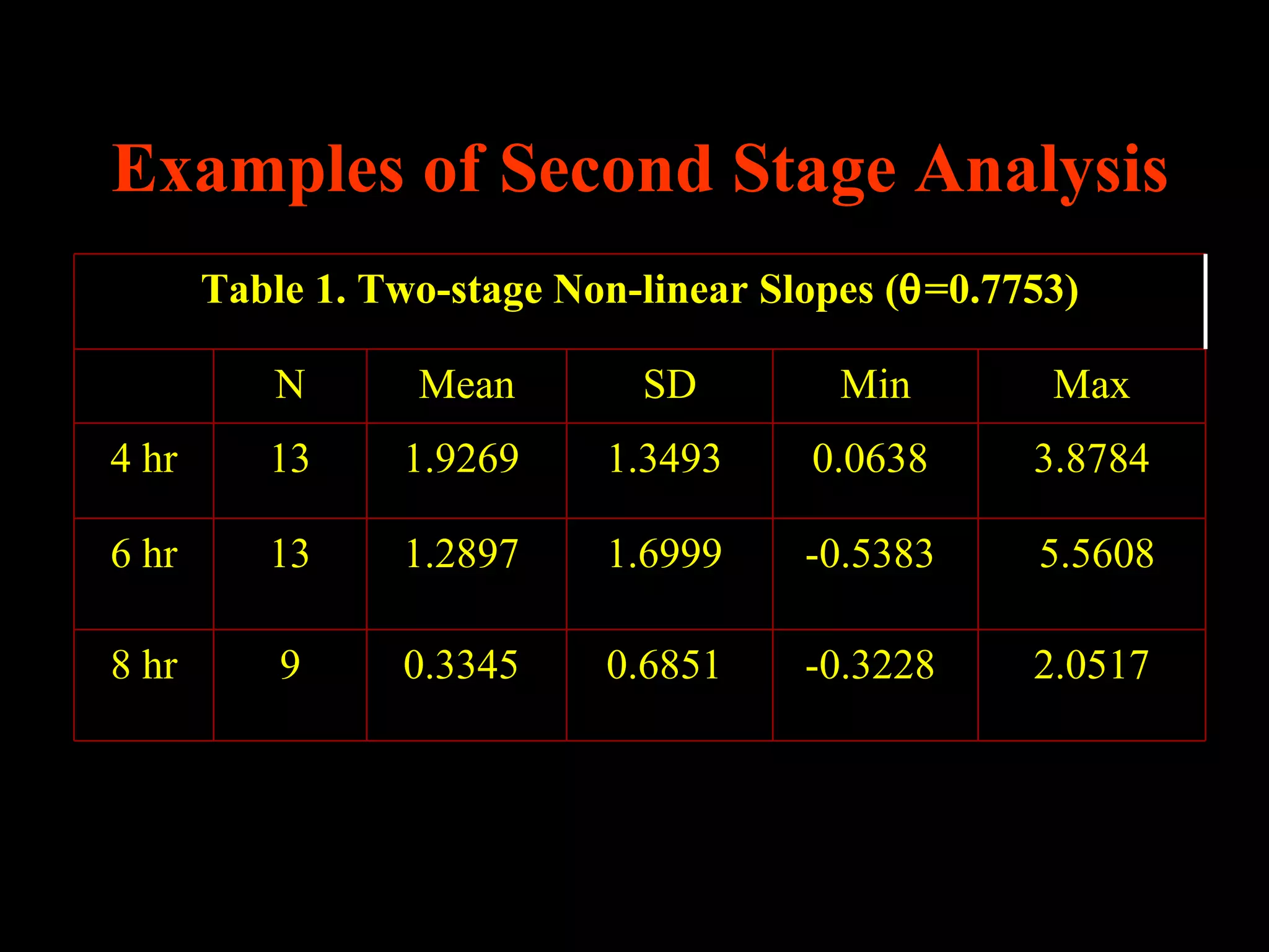
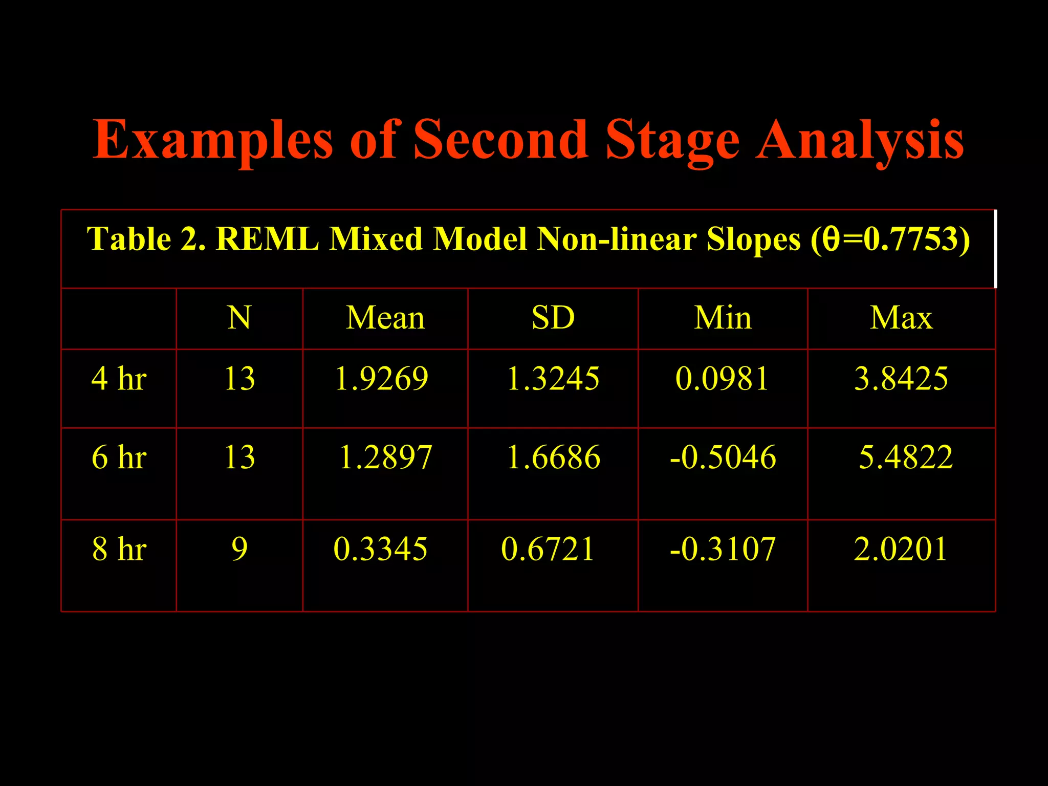
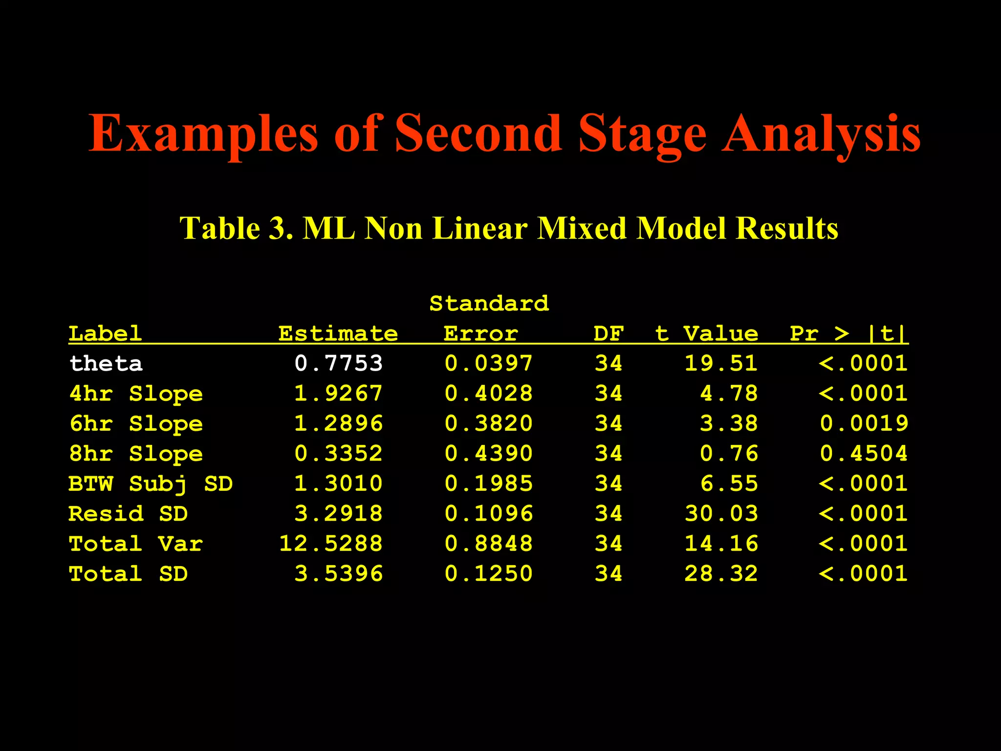
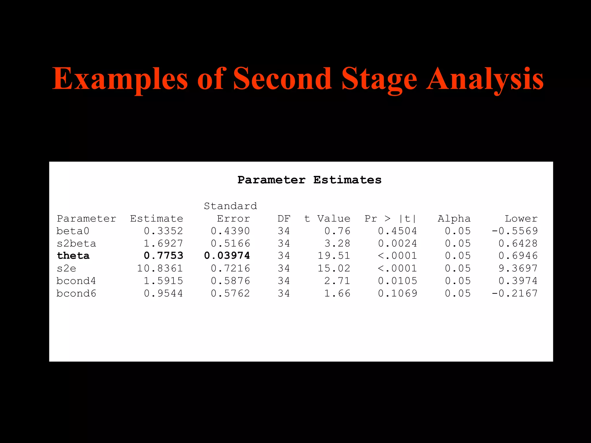
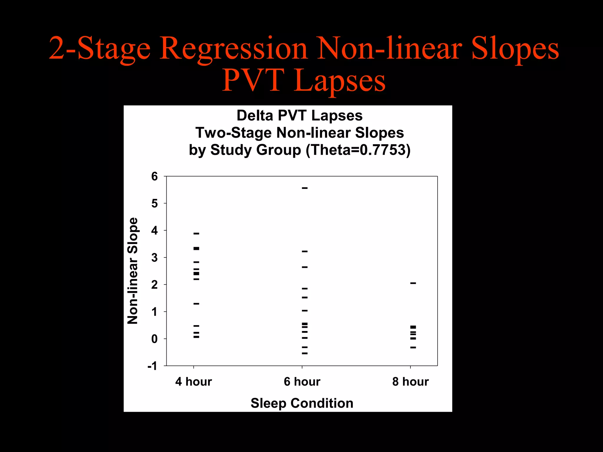
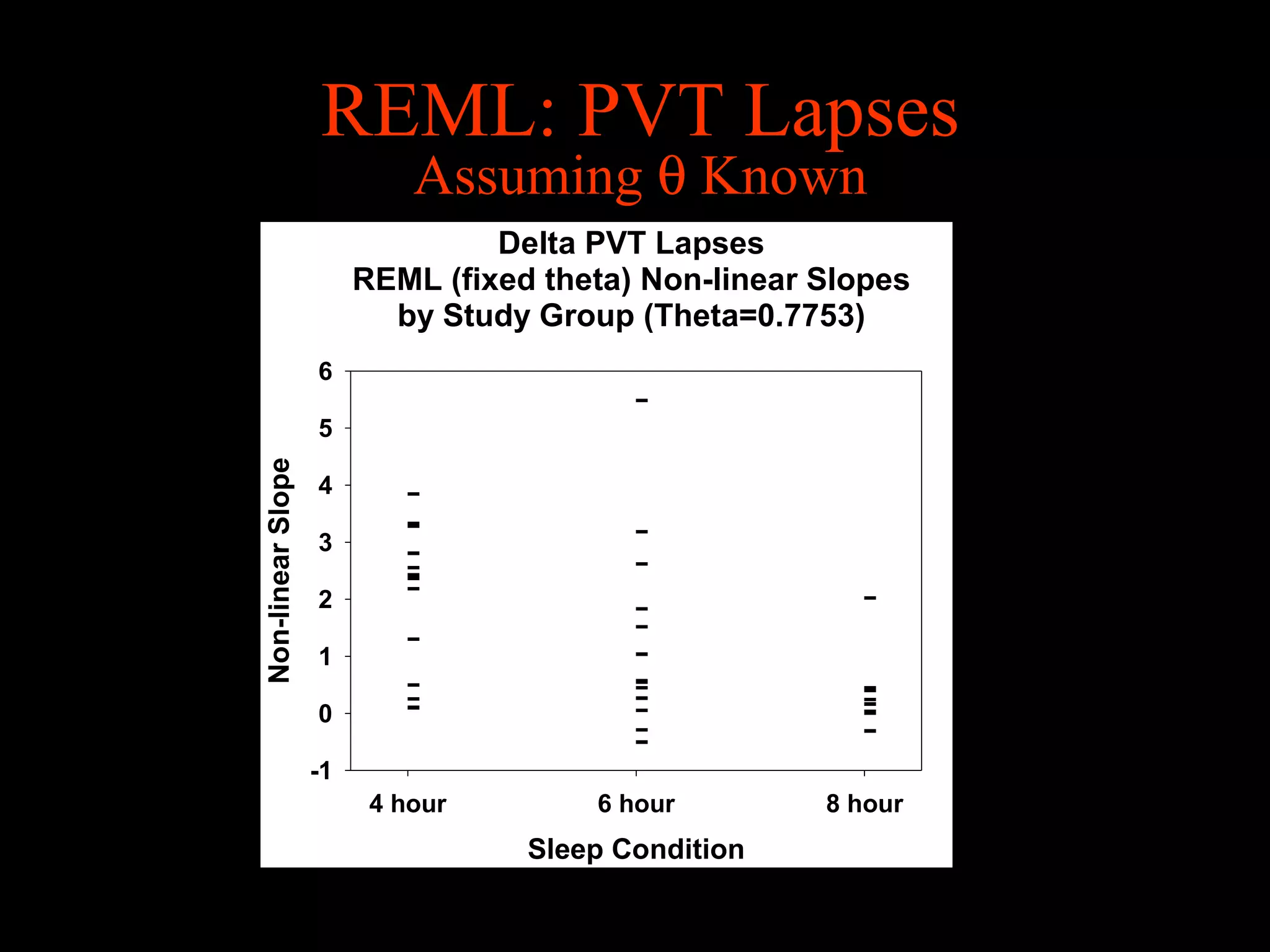
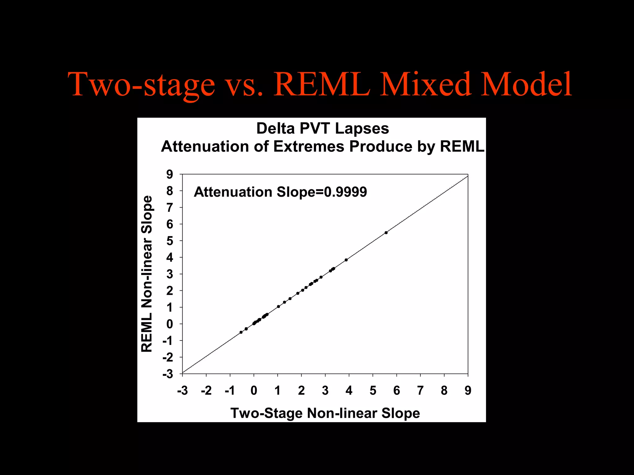
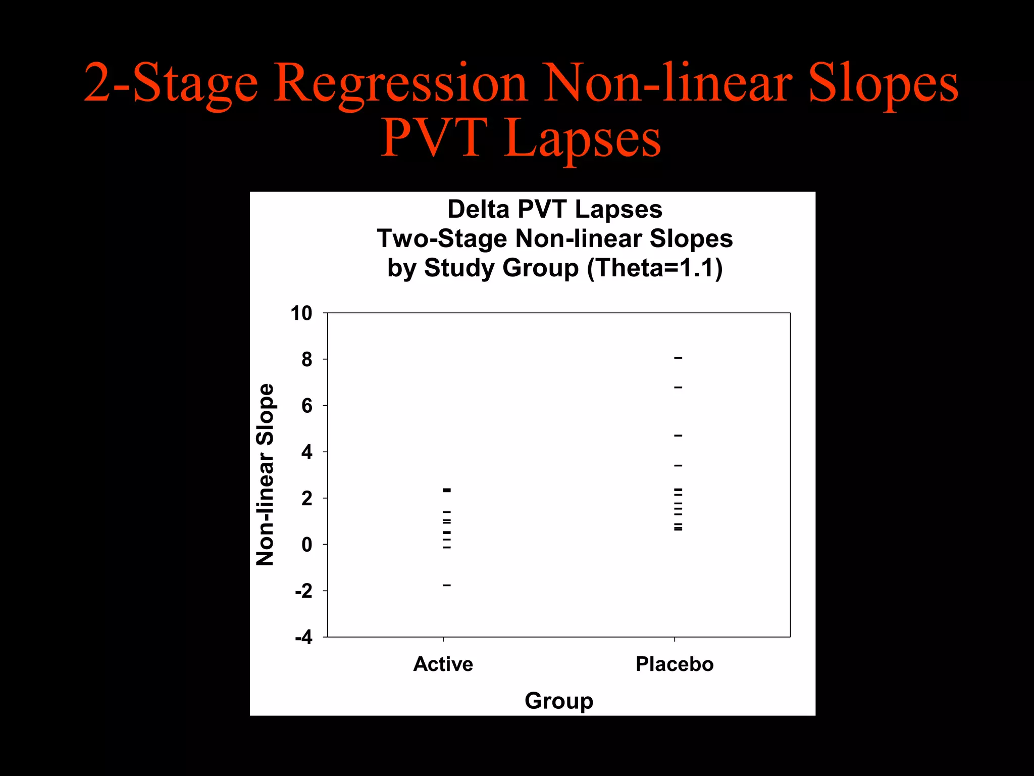
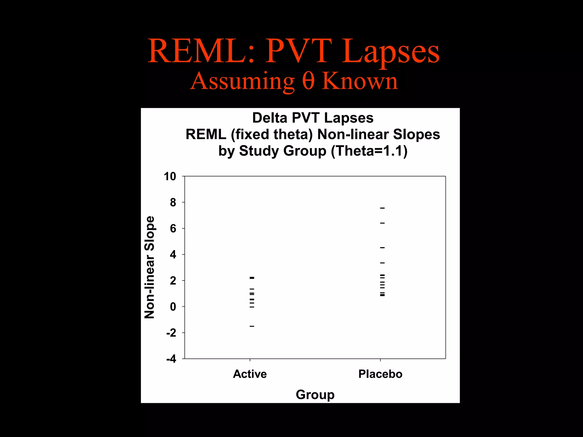
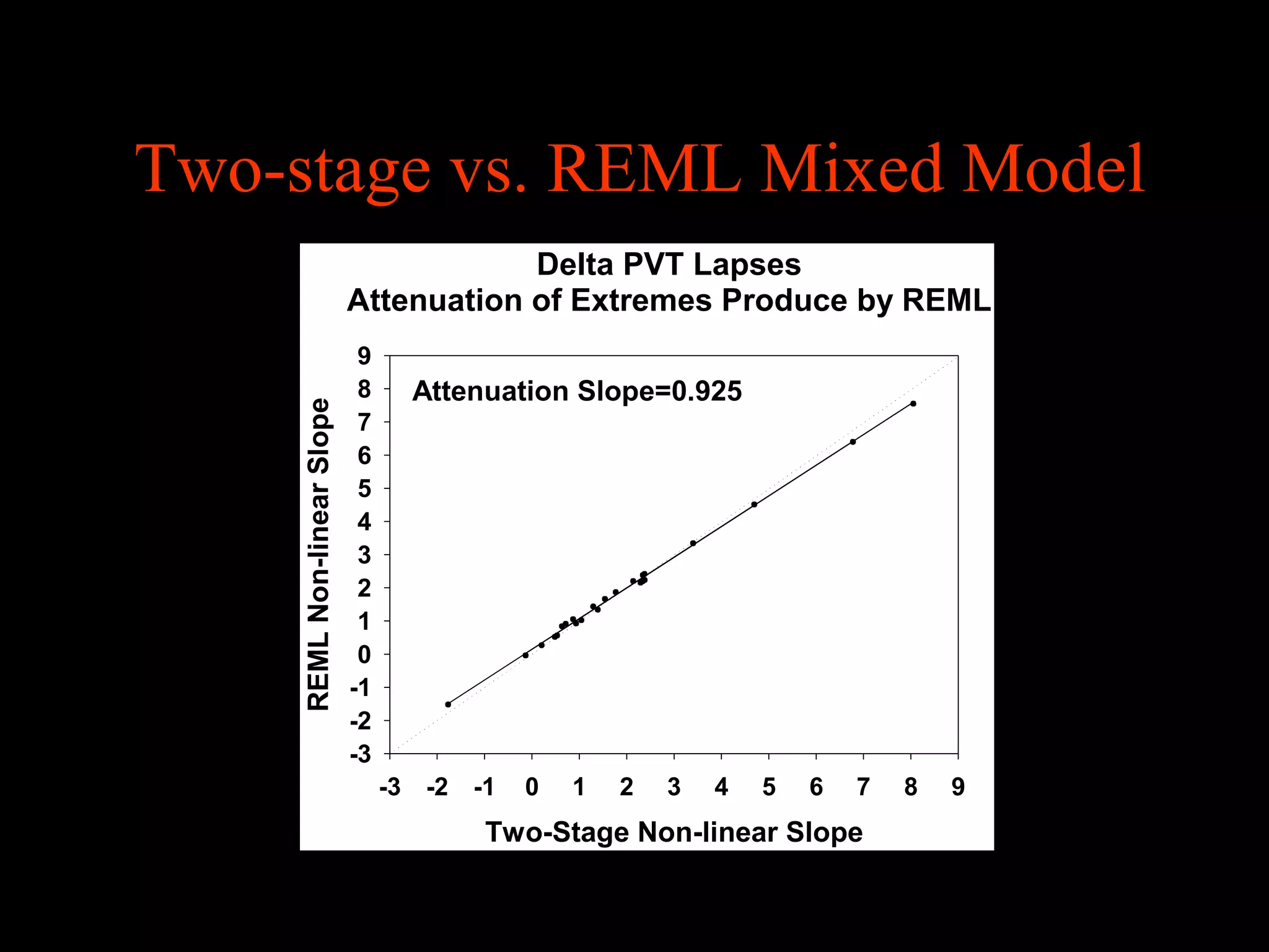
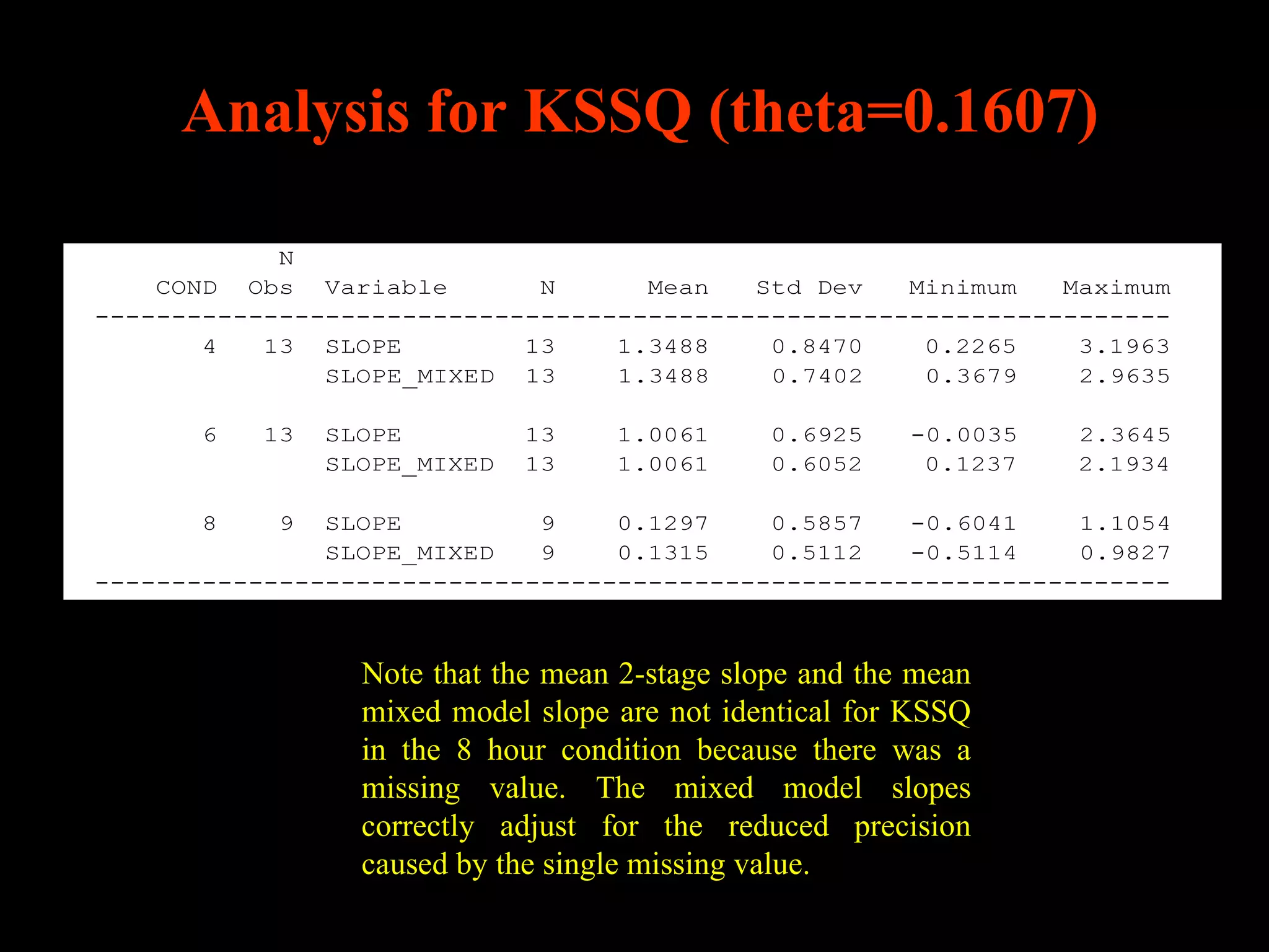
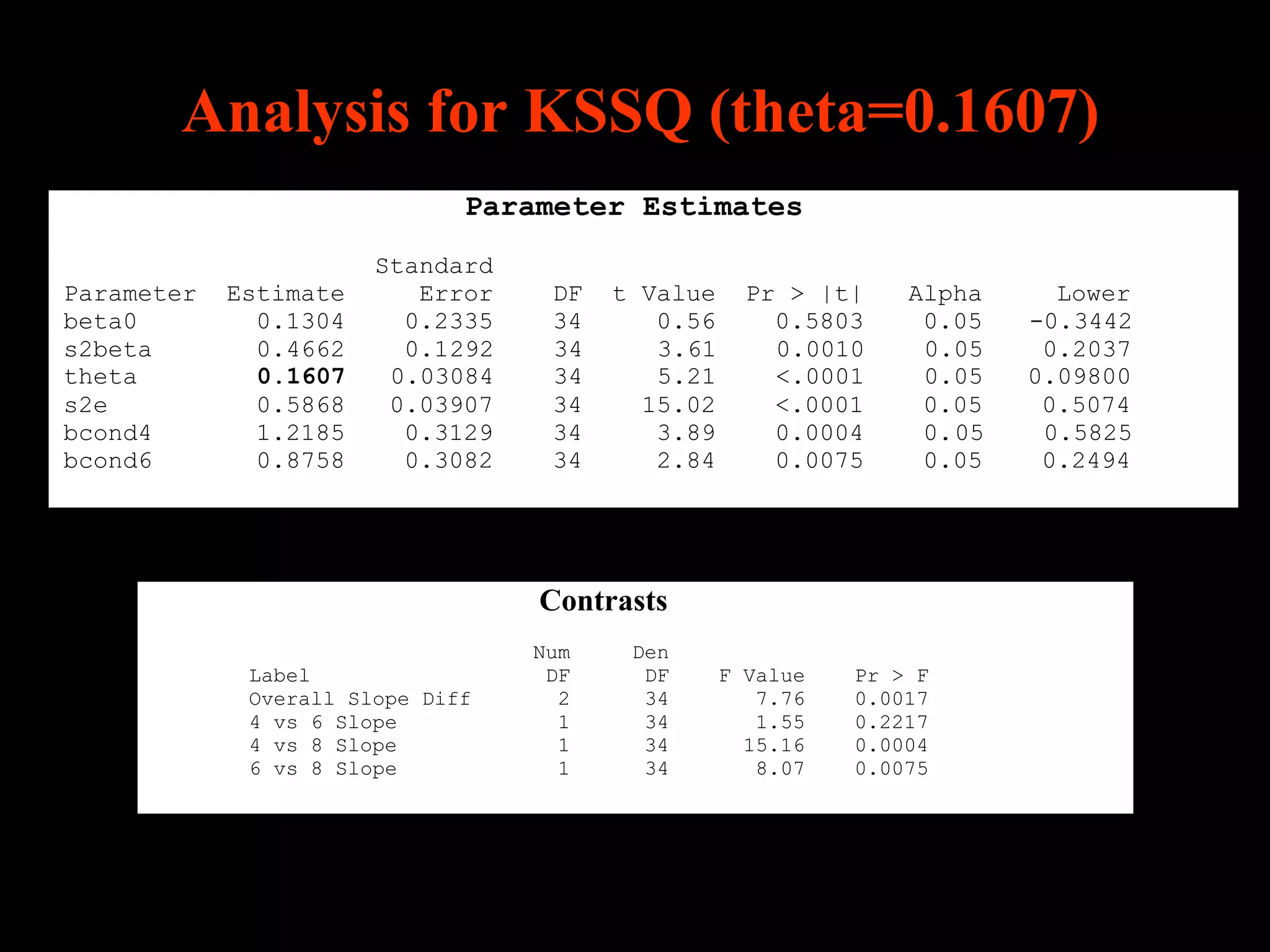
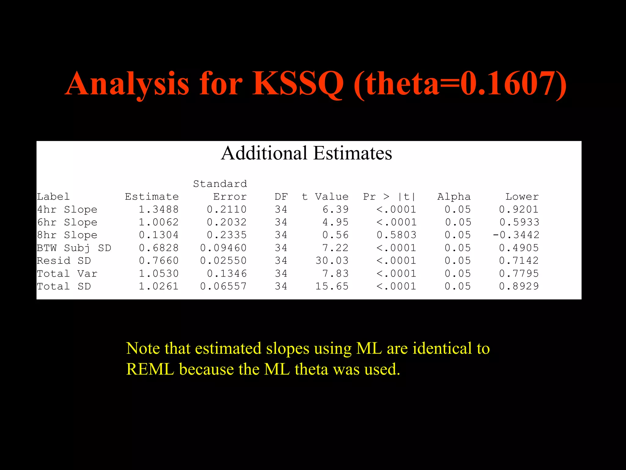
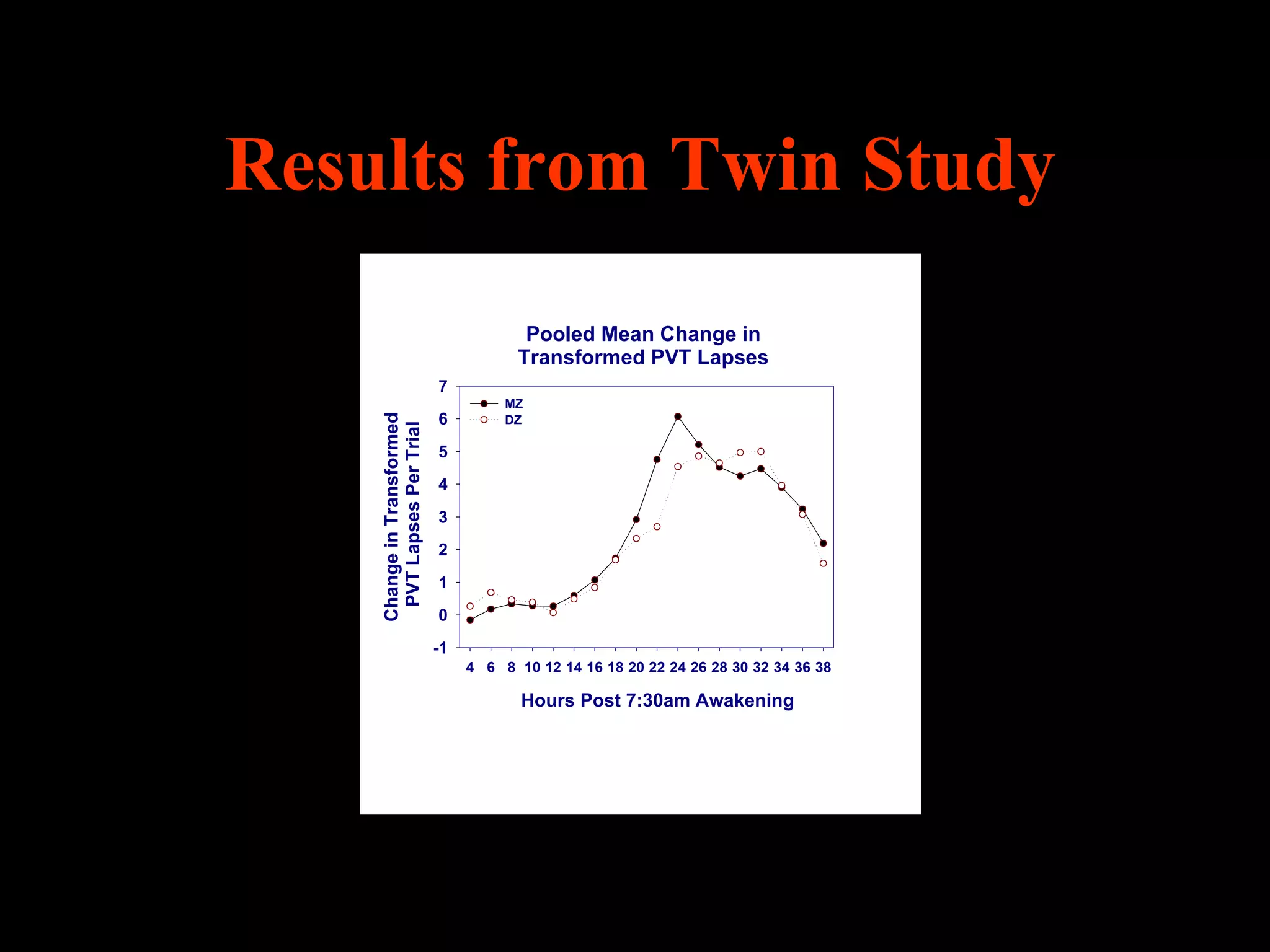
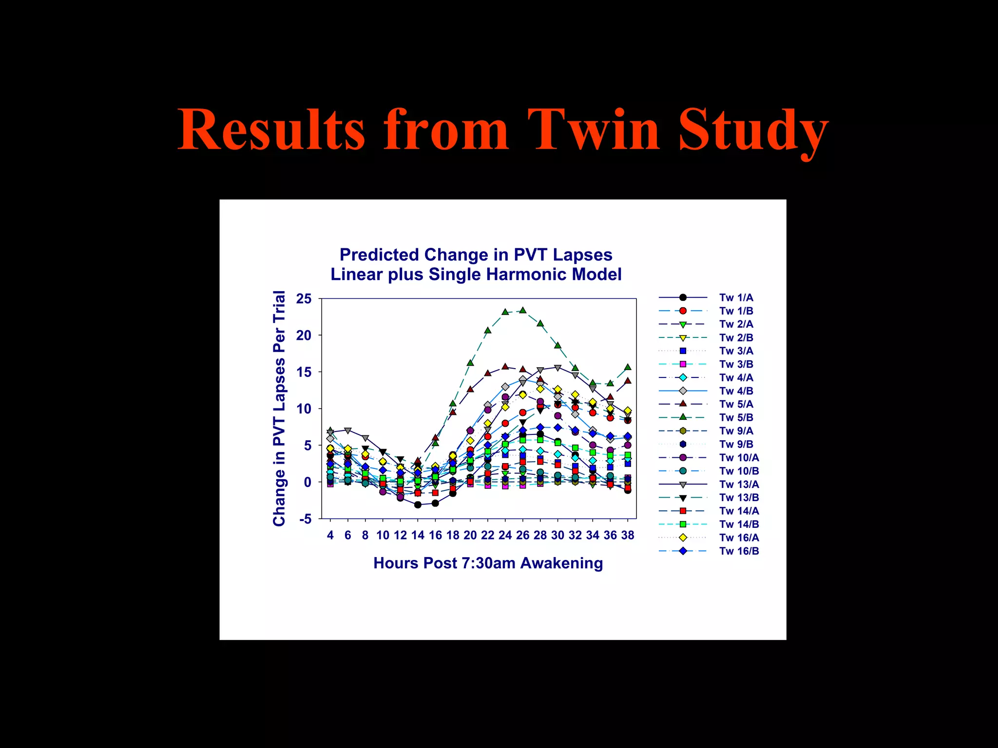
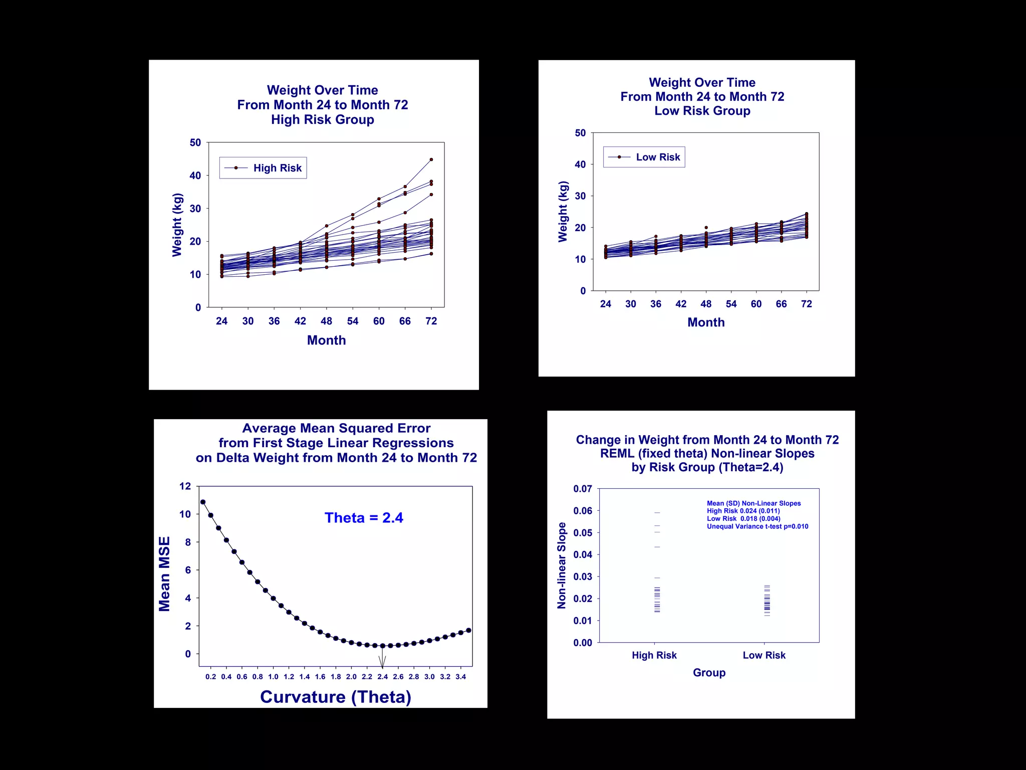
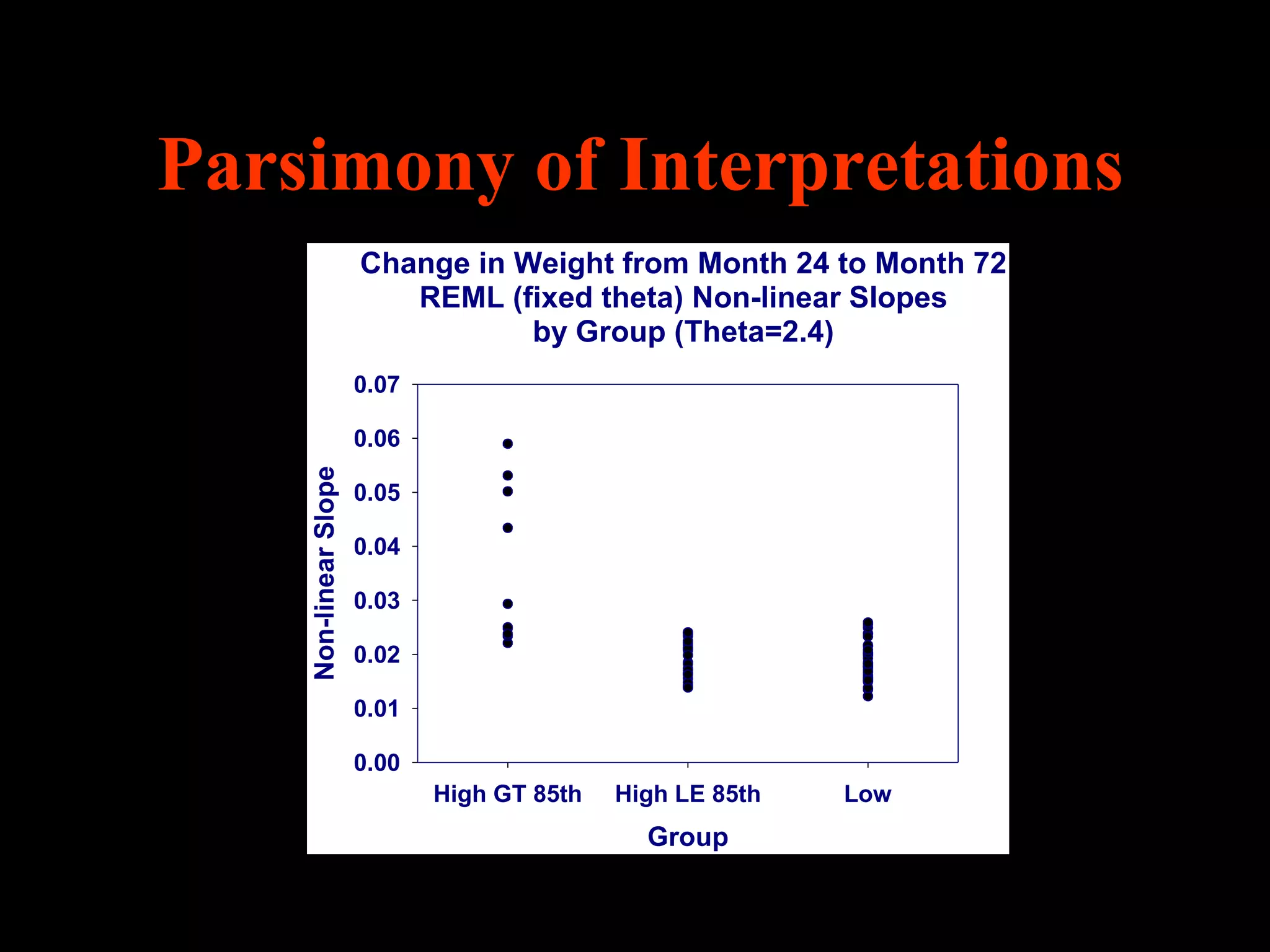
Parsimonious Statistical Modeling
  of Inter-Individual Response
 Differences to Sleep Deprivation

                   Greg Maislin
             Principal Biostatistician
       Biomedical Statistical Consulting &
Director, Biostatistics and Data Management Core
 Center for Sleep and Respiratory Neurobiology
 University of Pennsylvania School of Medicine
Acknowledgements and Thanks
   Special thanks to Dr. David F. Dinges whose experiments
    exploring the consequences of partial and total sleep
    deprivation with and without counter measures provided
    fertile ground for deep thinking about some very interesting
    statistical issues.
   To Dr. Hans Van Dongen for challenging me to be clear and
    compelling in my thinking.
   And to Bob Hachadoorian, Senior Statistical Programmer for
    his dedication in programming SAS production runs capable
    of mass processing multitudes of assessments across many
    domains in the PSD and TSD protocols.
Introduction
   Inter-individual differences in response to sleep loss
    are substantial. Sleep deprivation protocols often
    involve neurobehavioral and physiological testing
    over multiple days. There is need for conceptually
    simple, yet quantitatively valid statistical methods
    that recognize inter-individual variability and
    accommodate assay-specific non-linearity of time
    trajectories.
Intraclass Correlation Coefficient
                   (ICC)
   Between-subject variance (σbs2 )
   Within-subject (σws2) variance
   σTotal2 = σbs2 + σws2
   ICC is defined as follows to quantify trait-like
    inter-individual variability:
   ICC =      σbs2
            σbs2 + σws2
Intraclass Correlation Coefficient
                   (ICC)
   ICC varies by population since σbs2 varies by
    population.
   The magnitudes of σbs2 and σws2 should be
    interpreted, not just ICC.
   Mixed effects ANOVA can be used to estimate
    ICC-like measures that include multiple sources
    of variance and that filter out ‘fixed’ effects
    such as demographic factors and experimental
    conditions.
Evidence of Trait-Like Variance


Change in Total PVT lapses after two exposures 2-4 wks
apart of 36 h sleep deprivation.
Van Dongen HP, Kijkman M, Maislin G, Dinges D. Phenotypic aspect of
vigilance decrement during sleep deprivation. Physiologist 1999; 42:A-5.
Evidence of Trait-Like Variance
                                    PVT Transformed Lapses Linear Slopes
                                  Over 38 Hours (19 trials) of Sleep Deprivation
                                              Monozygotic Twins
                               0.5
                                      ICC = 56.0% (N=48 pairs)
                                      Var(B) = 3.51*10E-3
      PVT Transformed Lapses


                               0.4
                                      Var(W) = 2.76*10E-3
           Linear Slopes


                               0.3

                               0.2


                               0.1

                               0.0


                               -0.1
                                        2
                                       82
                                        9
                                       46
                                       37
                                       14
                                        3
                                      101
                                       64
                                      121
                                       91
                                      118
                                      109
                                       56
                                       47
                                       95
                                       22
                                       67
                                       63
                                       51
                                       27
                                       93
                                      136
                                       13
                                       17
                                      129
                                       28
                                       31
                                       42
                                       74
                                       87
                                      120
                                       62
                                       54
                                      108
                                       73
                                      103
                                       53
                                      116
                                       48
                                       49
                                       97


                                      122


                                       23


                                       78


                                       79


                                       44


                                       38
                                                      Twin Pair


        Preliminary data from Heritability of Sleep
      Homeostasis, Drs. Allan Pack and Samuel Kuna,
               Division of Sleep Medicine.
Evidence of Trait-Like Variance
                                    PVT Transformed Lapses Linear Slopes
                                  Over 38 Hours (19 trials) of Sleep Deprivation
                                               Dizygotic Twins
                               0.5
                                      ICC = 24.5% (N=30 pairs)
                                      Var(B) = 0.93*10E-3
      PVT Transformed Lapses


                               0.4
                                      Var(W) = 2.87*10E-3
           Linear Slopes


                               0.3

                               0.2


                               0.1

                               0.0


                               -0.1
                                      132
                                       98
                                      135
                                       29
                                      117
                                      142
                                      126
                                      106
                                       25
                                      128

                                       10
                                      148

                                       94

                                       41
                                        4


                                       16
                                      124


                                      127

                                        5
                                      138
                                       52
                                      134


                                      100

                                      149


                                       58
                                      113
                                      104


                                      130
                                      145

                                       57
                                                      Twin Pair
‘Test-bed’ Experiment1
   This sleep restriction experiment involved one adaptation day
    and two baseline days with 8 h sleep opportunities (TIB
    23:30–07:30), followed by randomization to 8 h, 6 h or 4 h
    periods for nocturnal sleep (TIB ending at 07:30) for 14 days.
           13 Subjects randomized to 4 hrs TIB for 14 days
           13 Subjects randomized to 6 hrs TIB for 14 days
            9 Subjects randomized to 8 hrs TIB for 14 days
   Assessments every 2 hrs during wakefulness
    1
     Van Dongen HP, Maislin G, Mullington JM, and Dinges DF. The cumulative cost
    of additional wakefulness: Dose-response effects on neurobehavioral functions and
    sleep physiology from chronic sleep restriction and total sleep restriction.
    Sleep 2003, 26(2):117-126.
Neurobehavioral Test Battery (NAB)
(1) Psychomotor vigilance task (PVT) (Dinges & Powell 1985)
(2) Probed recall memory (PRM) test that controls for reporting bias and evaluates free
    recall/retention (Dinges et al 1993)
(3) Digit symbol substitution task (DSST) assesses cognitive throughput (speed/accuracy)
(4) Time estimation task (TET)
(5) Performance evaluation and effort rating scales (PEERS) to track self monitoring,
    compensatory effort, and motivation (Dinges et al 1992)


(1) Karolinska Sleepiness Scale (KSS) (Akerstedt & Gillberg 1990)
(2) Stanford Sleepiness Sale (SSS) (Hoddes et al 1973)
(3) Visual analog scale (VAS) for mental and physical exhaustion
(4) Activation-Deactivation Checklist (AD-ACL)(Thayer 1986)
(5) Profile of Mood States (POMS) (McNair, Lorr, & Druppleman 1971)
Psychomotor vigilance task (PVT)
 Simple, high-signal-load reaction time (RT)
  test designed to evaluate the ability to sustain
  attention and respond in a timely manner to
  salient signals.
 10 minute duration
 Yields six primary metrics on the capacity for
  sustained attention and vigilance performance.
Psychomotor vigilance task (PVT)
   Frequency of lapses (RT>500 msec)
   Duration of the lapse domain (mean of 10% slowest
    reciprocal RTs)
   Optimum response times (mean of 10% fastest RTs)
   False response frequency (errors),
   Frequency of non-responses (caused by spontaneous
    sleep episodes)
   Fatigability function (slope computed from 1 minute
    bins of mean 1/RTs).
Average Daily PVT Lapses/Trial
                  PVT Lapses Among 13 Subjects with                           PVT Lapses Among 13 Subjects with                               PVT Lapses Among 9 Subjects with
                   Time in Bed Restricted to 4 Hours                           Time in Bed Restricted to 6 Hours                               Time in Bed Restricted to 8 Hours
             40                                                          50                                                          25


                                                                         40                                                          20
             30

                                                                         30                                                          15
PVT Lapses


                                                                                                                        PVT Lapses
                                                            PVT Lapses
             20
                                                                         20                                                          10
             10
                                                                         10                                                           5

             0
                                                                          0                                                           0


                  0   2    4   6         8   10   12   14                     0   2    4   6         8   10   12   14                     0      2    4    6         8   10   12   14
                                   Day                                                         Day                                                             Day
Karolinska Sleepiness Scale (KSS)
                           Karolinska Sleepiness Scale (KSS)
  Place the X next to the ONE statement that best describes your SLEEPINESS
  during the PREVIOUS 5 MINUTES. You may also use the intermediate steps.

  X
  __    1.   very alert
  __    2.
  __    3.   alert, normal level
  __    4.
  __    5.   neither alert nor sleepy
  __    6.
  __    7.   sleepy, but no effort to keep awake
  __    8.
  __    9.   very sleepy, great effort to keep awake, fighting sleep

  Use {UP/ DOWN} cursor keys to move      X   block, then press {ENTER}
Karolinska Sleepiness Scale (KSS)
      Karolinska Sleepiness Score Among 13 Subjects      Karolinska Sleepiness Score Among 13 Subjects          Karolinska Sleepiness Score Among 9 Subjects
           with Time in Bed Restricted to 4 Hours             with Time in Bed Restricted to 6 Hours                with Time in Bed Restricted to 8 Hours
      10                                                  10                                                    10

       8                                                     8                                                   8

       6                                                     6                                                   6


                                                                                                          KSS
KSS


                                                       KSS

       4                                                     4                                                   4

       2                                                     2                                                   2

       0                                                     0                                                   0
           0    2    4    6         8   10   12   14             0   2   4   6         8   10   12   14              0    2    4    6         8   10   12   14
                              Day                                                Day                                                    Day
Observations
   For the subjective measure, end-of-study values
    depend heavily on baseline values.
   The objective measure increased linearly throughout
    the PSD protocol.
   The increase in the subjective measure was non-
    linear with decelerating increases. Most of the
    increase was very early.
   There was substantial variability among subjects in
    both objective and subjective responses to PSD.
Substantial Variability in Responses to PSD
                        PVT Lapses Among 13 Subjects with
                         Time in Bed Restricted to 4 Hours
                   40


                   30
      PVT Lapses


                   20


                   10


                   0


                        0   2    4   6         8   10   12   14
                                         Day
Statistical Approaches
                     for Growth Curves
   Classical repeated measures analysis fails to recognize individual
    response variance. It is a model for the mean response with no
    recognition of true biological variability among subjects in the
    magnitudes of their response.
   Mixed effects models for each individual observation include
    random subject effects and can allow for a variety of covariance
    structures that can reflect many different assumptions concerning
    the nature of within subject correlations overtime (e.g. AR(1)).
    Although theoretically appealing, concern has been raised about
    the robustness of these models1. They also require sophisticated
    statistical approaches that may not be immediately accessible to all
    researchers.
    1
     Ahnn, Tonidandel, and Overall. Issues in use of Proc.Mixed to test the significance of
    treatment effects in controlled clinical trials. J of Biopharm Stat 10(2):265-286, 2000
Standard Two Stage (STS) regression
   Using simple linear regression, a slope (and intercept) for each
    subject are determined at the first stage. Second stage group
    comparisons are made by comparing mean slopes.
   STS gives each subject’s first stage slope estimate equal
    weight, which is not appropriate if the sample size or layout of
    time values varies widely among subjects.
   STS disguises residual error, pooling it with between-subject
    variance and biasing the latter upward. If residual variance is
    small or the numerical values of variance components are not
    themselves of interest, this is not a problem.
Standard Two Stage (STS) regression (cont.)
   STS does not account for the covariance between
    slopes and intercepts.
   Parsimony: It is desirable to reduce the response
    curve to a single number (eliminating the intercept).
   Slopes assume constant accumulations of deficit over
    time. However, accumulation of deficits can be
    decelerating or accelerating.
Mixed linear model determination of slopes
   The simultaneous determination of subject specific
    slopes using maximum likelihood incorporates the
    assumption that the slopes are normally distributed with
    condition-specific mean values and a common variance.
   STS does not make this assumption, computing each
    subject-specific slope independently from all other
    subjects (robustness?).
Proposed Model: Two-Stage Non-Linear
           Mixed Model Regression

               ∆(t)i(j) = Bi(j) · tθ + ε(t)i(j)
   ∆(t)i(j) = performance deficit for subject i in group j at
    time t
   θ is a curvature parameter reflecting the nature of
    non-linearity of growth in deficits
   Bi(j) are subject-specific “non-linear” slopes
   ε(t)i(j) are residual errors.
Reference
   Van Dongen HPA, Maislin G, Dinges DF.
    Dealing with inter-individual differences in
    the temporal dynamics of fatigue and
    performance: Importance and techniques.
    Aviat Space Environ Med 2004: 75:A147–
    A154.
Proposed Model: Two-Stage Non-Linear
            Mixed Model Regression

   The (non-linear) slopes are combinations of group
    specific mean values and random effects reflecting
    individual susceptibilities to the deprivation challenge.
   Bi(j) = β j + bi(j)
    βj is the mean response in group j
    bi(j) ~ Normal(0, σ2b).
    σ2b is a subject specific variance contribution.
    Bi(j) ~ Normal(βj,, σ2b ).
Three Methods of Estimating Bi(j)
   Two-stage Random Effects Regression1 with grid
    search varying θ.
   REML2 (treating θ as fixed)
   MLE3 (estimating θ)
    1
      Feldman. Families of lines: random effects in linear regression, J Appl. Physiol.
      64(4):1721-1732, 1988.
    2
      Diggle, Kiang, Zeger. Analysis of Longitudinal Data, Oxford: Clarendon Press, 1996,
       pages 64-68.
    3
      Vonesh: Nonlinear Models for the Analysis of Longitudinal Data. Stat. in Med, 11,
      1929 – 1954, 1992.
Two-stage Random Effects Regression
       with Grid search varying θ
 Simple  linear regression for each subject
  varying θ from 0.1 to 2.0.
 The θ that minimizes the average MSE is
  selected.
Two-stage Random Effects Regression
    with Grid search varying θ
                      Fig. 1 Grid Search Over Average MSE
                       from First Stage Linear Regressions
                           on Delta PVT Lapses Values
                 24

                 22
                                                          Theta = 0.78
                 20
      Mean MSE


                 18

                 16

                 14

                 12

                 10
                      0.1 0.2 0.3 0.4 0.5 0.6 0.7 0.8 0.9 1.0 1.1 1.2 1.3 1.4 1.5 1.6 1.7 1.8 1.9 2.0


                                       Curvature (Theta)
REML Mixed Linear Model (fixed θ)
   The 2-stage approach disguises residual error, pooling
    it with between-subject variance and biasing the latter
    upward (compare SD’s in Table 1 and Table 2).
   Conditional on the value of the optimal θ obtained
    from the grid search, the model is no longer non-linear.
   When θ is assumed known, a mixed linear model can
    be used to simultaneously derive subject specific
    slopes (e.g., SAS Proc Mixed).
ML Mixed Non-Linear Model
        (simultaneous estimation of θ)
   Has greatest theoretical appeal.
   Requires specialized software
    (e.g., SAS Proc NLMIXED).
    Model sometimes does not converge.
    More precise estimate of θ (Table 3).
Examples of Second Stage Analysis
                                    Fig. 2 Delta PVT Lapses
                               REML (fixed theta) Non-linear Slopes
                                  by Study Group (Theta=0.78)
                          6
                                                      F2,30=3.67, p=0.037
                          5
       Non-linear Slope


                          4

                          3

                          2

                          1

                          0

                          -1
                                  4 hr        6 hr            8 hr
                                             Group
Examples of Second Stage Analysis
       Table 1. Two-stage Non-linear Slopes (θ=0.7753)

          N       Mean        SD         Min        Max
4 hr      13     1.9269     1.3493     0.0638      3.8784

6 hr      13     1.2897     1.6999     -0.5383     5.5608

8 hr       9     0.3345     0.6851     -0.3228     2.0517
Examples of Second Stage Analysis
Table 2. REML Mixed Model Non-linear Slopes (θ=0.7753)

        N      Mean        SD        Min       Max
4 hr    13     1.9269    1.3245    0.0981     3.8425

6 hr    13     1.2897    1.6686    -0.5046     5.4822

8 hr    9      0.3345    0.6721    -0.3107    2.0201
Examples of Second Stage Analysis
       Table 3. ML Non Linear Mixed Model Results

                         Standard
Label         Estimate    Error     DF   t Value   Pr > |t|
theta          0.7753     0.0397    34     19.51     <.0001
4hr Slope      1.9267     0.4028    34      4.78     <.0001
6hr Slope      1.2896     0.3820    34      3.38     0.0019
8hr Slope      0.3352     0.4390    34      0.76     0.4504
BTW Subj SD    1.3010     0.1985    34      6.55     <.0001
Resid SD       3.2918     0.1096    34     30.03     <.0001
Total Var     12.5288     0.8848    34     14.16     <.0001
Total SD       3.5396     0.1250    34     28.32     <.0001
Examples of Second Stage Analysis

                            Parameter Estimates

                       Standard
Parameter   Estimate     Error    DF   t Value   Pr > |t|   Alpha     Lower
beta0         0.3352    0.4390    34      0.76     0.4504    0.05   -0.5569
s2beta        1.6927    0.5166    34      3.28     0.0024    0.05    0.6428
theta         0.7753   0.03974    34     19.51     <.0001    0.05    0.6946
s2e          10.8361    0.7216    34     15.02     <.0001    0.05    9.3697
bcond4        1.5915    0.5876    34      2.71     0.0105    0.05    0.3974
bcond6        0.9544    0.5762    34      1.66     0.1069    0.05   -0.2167
2-Stage Regression Non-linear Slopes
            PVT Lapses
                                     Delta PVT Lapses
                                Two-Stage Non-linear Slopes
                               by Study Group (Theta=0.7753)
                        6

                        5
     Non-linear Slope


                        4

                        3

                        2

                        1

                        0

                        -1
                             4 hour        6 hour        8 hour
                                       Sleep Condition
REML: PVT Lapses
                            Assuming θ Known
                                 Delta PVT Lapses
                        REML (fixed theta) Non-linear Slopes
                          by Study Group (Theta=0.7753)
                   6

                   5
Non-linear Slope


                   4

                   3

                   2

                   1

                   0

                   -1
                         4 hour        6 hour         8 hour
                                   Sleep Condition
Two-stage vs. REML Mixed Model
                                        Delta PVT Lapses
                            Attenuation of Extremes Produce by REML
                             9
                             8     Attenuation Slope=0.9999
    REML Non-linear Slope


                             7
                             6
                             5
                             4
                             3
                             2
                             1
                             0
                            -1
                            -2
                            -3
                                 -3 -2 -1   0   1   2   3   4   5   6   7   8   9
                                        Two-Stage Non-linear Slope
2-Stage Regression Non-linear Slopes
            PVT Lapses
                                    Delta PVT Lapses
                              Two-Stage Non-linear Slopes
                               by Study Group (Theta=1.1)
                         10

                         8
      Non-linear Slope


                         6

                         4

                         2

                         0

                         -2

                         -4
                                Active           Placebo
                                         Group
REML: PVT Lapses
                        Assuming θ Known
                                 Delta PVT Lapses
                        REML (fixed theta) Non-linear Slopes
                           by Study Group (Theta=1.1)
                   10

                   8
Non-linear Slope


                   6

                   4

                   2

                   0

                   -2

                   -4
                              Active            Placebo
                                       Group
Two-stage vs. REML Mixed Model
                                        Delta PVT Lapses
                            Attenuation of Extremes Produce by REML
                             9
                             8     Attenuation Slope=0.925
    REML Non-linear Slope


                             7
                             6
                             5
                             4
                             3
                             2
                             1
                             0
                            -1
                            -2
                            -3
                                 -3 -2 -1   0   1   2   3   4   5   6   7   8   9
                                        Two-Stage Non-linear Slope
Analysis for KSSQ (theta=0.1607)

            N
    COND Obs Variable        N      Mean   Std Dev   Minimum   Maximum
----------------------------------------------------------------------
       4   13 SLOPE         13    1.3488    0.8470    0.2265    3.1963
               SLOPE_MIXED 13     1.3488    0.7402    0.3679    2.9635

      6   13   SLOPE         13    1.0061      0.6925    -0.0035   2.3645
               SLOPE_MIXED   13    1.0061      0.6052     0.1237   2.1934

      8    9   SLOPE         9    0.1297    0.5857   -0.6041    1.1054
               SLOPE_MIXED   9    0.1315    0.5112   -0.5114    0.9827
----------------------------------------------------------------------


                 Note that the mean 2-stage slope and the mean
                 mixed model slope are not identical for KSSQ
                 in the 8 hour condition because there was a
                 missing value. The mixed model slopes
                 correctly adjust for the reduced precision
                 caused by the single missing value.
Analysis for KSSQ (theta=0.1607)
                              Parameter Estimates
                       Standard
Parameter   Estimate      Error    DF   t Value     Pr > |t|    Alpha     Lower
beta0         0.1304     0.2335    34      0.56       0.5803     0.05   -0.3442
s2beta        0.4662     0.1292    34      3.61       0.0010     0.05    0.2037
theta         0.1607    0.03084    34      5.21       <.0001     0.05   0.09800
s2e           0.5868    0.03907    34     15.02       <.0001     0.05    0.5074
bcond4        1.2185     0.3129    34      3.89       0.0004     0.05    0.5825
bcond6        0.8758     0.3082    34      2.84       0.0075     0.05    0.2494


                                  Contrasts
                                  Num    Den
             Label                 DF     DF      F Value   Pr > F
             Overall Slope Diff     2     34         7.76   0.0017
             4 vs 6 Slope           1     34         1.55   0.2217
             4 vs 8 Slope           1     34        15.16   0.0004
             6 vs 8 Slope           1     34         8.07   0.0075
Analysis for KSSQ (theta=0.1607)
                             Additional Estimates
                         Standard
Label         Estimate      Error   DF   t Value   Pr > |t|   Alpha     Lower
4hr Slope       1.3488     0.2110   34      6.39     <.0001    0.05    0.9201
6hr Slope       1.0062     0.2032   34      4.95     <.0001    0.05    0.5933
8hr Slope       0.1304     0.2335   34      0.56     0.5803    0.05   -0.3442
BTW Subj SD     0.6828    0.09460   34      7.22     <.0001    0.05    0.4905
Resid SD        0.7660    0.02550   34     30.03     <.0001    0.05    0.7142
Total Var       1.0530     0.1346   34      7.83     <.0001    0.05    0.7795
Total SD        1.0261    0.06557   34     15.65     <.0001    0.05    0.8929


              Note that estimated slopes using ML are identical to
              REML because the ML theta was used.
Results from Twin Study
                                         Pooled Mean Change in
                                        Transformed PVT Lapses
                            7
                                      MZ
                            6
    Change in Transformed
     PVT Lapses Per Trial             DZ

                            5
                            4
                            3
                            2
                            1
                            0
                            -1
                                 4 6 8 10 12 14 16 18 20 22 24 26 28 30 32 34 36 38

                                        Hours Post 7:30am Awakening
Results from Twin Study

E(θ it) =
β i0 + β i1*t + ai*cos(2*Π*t/24) + bi*sin(2*Π*t/24)
Results from Twin Study
                                          Predicted Change in PVT Lapses
   Change in PVT Lapses Per Trial        Linear plus Single Harmonic Model
                                    25                                                        Tw   1/A
                                                                                              Tw   1/B
                                                                                              Tw   2/A
                                    20                                                        Tw   2/B
                                                                                              Tw   3/A
                                                                                              Tw   3/B
                                    15                                                        Tw   4/A
                                                                                              Tw   4/B
                                                                                              Tw   5/A
                                    10
                                                                                              Tw   5/B
                                                                                              Tw   9/A
                                    5                                                         Tw   9/B
                                                                                              Tw   10/A
                                                                                              Tw   10/B
                                    0                                                         Tw   13/A
                                                                                              Tw   13/B
                                                                                              Tw   14/A
                                    -5                                                        Tw   14/B
                                         4 6 8 10 12 14 16 18 20 22 24 26 28 30 32 34 36 38   Tw   16/A
                                                                                              Tw   16/B
                                                Hours Post 7:30am Awakening
Results from Twin Study
                Heritability Indices Classical Approach
                                  PVT Linear Slopes
                     Monozygotic Twins               Dizygotic Twins

              σ 2B      σ 2W   σ 2T   ICC     σ 2B   σ 2W     σ 2T     ICC      h2
Transformed                                                                    0.63
   Lapses     3.51     2.76    6.27   0.560   0.93   2.87    3.80      0.245
                                                                                  1
An Application in Another Area
   Berkowitz RI, Stallings VA, Maislin G, Stunkard AJ.
    Growth of children at high risk for obesity during the
    first six years: Implications for prevention. American
    Journal of Clinical Nutrition. Am J Clinical Nutrition
    2005;81:140–6.
   Body size and composition of high and low risk
    groups were measured repeatedly from 3 mo. to 6 yrs
    of age at CHOP. Subjects included 33 children at
    high risk for and 37 children at lower risk for obesity
    on the basis of mothers’ overweight1
    1
        high risk mean (SD) BMI = 30.2 (4.2), low risk mothers’ BMI = 19.5 (1.1).
An Application in Another Area
    At year 2, there were no differences between high
     and low risk groups in any measure of body size
     and composition1
    (Energy intake and sucking behaviors at Month 3
     were predictive of 2 year weight in both groups.)
     1
       Stunkard AJ, Berkowitz RI, Schoeller D, Maislin G, Stallings VA. Predictors of body size in the
     first 2 years of life: a high-risk study of human obesity. International Journal of Obesity 2004
     1-11.
Weight Over Time
                                         Weight Over Time                                                                         From Month 24 to Month 72
                                     From Month 24 to Month 72                                                                         Low Risk Group
                                         High Risk Group
                                                                                                                      50
                     50
                                                                                                                                    Low Risk
                                         High Risk                                                                    40
                     40


                                                                                                    Weight (kg)
                                                                                                                      30
       Weight (kg)

                     30
                                                                                                                      20
                     20
                                                                                                                      10
                     10
                                                                                                                       0
                         0                                                                                                   24   30   36   42    48     54     60      66     72
                               24     30     36    42     48     54     60    66     72                                                          Month
                                                        Month


                                Average Mean Squared Error
                            from First Stage Linear Regressions                                                       Change in Weight from Month 24 to Month 72
                         on Delta Weight from Month 24 to Month 72                                                       REML (fixed theta) Non-linear Slopes
                                                                                                                               by Risk Group (Theta=2.4)
              12                                                                                                      0.07
                                                                                                                                                   Mean (SD) Non-Linear Slopes
              10                                                                                                      0.06                         High Risk 0.024 (0.011)
                                                           Theta = 2.4                                                                             Low Risk 0.018 (0.004)


                                                                                                   Non-linear Slope
                                                                                                                                                   Unequal Variance t-test p=0.010
                                                                                                                      0.05
Mean MSE


                     8
                                                                                                                      0.04
                     6
                                                                                                                      0.03

                     4                                                                                                0.02

                                                                                                                      0.01
                     2
                                                                                                                      0.00
                     0                                                                                                             High Risk                  Low Risk

                             0.2 0.4 0.6 0.8 1.0 1.2 1.4 1.6 1.8 2.0 2.2 2.4 2.6 2.8 3.0 3.2 3.4                                                 Group

                                           Curvature (Theta)
Parsimony of Interpretations
                       Change in Weight from Month 24 to Month 72
                          REML (fixed theta) Non-linear Slopes
                                  by Group (Theta=2.4)
                       0.07

                       0.06
    Non-linear Slope


                       0.05

                       0.04

                       0.03

                       0.02

                       0.01

                       0.00
                              High GT 85th   High LE 85th   Low
                                               Group
Generally monotonic but varying in
            direction:
   It is possible that trajectories are generally
    monotonic but vary in direction (i.e., there are
    subgroups of individuals with generally
    increasing values and others with generally
    decreasing values over time).
   In this case, θ can be set to 1 with slope
    estimated individually using two-stage random
    effects regression or simultaneously by Proc
    Mixed.
Generally non-monotonic changes:
   If trajectories are non-monotonic (e.g. quadratic), mixed model analyses of
    longitudinal changes can be performed that incorporate multiple time
    variables such as linear plus quadratic terms or appropriately constructed
    sets of time indicator variables.
   Correlations among observations within subject can be accounted for by
    using appropriately constructed covariance matrices1. A particular
    covariance structure is the ‘random intercept plus AR(1)’ structure. This
    structure induces within subject correlations by assuming both systematic
    variance in overall levels between subjects plus a component that
    diminishes over time.
    1
     Littell RC, Pendergast J, Natarajan R. Tutorial in biostatistics: Modeling covariance
    structure in the analysis of repeated measures data. Statistics in Medicine. 19:1793-1819,
    2000.
General Linear Mixed Model:
   Verbeke G and Molenberghs G (2000). Linear Mixed
    Models for Longitudinal Data. Springer Series in
    Statistics. New-York: Springer.
   Yi = Xiβ + Zibi + εi bi ~ N(0,D), εi ~ N(0, ∑i)
   b1, . . . , bN, εi , . . . , εN independent
   Terminology
        Fixed effects: β
        Random effects: bi
        Variance components: Elements in D and ∑i
General Linear Mixed Model:

   Hierarchical model can be rewritten as:
    Yi|bi ~ N(Xiβ + Zibi, ∑i); bi ~ N(0,D)
   Marginal model can be rewritten as:
    Yi ~ N(Xiβ, ZibiZ'i +∑i)
   The hierarchical model is most naturally interpreted
    through a Bayesian perspective
   Only the hierarchical model explicitly assumes inter-
    individual variability
General Linear Mixed Model:

   Prior distribution: f(bi) = N(0,D)
   Likelihood function: f(yi|bi) = N(Xiβ + Zibi, ∑i)
   Posterior distribution:
    f(bi | Yi = yi) α f(yi|bi) * f(bi)
   Posterior mean: ∫ bi f(bi | yi) dbi is the Empirical
    Bayes estimate of bi
Conclusions
   The STS, REML, and ML approaches have advantages and
    disadvantages.
   “The great advantage of the STS, aside from conceptual and
    computational simplicity, is the availability of valid small-
    sample statistics. STS can thus be relied upon, whereas WLS
    and REML cannot, to produce accurate P values in the cases
    of very few subjects, so long as the assumptions of the small-
    sample model (e.g., normality) are met1”
   The ML approach requires starting values (guesses) for every
    parameter and sometimes the ML optimization does not
    converge.
    1
     Feldman HA. Families of lines: random effects in linear regression analysis, J.
    Appl. Physiol. 64(4):1721-1732, 1988.
Conclusions
   The “grid search plus STS” method provides good
    solutions that in most cases are very similar to the
    optimal ML solutions, facilitate analysis of inter-
    individual variability in responses to sleep
    deprivation, and is easy to implement.
   The model: ∆(t)i(j) = Bi(j) · tθ + ε(t)i(j) can be
    generally recommended for sets of responses that are
    generally monotonic.
   Other methods are needed for non-monotonic
    trajectories. The cost of non-monotonicity is greater
    analytical complexity.
Conclusions
   The Linear Mixed Model provides a
    comprehensive platform for evaluation and
    estimation of inter-individual variability
    including the evaluation of prior and posterior
    distributions of subject specific parameters. It
    may be possible to update subject specific
    parameters reflecting individual performance,
    and then sum over these individual
    performance estimates to obtain a summary
    prediction of unit performance.

Statistical Modeling of Inter-Individual Differences

  • 1.
    Parsimonious Statistical Modeling of Inter-Individual Response Differences to Sleep Deprivation Greg Maislin Principal Biostatistician Biomedical Statistical Consulting & Director, Biostatistics and Data Management Core Center for Sleep and Respiratory Neurobiology University of Pennsylvania School of Medicine
  • 2.
    Acknowledgements and Thanks  Special thanks to Dr. David F. Dinges whose experiments exploring the consequences of partial and total sleep deprivation with and without counter measures provided fertile ground for deep thinking about some very interesting statistical issues.  To Dr. Hans Van Dongen for challenging me to be clear and compelling in my thinking.  And to Bob Hachadoorian, Senior Statistical Programmer for his dedication in programming SAS production runs capable of mass processing multitudes of assessments across many domains in the PSD and TSD protocols.
  • 3.
    Introduction  Inter-individual differences in response to sleep loss are substantial. Sleep deprivation protocols often involve neurobehavioral and physiological testing over multiple days. There is need for conceptually simple, yet quantitatively valid statistical methods that recognize inter-individual variability and accommodate assay-specific non-linearity of time trajectories.
  • 4.
    Intraclass Correlation Coefficient (ICC)  Between-subject variance (σbs2 )  Within-subject (σws2) variance  σTotal2 = σbs2 + σws2  ICC is defined as follows to quantify trait-like inter-individual variability:  ICC = σbs2 σbs2 + σws2
  • 5.
    Intraclass Correlation Coefficient (ICC)  ICC varies by population since σbs2 varies by population.  The magnitudes of σbs2 and σws2 should be interpreted, not just ICC.  Mixed effects ANOVA can be used to estimate ICC-like measures that include multiple sources of variance and that filter out ‘fixed’ effects such as demographic factors and experimental conditions.
  • 6.
    Evidence of Trait-LikeVariance Change in Total PVT lapses after two exposures 2-4 wks apart of 36 h sleep deprivation. Van Dongen HP, Kijkman M, Maislin G, Dinges D. Phenotypic aspect of vigilance decrement during sleep deprivation. Physiologist 1999; 42:A-5.
  • 7.
    Evidence of Trait-LikeVariance PVT Transformed Lapses Linear Slopes Over 38 Hours (19 trials) of Sleep Deprivation Monozygotic Twins 0.5 ICC = 56.0% (N=48 pairs) Var(B) = 3.51*10E-3 PVT Transformed Lapses 0.4 Var(W) = 2.76*10E-3 Linear Slopes 0.3 0.2 0.1 0.0 -0.1 2 82 9 46 37 14 3 101 64 121 91 118 109 56 47 95 22 67 63 51 27 93 136 13 17 129 28 31 42 74 87 120 62 54 108 73 103 53 116 48 49 97 122 23 78 79 44 38 Twin Pair Preliminary data from Heritability of Sleep Homeostasis, Drs. Allan Pack and Samuel Kuna, Division of Sleep Medicine.
  • 8.
    Evidence of Trait-LikeVariance PVT Transformed Lapses Linear Slopes Over 38 Hours (19 trials) of Sleep Deprivation Dizygotic Twins 0.5 ICC = 24.5% (N=30 pairs) Var(B) = 0.93*10E-3 PVT Transformed Lapses 0.4 Var(W) = 2.87*10E-3 Linear Slopes 0.3 0.2 0.1 0.0 -0.1 132 98 135 29 117 142 126 106 25 128 10 148 94 41 4 16 124 127 5 138 52 134 100 149 58 113 104 130 145 57 Twin Pair
  • 9.
    ‘Test-bed’ Experiment1  This sleep restriction experiment involved one adaptation day and two baseline days with 8 h sleep opportunities (TIB 23:30–07:30), followed by randomization to 8 h, 6 h or 4 h periods for nocturnal sleep (TIB ending at 07:30) for 14 days.  13 Subjects randomized to 4 hrs TIB for 14 days  13 Subjects randomized to 6 hrs TIB for 14 days  9 Subjects randomized to 8 hrs TIB for 14 days  Assessments every 2 hrs during wakefulness 1 Van Dongen HP, Maislin G, Mullington JM, and Dinges DF. The cumulative cost of additional wakefulness: Dose-response effects on neurobehavioral functions and sleep physiology from chronic sleep restriction and total sleep restriction. Sleep 2003, 26(2):117-126.
  • 10.
    Neurobehavioral Test Battery(NAB) (1) Psychomotor vigilance task (PVT) (Dinges & Powell 1985) (2) Probed recall memory (PRM) test that controls for reporting bias and evaluates free recall/retention (Dinges et al 1993) (3) Digit symbol substitution task (DSST) assesses cognitive throughput (speed/accuracy) (4) Time estimation task (TET) (5) Performance evaluation and effort rating scales (PEERS) to track self monitoring, compensatory effort, and motivation (Dinges et al 1992) (1) Karolinska Sleepiness Scale (KSS) (Akerstedt & Gillberg 1990) (2) Stanford Sleepiness Sale (SSS) (Hoddes et al 1973) (3) Visual analog scale (VAS) for mental and physical exhaustion (4) Activation-Deactivation Checklist (AD-ACL)(Thayer 1986) (5) Profile of Mood States (POMS) (McNair, Lorr, & Druppleman 1971)
  • 11.
    Psychomotor vigilance task(PVT)  Simple, high-signal-load reaction time (RT) test designed to evaluate the ability to sustain attention and respond in a timely manner to salient signals.  10 minute duration  Yields six primary metrics on the capacity for sustained attention and vigilance performance.
  • 12.
    Psychomotor vigilance task(PVT)  Frequency of lapses (RT>500 msec)  Duration of the lapse domain (mean of 10% slowest reciprocal RTs)  Optimum response times (mean of 10% fastest RTs)  False response frequency (errors),  Frequency of non-responses (caused by spontaneous sleep episodes)  Fatigability function (slope computed from 1 minute bins of mean 1/RTs).
  • 13.
    Average Daily PVTLapses/Trial PVT Lapses Among 13 Subjects with PVT Lapses Among 13 Subjects with PVT Lapses Among 9 Subjects with Time in Bed Restricted to 4 Hours Time in Bed Restricted to 6 Hours Time in Bed Restricted to 8 Hours 40 50 25 40 20 30 30 15 PVT Lapses PVT Lapses PVT Lapses 20 20 10 10 10 5 0 0 0 0 2 4 6 8 10 12 14 0 2 4 6 8 10 12 14 0 2 4 6 8 10 12 14 Day Day Day
  • 14.
    Karolinska Sleepiness Scale(KSS) Karolinska Sleepiness Scale (KSS) Place the X next to the ONE statement that best describes your SLEEPINESS during the PREVIOUS 5 MINUTES. You may also use the intermediate steps. X __ 1. very alert __ 2. __ 3. alert, normal level __ 4. __ 5. neither alert nor sleepy __ 6. __ 7. sleepy, but no effort to keep awake __ 8. __ 9. very sleepy, great effort to keep awake, fighting sleep Use {UP/ DOWN} cursor keys to move X block, then press {ENTER}
  • 15.
    Karolinska Sleepiness Scale(KSS) Karolinska Sleepiness Score Among 13 Subjects Karolinska Sleepiness Score Among 13 Subjects Karolinska Sleepiness Score Among 9 Subjects with Time in Bed Restricted to 4 Hours with Time in Bed Restricted to 6 Hours with Time in Bed Restricted to 8 Hours 10 10 10 8 8 8 6 6 6 KSS KSS KSS 4 4 4 2 2 2 0 0 0 0 2 4 6 8 10 12 14 0 2 4 6 8 10 12 14 0 2 4 6 8 10 12 14 Day Day Day
  • 16.
    Observations  For the subjective measure, end-of-study values depend heavily on baseline values.  The objective measure increased linearly throughout the PSD protocol.  The increase in the subjective measure was non- linear with decelerating increases. Most of the increase was very early.  There was substantial variability among subjects in both objective and subjective responses to PSD.
  • 17.
    Substantial Variability inResponses to PSD PVT Lapses Among 13 Subjects with Time in Bed Restricted to 4 Hours 40 30 PVT Lapses 20 10 0 0 2 4 6 8 10 12 14 Day
  • 18.
    Statistical Approaches for Growth Curves  Classical repeated measures analysis fails to recognize individual response variance. It is a model for the mean response with no recognition of true biological variability among subjects in the magnitudes of their response.  Mixed effects models for each individual observation include random subject effects and can allow for a variety of covariance structures that can reflect many different assumptions concerning the nature of within subject correlations overtime (e.g. AR(1)). Although theoretically appealing, concern has been raised about the robustness of these models1. They also require sophisticated statistical approaches that may not be immediately accessible to all researchers. 1 Ahnn, Tonidandel, and Overall. Issues in use of Proc.Mixed to test the significance of treatment effects in controlled clinical trials. J of Biopharm Stat 10(2):265-286, 2000
  • 19.
    Standard Two Stage(STS) regression  Using simple linear regression, a slope (and intercept) for each subject are determined at the first stage. Second stage group comparisons are made by comparing mean slopes.  STS gives each subject’s first stage slope estimate equal weight, which is not appropriate if the sample size or layout of time values varies widely among subjects.  STS disguises residual error, pooling it with between-subject variance and biasing the latter upward. If residual variance is small or the numerical values of variance components are not themselves of interest, this is not a problem.
  • 20.
    Standard Two Stage(STS) regression (cont.)  STS does not account for the covariance between slopes and intercepts.  Parsimony: It is desirable to reduce the response curve to a single number (eliminating the intercept).  Slopes assume constant accumulations of deficit over time. However, accumulation of deficits can be decelerating or accelerating.
  • 21.
    Mixed linear modeldetermination of slopes  The simultaneous determination of subject specific slopes using maximum likelihood incorporates the assumption that the slopes are normally distributed with condition-specific mean values and a common variance.  STS does not make this assumption, computing each subject-specific slope independently from all other subjects (robustness?).
  • 22.
    Proposed Model: Two-StageNon-Linear Mixed Model Regression ∆(t)i(j) = Bi(j) · tθ + ε(t)i(j)  ∆(t)i(j) = performance deficit for subject i in group j at time t  θ is a curvature parameter reflecting the nature of non-linearity of growth in deficits  Bi(j) are subject-specific “non-linear” slopes  ε(t)i(j) are residual errors.
  • 23.
    Reference  Van Dongen HPA, Maislin G, Dinges DF. Dealing with inter-individual differences in the temporal dynamics of fatigue and performance: Importance and techniques. Aviat Space Environ Med 2004: 75:A147– A154.
  • 24.
    Proposed Model: Two-StageNon-Linear Mixed Model Regression  The (non-linear) slopes are combinations of group specific mean values and random effects reflecting individual susceptibilities to the deprivation challenge.  Bi(j) = β j + bi(j) βj is the mean response in group j bi(j) ~ Normal(0, σ2b). σ2b is a subject specific variance contribution. Bi(j) ~ Normal(βj,, σ2b ).
  • 25.
    Three Methods ofEstimating Bi(j)  Two-stage Random Effects Regression1 with grid search varying θ.  REML2 (treating θ as fixed)  MLE3 (estimating θ) 1 Feldman. Families of lines: random effects in linear regression, J Appl. Physiol. 64(4):1721-1732, 1988. 2 Diggle, Kiang, Zeger. Analysis of Longitudinal Data, Oxford: Clarendon Press, 1996, pages 64-68. 3 Vonesh: Nonlinear Models for the Analysis of Longitudinal Data. Stat. in Med, 11, 1929 – 1954, 1992.
  • 26.
    Two-stage Random EffectsRegression with Grid search varying θ  Simple linear regression for each subject varying θ from 0.1 to 2.0.  The θ that minimizes the average MSE is selected.
  • 27.
    Two-stage Random EffectsRegression with Grid search varying θ Fig. 1 Grid Search Over Average MSE from First Stage Linear Regressions on Delta PVT Lapses Values 24 22 Theta = 0.78 20 Mean MSE 18 16 14 12 10 0.1 0.2 0.3 0.4 0.5 0.6 0.7 0.8 0.9 1.0 1.1 1.2 1.3 1.4 1.5 1.6 1.7 1.8 1.9 2.0 Curvature (Theta)
  • 28.
    REML Mixed LinearModel (fixed θ)  The 2-stage approach disguises residual error, pooling it with between-subject variance and biasing the latter upward (compare SD’s in Table 1 and Table 2).  Conditional on the value of the optimal θ obtained from the grid search, the model is no longer non-linear.  When θ is assumed known, a mixed linear model can be used to simultaneously derive subject specific slopes (e.g., SAS Proc Mixed).
  • 29.
    ML Mixed Non-LinearModel (simultaneous estimation of θ)  Has greatest theoretical appeal.  Requires specialized software (e.g., SAS Proc NLMIXED).  Model sometimes does not converge.  More precise estimate of θ (Table 3).
  • 30.
    Examples of SecondStage Analysis Fig. 2 Delta PVT Lapses REML (fixed theta) Non-linear Slopes by Study Group (Theta=0.78) 6 F2,30=3.67, p=0.037 5 Non-linear Slope 4 3 2 1 0 -1 4 hr 6 hr 8 hr Group
  • 31.
    Examples of SecondStage Analysis Table 1. Two-stage Non-linear Slopes (θ=0.7753) N Mean SD Min Max 4 hr 13 1.9269 1.3493 0.0638 3.8784 6 hr 13 1.2897 1.6999 -0.5383 5.5608 8 hr 9 0.3345 0.6851 -0.3228 2.0517
  • 32.
    Examples of SecondStage Analysis Table 2. REML Mixed Model Non-linear Slopes (θ=0.7753) N Mean SD Min Max 4 hr 13 1.9269 1.3245 0.0981 3.8425 6 hr 13 1.2897 1.6686 -0.5046 5.4822 8 hr 9 0.3345 0.6721 -0.3107 2.0201
  • 33.
    Examples of SecondStage Analysis Table 3. ML Non Linear Mixed Model Results Standard Label Estimate Error DF t Value Pr > |t| theta 0.7753 0.0397 34 19.51 <.0001 4hr Slope 1.9267 0.4028 34 4.78 <.0001 6hr Slope 1.2896 0.3820 34 3.38 0.0019 8hr Slope 0.3352 0.4390 34 0.76 0.4504 BTW Subj SD 1.3010 0.1985 34 6.55 <.0001 Resid SD 3.2918 0.1096 34 30.03 <.0001 Total Var 12.5288 0.8848 34 14.16 <.0001 Total SD 3.5396 0.1250 34 28.32 <.0001
  • 34.
    Examples of SecondStage Analysis Parameter Estimates Standard Parameter Estimate Error DF t Value Pr > |t| Alpha Lower beta0 0.3352 0.4390 34 0.76 0.4504 0.05 -0.5569 s2beta 1.6927 0.5166 34 3.28 0.0024 0.05 0.6428 theta 0.7753 0.03974 34 19.51 <.0001 0.05 0.6946 s2e 10.8361 0.7216 34 15.02 <.0001 0.05 9.3697 bcond4 1.5915 0.5876 34 2.71 0.0105 0.05 0.3974 bcond6 0.9544 0.5762 34 1.66 0.1069 0.05 -0.2167
  • 35.
    2-Stage Regression Non-linearSlopes PVT Lapses Delta PVT Lapses Two-Stage Non-linear Slopes by Study Group (Theta=0.7753) 6 5 Non-linear Slope 4 3 2 1 0 -1 4 hour 6 hour 8 hour Sleep Condition
  • 36.
    REML: PVT Lapses Assuming θ Known Delta PVT Lapses REML (fixed theta) Non-linear Slopes by Study Group (Theta=0.7753) 6 5 Non-linear Slope 4 3 2 1 0 -1 4 hour 6 hour 8 hour Sleep Condition
  • 37.
    Two-stage vs. REMLMixed Model Delta PVT Lapses Attenuation of Extremes Produce by REML 9 8 Attenuation Slope=0.9999 REML Non-linear Slope 7 6 5 4 3 2 1 0 -1 -2 -3 -3 -2 -1 0 1 2 3 4 5 6 7 8 9 Two-Stage Non-linear Slope
  • 38.
    2-Stage Regression Non-linearSlopes PVT Lapses Delta PVT Lapses Two-Stage Non-linear Slopes by Study Group (Theta=1.1) 10 8 Non-linear Slope 6 4 2 0 -2 -4 Active Placebo Group
  • 39.
    REML: PVT Lapses Assuming θ Known Delta PVT Lapses REML (fixed theta) Non-linear Slopes by Study Group (Theta=1.1) 10 8 Non-linear Slope 6 4 2 0 -2 -4 Active Placebo Group
  • 40.
    Two-stage vs. REMLMixed Model Delta PVT Lapses Attenuation of Extremes Produce by REML 9 8 Attenuation Slope=0.925 REML Non-linear Slope 7 6 5 4 3 2 1 0 -1 -2 -3 -3 -2 -1 0 1 2 3 4 5 6 7 8 9 Two-Stage Non-linear Slope
  • 41.
    Analysis for KSSQ(theta=0.1607) N COND Obs Variable N Mean Std Dev Minimum Maximum ---------------------------------------------------------------------- 4 13 SLOPE 13 1.3488 0.8470 0.2265 3.1963 SLOPE_MIXED 13 1.3488 0.7402 0.3679 2.9635 6 13 SLOPE 13 1.0061 0.6925 -0.0035 2.3645 SLOPE_MIXED 13 1.0061 0.6052 0.1237 2.1934 8 9 SLOPE 9 0.1297 0.5857 -0.6041 1.1054 SLOPE_MIXED 9 0.1315 0.5112 -0.5114 0.9827 ---------------------------------------------------------------------- Note that the mean 2-stage slope and the mean mixed model slope are not identical for KSSQ in the 8 hour condition because there was a missing value. The mixed model slopes correctly adjust for the reduced precision caused by the single missing value.
  • 42.
    Analysis for KSSQ(theta=0.1607) Parameter Estimates Standard Parameter Estimate Error DF t Value Pr > |t| Alpha Lower beta0 0.1304 0.2335 34 0.56 0.5803 0.05 -0.3442 s2beta 0.4662 0.1292 34 3.61 0.0010 0.05 0.2037 theta 0.1607 0.03084 34 5.21 <.0001 0.05 0.09800 s2e 0.5868 0.03907 34 15.02 <.0001 0.05 0.5074 bcond4 1.2185 0.3129 34 3.89 0.0004 0.05 0.5825 bcond6 0.8758 0.3082 34 2.84 0.0075 0.05 0.2494 Contrasts Num Den Label DF DF F Value Pr > F Overall Slope Diff 2 34 7.76 0.0017 4 vs 6 Slope 1 34 1.55 0.2217 4 vs 8 Slope 1 34 15.16 0.0004 6 vs 8 Slope 1 34 8.07 0.0075
  • 43.
    Analysis for KSSQ(theta=0.1607) Additional Estimates Standard Label Estimate Error DF t Value Pr > |t| Alpha Lower 4hr Slope 1.3488 0.2110 34 6.39 <.0001 0.05 0.9201 6hr Slope 1.0062 0.2032 34 4.95 <.0001 0.05 0.5933 8hr Slope 0.1304 0.2335 34 0.56 0.5803 0.05 -0.3442 BTW Subj SD 0.6828 0.09460 34 7.22 <.0001 0.05 0.4905 Resid SD 0.7660 0.02550 34 30.03 <.0001 0.05 0.7142 Total Var 1.0530 0.1346 34 7.83 <.0001 0.05 0.7795 Total SD 1.0261 0.06557 34 15.65 <.0001 0.05 0.8929 Note that estimated slopes using ML are identical to REML because the ML theta was used.
  • 44.
    Results from TwinStudy Pooled Mean Change in Transformed PVT Lapses 7 MZ 6 Change in Transformed PVT Lapses Per Trial DZ 5 4 3 2 1 0 -1 4 6 8 10 12 14 16 18 20 22 24 26 28 30 32 34 36 38 Hours Post 7:30am Awakening
  • 45.
    Results from TwinStudy E(θ it) = β i0 + β i1*t + ai*cos(2*Π*t/24) + bi*sin(2*Π*t/24)
  • 46.
    Results from TwinStudy Predicted Change in PVT Lapses Change in PVT Lapses Per Trial Linear plus Single Harmonic Model 25 Tw 1/A Tw 1/B Tw 2/A 20 Tw 2/B Tw 3/A Tw 3/B 15 Tw 4/A Tw 4/B Tw 5/A 10 Tw 5/B Tw 9/A 5 Tw 9/B Tw 10/A Tw 10/B 0 Tw 13/A Tw 13/B Tw 14/A -5 Tw 14/B 4 6 8 10 12 14 16 18 20 22 24 26 28 30 32 34 36 38 Tw 16/A Tw 16/B Hours Post 7:30am Awakening
  • 47.
    Results from TwinStudy Heritability Indices Classical Approach PVT Linear Slopes Monozygotic Twins Dizygotic Twins σ 2B σ 2W σ 2T ICC σ 2B σ 2W σ 2T ICC h2 Transformed 0.63 Lapses 3.51 2.76 6.27 0.560 0.93 2.87 3.80 0.245 1
  • 48.
    An Application inAnother Area  Berkowitz RI, Stallings VA, Maislin G, Stunkard AJ. Growth of children at high risk for obesity during the first six years: Implications for prevention. American Journal of Clinical Nutrition. Am J Clinical Nutrition 2005;81:140–6.  Body size and composition of high and low risk groups were measured repeatedly from 3 mo. to 6 yrs of age at CHOP. Subjects included 33 children at high risk for and 37 children at lower risk for obesity on the basis of mothers’ overweight1 1 high risk mean (SD) BMI = 30.2 (4.2), low risk mothers’ BMI = 19.5 (1.1).
  • 49.
    An Application inAnother Area  At year 2, there were no differences between high and low risk groups in any measure of body size and composition1  (Energy intake and sucking behaviors at Month 3 were predictive of 2 year weight in both groups.) 1 Stunkard AJ, Berkowitz RI, Schoeller D, Maislin G, Stallings VA. Predictors of body size in the first 2 years of life: a high-risk study of human obesity. International Journal of Obesity 2004 1-11.
  • 50.
    Weight Over Time Weight Over Time From Month 24 to Month 72 From Month 24 to Month 72 Low Risk Group High Risk Group 50 50 Low Risk High Risk 40 40 Weight (kg) 30 Weight (kg) 30 20 20 10 10 0 0 24 30 36 42 48 54 60 66 72 24 30 36 42 48 54 60 66 72 Month Month Average Mean Squared Error from First Stage Linear Regressions Change in Weight from Month 24 to Month 72 on Delta Weight from Month 24 to Month 72 REML (fixed theta) Non-linear Slopes by Risk Group (Theta=2.4) 12 0.07 Mean (SD) Non-Linear Slopes 10 0.06 High Risk 0.024 (0.011) Theta = 2.4 Low Risk 0.018 (0.004) Non-linear Slope Unequal Variance t-test p=0.010 0.05 Mean MSE 8 0.04 6 0.03 4 0.02 0.01 2 0.00 0 High Risk Low Risk 0.2 0.4 0.6 0.8 1.0 1.2 1.4 1.6 1.8 2.0 2.2 2.4 2.6 2.8 3.0 3.2 3.4 Group Curvature (Theta)
  • 51.
    Parsimony of Interpretations Change in Weight from Month 24 to Month 72 REML (fixed theta) Non-linear Slopes by Group (Theta=2.4) 0.07 0.06 Non-linear Slope 0.05 0.04 0.03 0.02 0.01 0.00 High GT 85th High LE 85th Low Group
  • 52.
    Generally monotonic butvarying in direction:  It is possible that trajectories are generally monotonic but vary in direction (i.e., there are subgroups of individuals with generally increasing values and others with generally decreasing values over time).  In this case, θ can be set to 1 with slope estimated individually using two-stage random effects regression or simultaneously by Proc Mixed.
  • 53.
    Generally non-monotonic changes:  If trajectories are non-monotonic (e.g. quadratic), mixed model analyses of longitudinal changes can be performed that incorporate multiple time variables such as linear plus quadratic terms or appropriately constructed sets of time indicator variables.  Correlations among observations within subject can be accounted for by using appropriately constructed covariance matrices1. A particular covariance structure is the ‘random intercept plus AR(1)’ structure. This structure induces within subject correlations by assuming both systematic variance in overall levels between subjects plus a component that diminishes over time. 1 Littell RC, Pendergast J, Natarajan R. Tutorial in biostatistics: Modeling covariance structure in the analysis of repeated measures data. Statistics in Medicine. 19:1793-1819, 2000.
  • 54.
    General Linear MixedModel:  Verbeke G and Molenberghs G (2000). Linear Mixed Models for Longitudinal Data. Springer Series in Statistics. New-York: Springer.  Yi = Xiβ + Zibi + εi bi ~ N(0,D), εi ~ N(0, ∑i)  b1, . . . , bN, εi , . . . , εN independent  Terminology  Fixed effects: β  Random effects: bi  Variance components: Elements in D and ∑i
  • 55.
    General Linear MixedModel:  Hierarchical model can be rewritten as: Yi|bi ~ N(Xiβ + Zibi, ∑i); bi ~ N(0,D)  Marginal model can be rewritten as: Yi ~ N(Xiβ, ZibiZ'i +∑i)  The hierarchical model is most naturally interpreted through a Bayesian perspective  Only the hierarchical model explicitly assumes inter- individual variability
  • 56.
    General Linear MixedModel:  Prior distribution: f(bi) = N(0,D)  Likelihood function: f(yi|bi) = N(Xiβ + Zibi, ∑i)  Posterior distribution: f(bi | Yi = yi) α f(yi|bi) * f(bi)  Posterior mean: ∫ bi f(bi | yi) dbi is the Empirical Bayes estimate of bi
  • 57.
    Conclusions  The STS, REML, and ML approaches have advantages and disadvantages.  “The great advantage of the STS, aside from conceptual and computational simplicity, is the availability of valid small- sample statistics. STS can thus be relied upon, whereas WLS and REML cannot, to produce accurate P values in the cases of very few subjects, so long as the assumptions of the small- sample model (e.g., normality) are met1”  The ML approach requires starting values (guesses) for every parameter and sometimes the ML optimization does not converge. 1 Feldman HA. Families of lines: random effects in linear regression analysis, J. Appl. Physiol. 64(4):1721-1732, 1988.
  • 58.
    Conclusions  The “grid search plus STS” method provides good solutions that in most cases are very similar to the optimal ML solutions, facilitate analysis of inter- individual variability in responses to sleep deprivation, and is easy to implement.  The model: ∆(t)i(j) = Bi(j) · tθ + ε(t)i(j) can be generally recommended for sets of responses that are generally monotonic.  Other methods are needed for non-monotonic trajectories. The cost of non-monotonicity is greater analytical complexity.
  • 59.
    Conclusions  The Linear Mixed Model provides a comprehensive platform for evaluation and estimation of inter-individual variability including the evaluation of prior and posterior distributions of subject specific parameters. It may be possible to update subject specific parameters reflecting individual performance, and then sum over these individual performance estimates to obtain a summary prediction of unit performance.