More Related Content

PPTX

PPT

PPTX
Chapter 4_Aggregate Planning (2).pptx 
PDF

PPT

PPTX

PPT
Quantitative Methods-in BusinessLecture_Four.ppt 
PPT
Similar to M10_OperationsMgmt_872424_011_C10_edited.pptx

PDF
APPr3f4r,erwm,m4emrenkekew,wemew,mew.pdf 
PPT

PPTX
Ch 14 Sales & Operations Planning power point 
PPT
Ch14 aggt.sales & op.planning 
PPT
Ch14 aggt.sales+&+op.planning 
PDF
Operations Management | FINANCIAL MANAGEMENT 
PPT

PPT
Sales & operations planning 
PPTX
Ch3 Planning and coordinating demand and supply in a.pptx 
PPT
Rect sel human resource planning spr 2012 
PPTX
aggregate planning and Master scheduling 
PPTX
Aminullah Assagaf_P11-Ch.14_Sales and operations planning-32.pptx 
PPT

PPT

PPTX
Operation management of Dilla University business 
PPTX
OPERATIONS MANAGEMENT_jims.pptx 
PPTX

PPT

PPT
Resourcing strategy mpp 5 
PPTX
L6- Production Planning and Control 1.pptx Recently uploaded

PDF
US Digital Fan Engagement Index 2026: Benchmarking Online Demand for Sports T... 
PPTX
Lecture 14- Introduction to Hypothesis Testing.pptx 
PDF
Khan Traders Fish Meal – MSDS Material Safety Data Sheet 
PPTX
Social Media Audit of Starbucks Coffee Company.pptx 
PPTX
Organizational Structure and Design Topic 4 
PPT
data collection tool ppt.ppttttdataadfttg 
PDF
Trustworthy AI : Governance of AI through Ethics 
PPTX
I need all your support to get the data for the sections like photo gallery o... 
PDF
LECTURE - Overcoming the AI Failure Rate - AIG, DQM.pdf 
PPTX
Reading and Writing Skills - Critical Reading ppt.pptx 
PPTX
250106204341-c238c4fadonebeforelastyear.pptx 
PDF
Machine_Psychology_2050_Strategic_Scenarios.pdf 
PDF
Analysis of Union Budget 2026-27: Major Announcements and their Impact 
PPTX
GENPHYSICS-2.pptx this about general physics. Grade 11 lesson 
PDF
SF User Group - Account-Contact Relationship Feb 2026 
PDF
PathRAG rag pipeline PathRAG rag pipeline .pdf 
PDF
Step by Step Guide to Buying a Old or Aged Verified Paxful Accounts in US.pdf 
PDF
Understanding Data Analytics: Concepts, Types, and Use Cases 
PPTX
Query Parsing: The SEO Gatekeeper That Decides Rankings 
PPTX
inbound4709748695955476507 Deformable bodies.pptx M10_OperationsMgmt_872424_011_C10_edited.pptx
- 1.
- 2.
Copyright ©2016 PearsonEducation, Inc. All rights reserved. 10-2
What is Operations Planning and
Scheduling?
Operations planning
and scheduling
The process of
balancing supply with
demand, from the
aggregate level down
to the short-term
scheduling level
- 3.
Copyright ©2016 PearsonEducation, Inc. All rights reserved. 10-3
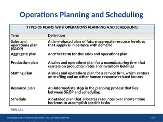
Operations Planning and Scheduling
TYPES OF PLANS WITH OPERATIONS PLANNING AND SCHEDULING
Term Definition
Sales and
operations plan
(S&OP)
A time-phased plan of future aggregate resource levels so
that supply is in balance with demand
Aggregate plan Another term for the sales and operations plan
Production plan A sales and operations plan for a manufacturing firm that
centers on production rates and inventory holdings
Staffing plan A sales and operations plan for a service firm, which centers
on staffing and on other human resource-related factors
Resource plan An intermediate step in the planning process that lies
between S&OP and scheduling
Schedule A detailed plan that allocates resources over shorter time
horizons to accomplish specific tasks
Table 10.1
- 4.
Copyright ©2016 PearsonEducation, Inc. All rights reserved. 10-4
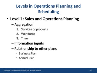
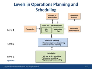
• Level 1: Sales and Operations Planning
– Aggregation
1. Services or products
2. Workforce
3. Time
– Information inputs
– Relationship to other plans
• Business Plan
• Annual Plan
Levels in Operations Planning and
Scheduling
- 5.
Copyright ©2016 PearsonEducation, Inc. All rights reserved. 10-5
Levels in Operations Planning and
Scheduling
Business or
annual plan
• Job and facility scheduling
• Workforce scheduling
• Equipment/jobs scheduling
Scheduling
• Materials requirements planning
• Services resource planning
Resource Planning
Sales
Plan
Operations
Plan
Sales and Operations Plan
Forecasting
Operations
strategy
Constraint
management
Figure 10.2
Level 1
Level 2
Level 3
- 6.
Copyright ©2016 PearsonEducation, Inc. All rights reserved. 10-6
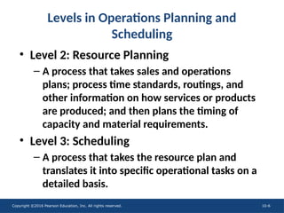
• Level 2: Resource Planning
– A process that takes sales and operations
plans; process time standards, routings, and
other information on how services or products
are produced; and then plans the timing of
capacity and material requirements.
• Level 3: Scheduling
– A process that takes the resource plan and
translates it into specific operational tasks on a
detailed basis.
Levels in Operations Planning and
Scheduling
- 7.
Copyright ©2016 PearsonEducation, Inc. All rights reserved. 10-7
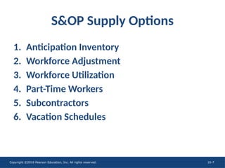
S&OP Supply Options
1. Anticipation Inventory
2. Workforce Adjustment
3. Workforce Utilization
4. Part-Time Workers
5. Subcontractors
6. Vacation Schedules
- 8.
Copyright ©2016 PearsonEducation, Inc. All rights reserved. 10-8
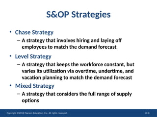
S&OP Strategies
• Chase Strategy
– A strategy that involves hiring and laying off
employees to match the demand forecast
• Level Strategy
– A strategy that keeps the workforce constant, but
varies its utilization via overtime, undertime, and
vacation planning to match the demand forecast
• Mixed Strategy
– A strategy that considers the full range of supply
options
- 9.
Copyright ©2016 PearsonEducation, Inc. All rights reserved. 10-9
S&OP Strategies
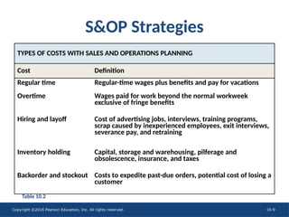
TYPES OF COSTS WITH SALES AND OPERATIONS PLANNING
Cost Definition
Regular time Regular-time wages plus benefits and pay for vacations
Overtime Wages paid for work beyond the normal workweek
exclusive of fringe benefits
Hiring and layoff Cost of advertising jobs, interviews, training programs,
scrap caused by inexperienced employees, exit interviews,
severance pay, and retraining
Inventory holding Capital, storage and warehousing, pilferage and
obsolescence, insurance, and taxes
Backorder and stockout Costs to expedite past-due orders, potential cost of losing a
customer
Table 10.2
- 10.
- 11.
Copyright ©2016 PearsonEducation, Inc. All rights reserved. 10-11
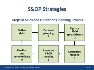
S&OP Strategies
Finalize
and
communicate
6
Executive
S&OP
meeting
5
Consensus
meeting
4
Update
S&OP
spreadsheets
3
Demand
planning
2
Gather
data
1
Steps in Sales and Operations Planning Process
- 12.
- 13.
Copyright ©2016 PearsonEducation, Inc. All rights reserved. 10-13
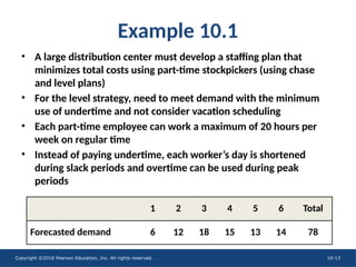
Example 10.1
• A large distribution center must develop a staffing plan that
minimizes total costs using part-time stockpickers (using chase
and level plans)
• For the level strategy, need to meet demand with the minimum
use of undertime and not consider vacation scheduling
• Each part-time employee can work a maximum of 20 hours per
week on regular time
• Instead of paying undertime, each worker’s day is shortened
during slack periods and overtime can be used during peak
periods
1 2 3 4 5 6 Total
Forecasted demand 6 12 18 15 13 14 78
- 14.
Copyright ©2016 PearsonEducation, Inc. All rights reserved. 10-14
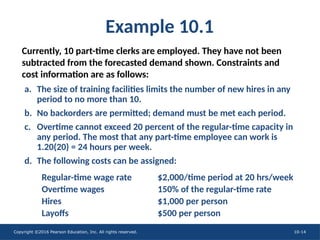
Example 10.1
Currently, 10 part-time clerks are employed. They have not been
subtracted from the forecasted demand shown. Constraints and
cost information are as follows:
a. The size of training facilities limits the number of new hires in any
period to no more than 10.
b. No backorders are permitted; demand must be met each period.
c. Overtime cannot exceed 20 percent of the regular-time capacity in
any period. The most that any part-time employee can work is
1.20(20) = 24 hours per week.
d. The following costs can be assigned:
Regular-time wage rate $2,000/time period at 20 hrs/week
Overtime wages 150% of the regular-time rate
Hires $1,000 per person
Layoffs $500 per person
- 15.
Copyright ©2016 PearsonEducation, Inc. All rights reserved. 10-15
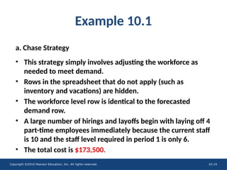
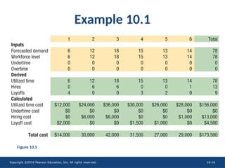
Example 10.1
a. Chase Strategy
• This strategy simply involves adjusting the workforce as
needed to meet demand.
• Rows in the spreadsheet that do not apply (such as
inventory and vacations) are hidden.
• The workforce level row is identical to the forecasted
demand row.
• A large number of hirings and layoffs begin with laying off 4
part-time employees immediately because the current staff
is 10 and the staff level required in period 1 is only 6.
• The total cost is $173,500.
- 16.
- 17.
Copyright ©2016 PearsonEducation, Inc. All rights reserved. 10-17
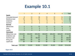
Example 10.1
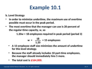
b. Level Strategy
• In order to minimize undertime, the maximum use of overtime
possible must occur in the peak period.
• The most overtime that the manager can use is 20 percent of
the regular-time capacity, w, so
• A 15-employee staff size minimizes the amount of undertime
for this level strategy.
• Because the staff already includes 10 part-time employees,
the manager should immediately hire 5 more.
• The total cost is $164,000.
1.20w = 18 employees required in peak period (period 3)
w = = 15 employees
18
1.20
- 18.
- 19.
Copyright ©2016 PearsonEducation, Inc. All rights reserved. 10-19
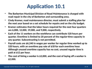
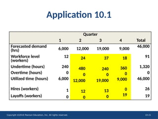
Application 10.1
• The Barberton Municipal Division of Road Maintenance is charged with
road repair in the city of Barberton and surrounding area.
• Cindy Kramer, road maintenance director, must submit a staffing plan for
the next year based on a set schedule for repairs and on the city budget.
• Kramer estimates that the labor hours required for the next four quarters
are 6,000, 12,000, 19,000, and 9,000, respectively.
• Each of the 11 workers on the workforce can contribute 520 hours per
quarter. Overtime is limited to 20 percent of the regular-time capacity in
any quarter. Subcontracting is not permitted.
• Payroll costs are $6,240 in wages per worker for regular time worked up to
520 hours, with an overtime pay rate of $18 for each overtime hour.
Although unused overtime capacity has no cost, unused regular time is
paid at $12 per hour.
• The cost of hiring a worker is $3,000, and the cost of laying off a worker is
$2,000.
- 20.
Copyright ©2016 PearsonEducation, Inc. All rights reserved. 10-20
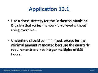
Application 10.1
• Use a chase strategy for the Barberton Municipal
Division that varies the workforce level without
using overtime.
• Undertime should be minimized, except for the
minimal amount mandated because the quarterly
requirements are not integer multiples of 520
hours.
- 21.
Copyright ©2016 PearsonEducation, Inc. All rights reserved. 10-21
Quarter
1 2 3 4 Total
Forecasted demand
(hrs) 6,000 12,000 19,000 9,000
46,000
Workforce level
(workers)
12 91
Undertime (hours) 240 1,320
Overtime (hours) 0 0
Utilized time (hours) 6,000 46,000
Hires (workers) 1 26
Layoffs (workers) 0 19
37
240
0
19,000
13
0
18
360
0
9,000
0
19
Application 10.1
24
480
0
12,000
12
0
- 22.
Copyright ©2016 PearsonEducation, Inc. All rights reserved. 10-22
Application 10.1
What is the total cost of this plan?
Costs per Quarter
1 2 3 4 Total
Utilized time $72,000 $552,000
Undertime 2,880 15,840
Overtime 0 0
Hires 3,000 78,000
Layoffs 0 38,000
Total Cost $683,840
$144,000
5,760
0
36,000
0
$228,000
2,880
0
39,000
0
$108,000
4,320
0
0
38,000
- 23.
Copyright ©2016 PearsonEducation, Inc. All rights reserved. 10-23
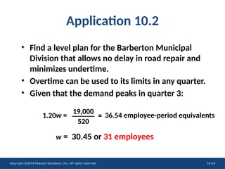
Application 10.2
• Find a level plan for the Barberton Municipal
Division that allows no delay in road repair and
minimizes undertime.
• Overtime can be used to its limits in any quarter.
• Given that the demand peaks in quarter 3:
1.20w =
w = 30.45 or 31 employees
36.54 employee-period equivalents
19,000
520
=
- 24.
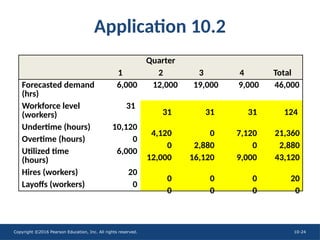
Copyright ©2016 PearsonEducation, Inc. All rights reserved. 10-24
Quarter
1 2 3 4 Total
Forecasted demand
(hrs)
6,000 12,000 19,000 9,000 46,000
Workforce level
(workers)
31
Undertime (hours) 10,120
Overtime (hours) 0
Utilized time
(hours)
6,000
Hires (workers) 20
Layoffs (workers) 0
Application 10.2
31
4,120
0
12,000
0
0
31
0
2,880
16,120
0
0
31
7,120
0
9,000
0
0
124
21,360
2,880
43,120
20
0
- 25.
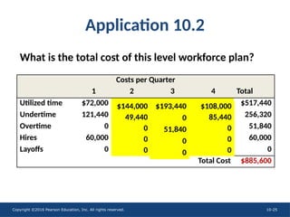
Copyright ©2016 PearsonEducation, Inc. All rights reserved. 10-25
Costs per Quarter
1 2 3 4 Total
Utilized time $72,000 $517,440
Undertime 121,440 256,320
Overtime 0 51,840
Hires 60,000 60,000
Layoffs 0 0
Total Cost $885,600
Application 10.2
What is the total cost of this level workforce plan?
$108,000
85,440
0
0
0
$193,440
0
51,840
0
0
$144,000
49,440
0
0
0
- 26.
Copyright ©2016 PearsonEducation, Inc. All rights reserved. 10-26
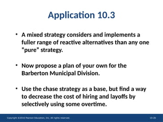
Application 10.3
• A mixed strategy considers and implements a
fuller range of reactive alternatives than any one
“pure” strategy.
• Now propose a plan of your own for the
Barberton Municipal Division.
• Use the chase strategy as a base, but find a way
to decrease the cost of hiring and layoffs by
selectively using some overtime.
- 27.
Copyright ©2016 PearsonEducation, Inc. All rights reserved. 10-27
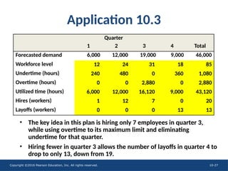
Quarter
1 2 3 4 Total
Forecasted demand 6,000 12,000 19,000 9,000 46,000
Workforce level
Undertime (hours)
Overtime (hours)
Utilized time (hours)
Hires (workers)
Layoffs (workers)
Application 10.3
12
240
0
6,000
1
0
85
1,080
2,880
43,120
20
13
24
480
0
12,000
12
0
31
0
2,880
16,120
7
0
18
360
0
9,000
0
13
• The key idea in this plan is hiring only 7 employees in quarter 3,
while using overtime to its maximum limit and eliminating
undertime for that quarter.
• Hiring fewer in quarter 3 allows the number of layoffs in quarter 4 to
drop to only 13, down from 19.
- 28.
Copyright ©2016 PearsonEducation, Inc. All rights reserved. 10-28
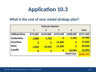
Costs per Quarter
1 2 3 4 Total
Utilized time $72,000 $144,000 $193,440 $108,000 $517,440
Undertime
Overtime
Hires
Layoffs
Total Cost
Application 10.3
What is the cost of your mixed strategy plan?
12,960
51,840
60,000
26,000
$668,240
2,880
0
3,000
0
5,760
0
36,000
0
0
51,840
21,000
0
4,320
0
0
26,000
- 29.
Copyright ©2016 PearsonEducation, Inc. All rights reserved. 10-29
Scheduling
• Scheduling
– The function that takes the operations and
scheduling process from planning to execution.
- 30.
Copyright ©2016 PearsonEducation, Inc. All rights reserved. 10-30
Scheduling
• Job and Facility Scheduling
– Gantt progress chart
– Gantt workstation chart
- 31.
Copyright ©2016 PearsonEducation, Inc. All rights reserved. 10-31
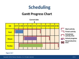
Scheduling
Gantt Progress Chart
Nissan
Ford
Pontiac
Job 4/20 4/22 4/23 4/24 4/25 4/26
4/21
4/17 4/18 4/19
Current date
Start activity
Finish activity
Scheduled
activity time
Actual progress
Nonproductive
time
Figure 10.7
- 32.
Copyright ©2016 PearsonEducation, Inc. All rights reserved. 10-32
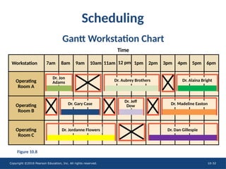
Scheduling
Operating
Room A
Workstation 7am
Operating
Room B
Operating
Room C
12 pm
8am 9am 10am 11am 1pm 2pm 3pm 4pm 5pm 6pm
Time
Dr. Gary Case
Dr. Jeff
Dow Dr. Madeline Easton
Dr. Dan Gillespie
Dr. Jordanne Flowers
Dr. Jon
Adams Dr. Aubrey Brothers Dr. Alaina Bright
Gantt Workstation Chart
Figure 10.8
- 33.
Copyright ©2016 PearsonEducation, Inc. All rights reserved. 10-33
Scheduling
• Workforce Scheduling –
– A type of scheduling that determines when
employees work
• Constraints
– Technical constraints
– Legal and behavioral considerations
– Psychological needs of workers
• Scheduling Options
– Rotating schedule vs Fixed schedule
- 34.
Copyright ©2016 PearsonEducation, Inc. All rights reserved. 10-34
Scheduling
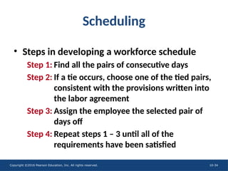
• Steps in developing a workforce schedule
Step 1: Find all the pairs of consecutive days
Step 2: If a tie occurs, choose one of the tied pairs,
consistent with the provisions written into
the labor agreement
Step 3: Assign the employee the selected pair of
days off
Step 4: Repeat steps 1 – 3 until all of the
requirements have been satisfied
- 35.
Copyright ©2016 PearsonEducation, Inc. All rights reserved. 10-35
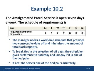
Example 10.2
The Amalgamated Parcel Service is open seven days
a week. The schedule of requirements is:
Day M T W Th F S Su
Required number of
employees 6 4 8 9 10 3 2
• The manager needs a workforce schedule that provides
two consecutive days off and minimizes the amount of
total slack capacity.
• To break ties in the selection of off days, the scheduler
gives preference to Saturday and Sunday if it is one of
the tied pairs.
• If not, she selects one of the tied pairs arbitrarily.
- 36.
Copyright ©2016 PearsonEducation, Inc. All rights reserved. 10-36
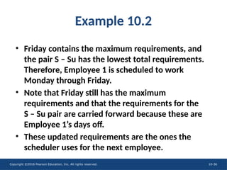
Example 10.2
• Friday contains the maximum requirements, and
the pair S – Su has the lowest total requirements.
Therefore, Employee 1 is scheduled to work
Monday through Friday.
• Note that Friday still has the maximum
requirements and that the requirements for the
S – Su pair are carried forward because these are
Employee 1’s days off.
• These updated requirements are the ones the
scheduler uses for the next employee.
- 37.
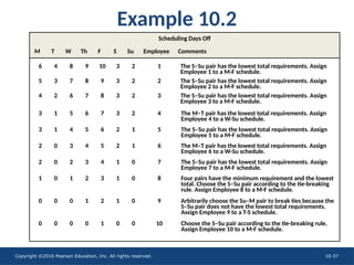
Copyright ©2016 PearsonEducation, Inc. All rights reserved. 10-37
Scheduling Days Off
M T W Th F S Su Employee Comments
6 4 8 9 10 3 2 1 The S–Su pair has the lowest total requirements. Assign
Employee 1 to a M-F schedule.
5 3 7 8 9 3 2 2 The S–Su pair has the lowest total requirements. Assign
Employee 2 to a M-F schedule.
4 2 6 7 8 3 2 3 The S–Su pair has the lowest total requirements. Assign
Employee 3 to a M-F schedule.
3 1 5 6 7 3 2 4 The M–T pair has the lowest total requirements. Assign
Employee 4 to a W-Su schedule.
3 1 4 5 6 2 1 5 The S–Su pair has the lowest total requirements. Assign
Employee 5 to a M-F schedule.
2 0 3 4 5 2 1 6 The M–T pair has the lowest total requirements. Assign
Employee 6 to a W-Su schedule.
2 0 2 3 4 1 0 7 The S–Su pair has the lowest total requirements. Assign
Employee 7 to a M-F schedule.
1 0 1 2 3 1 0 8 Four pairs have the minimum requirement and the lowest
total. Choose the S–Su pair according to the tie-breaking
rule. Assign Employee 8 to a M-F schedule.
0 0 0 1 2 1 0 9 Arbitrarily choose the Su–M pair to break ties because the
S–Su pair does not have the lowest total requirements.
Assign Employee 9 to a T-S schedule.
0 0 0 0 1 0 0 10 Choose the S–Su pair according to the tie-breaking rule.
Assign Employee 10 to a M-F schedule.
Example 10.2
The S–Su pair has the lowest total requirements. Assign
Employee 1 to a M-F schedule.
The S–Su pair has the lowest total requirements. Assign
Employee 2 to a M-F schedule.
The S–Su pair has the lowest total requirements. Assign
Employee 3 to a M-F schedule.
6 4 8 9 10 3 2 1
5 3 7 8 9 3 2 2
4 2 6 7 8 3 2 3
3 1 5 6 7 3 2 4 The M–T pair has the lowest total requirements. Assign
Employee 4 to a W-Su schedule.
3 1 4 5 6 2 1 5 The S–Su pair has the lowest total requirements. Assign
Employee 5 to a M-F schedule.
2 0 3 4 5 2 1 6 The M–T pair has the lowest total requirements. Assign
Employee 6 to a W-Su schedule.
2 0 2 3 4 1 0 7 The S–Su pair has the lowest total requirements. Assign
Employee 7 to a M-F schedule.
1 0 1 2 3 1 0 8 Four pairs have the minimum requirement and the lowest
total. Choose the S–Su pair according to the tie-breaking
rule. Assign Employee 8 to a M-F schedule.
0 0 0 1 2 1 0 9 Arbitrarily choose the Su–M pair to break ties because the
S–Su pair does not have the lowest total requirements.
Assign Employee 9 to a T-S schedule.
0 0 0 0 1 0 0 10 Choose the S–Su pair according to the tie-breaking rule.
Assign Employee 10 to a M-F schedule.
- 38.
Copyright ©2016 PearsonEducation, Inc. All rights reserved. 10-38
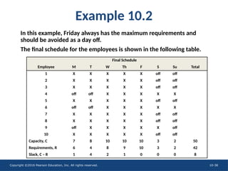
Example 10.2
Final Schedule
Employee M T W Th F S Su Total
1 X X X X X off off
2 X X X X X off off
3 X X X X X off off
4 off off X X X X X
5 X X X X X off off
6 off off X X X X X
7 X X X X X off off
8 X X X X X off off
9 off X X X X X off
10 X X X X X off off
Capacity, C 7 8 10 10 10 3 2 50
Requirements, R 6 4 8 9 10 3 2 42
Slack, C – R 1 4 2 1 0 0 0 8
In this example, Friday always has the maximum requirements and
should be avoided as a day off.
The final schedule for the employees is shown in the following table.
- 39.
Copyright ©2016 PearsonEducation, Inc. All rights reserved. 10-39
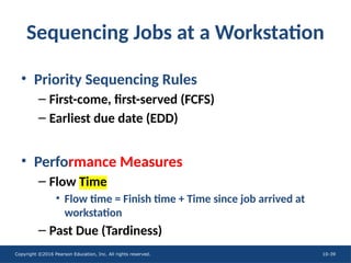
Sequencing Jobs at a Workstation
• Priority Sequencing Rules
– First-come, first-served (FCFS)
– Earliest due date (EDD)
• Performance Measures
– Flow Time
• Flow time = Finish time + Time since job arrived at
workstation
– Past Due (Tardiness)
- 40.
Copyright ©2016 PearsonEducation, Inc. All rights reserved. 10-40
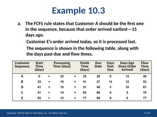
Example 10.3
27 14 12 53
41 + 10 = 51 48 3 10 61
51 + 14 = 65 68 0 5 70
65 + 12 = 77 80 0 0 77
15 40
+ 25 = 25 29 0
0
25 + 16 = 41
Customer
Sequence
Start
Time
(days)
Processing
Time (days)
Finish
Time
(days)
Due
Date
Days
Past
Due
Days Ago
Since Order
Arrived
Flow
Time
(days)
A
B
D
C
E
a. The FCFS rule states that Customer A should be the first one
in the sequence, because that order arrived earliest—15
days ago.
Customer E’s order arrived today, so it is processed last.
The sequence is shown in the following table, along with
the days past due and flow times.
- 41.
Copyright ©2016 PearsonEducation, Inc. All rights reserved. 10-41
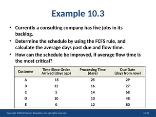
Example 10.3
• Currently a consulting company has five jobs in its
backlog.
• Determine the schedule by using the FCFS rule, and
calculate the average days past due and flow time.
• How can the schedule be improved, if average flow time is
the most critical?
Customer Time Since Order
Arrived (days ago)
Processing Time
(days)
Due Date
(days from now)
A 15 25 29
B 12 16 27
C 5 14 68
D 10 10 48
E 0 12 80
- 42.
Copyright ©2016 PearsonEducation, Inc. All rights reserved. 10-42
Example 10.3
The finish time for a job is its start time plus the processing time. Its
finish time becomes the start time for the next job in the sequence,
assuming that the next job is available for immediate processing. The
days past due for a job is zero (0) if its due date is equal to or exceeds
the finish time. Otherwise it equals the shortfall. The flow time for
each job equals its finish time plus the number of days ago since the
order first arrived at the workstation. The days past due and average
flow time performance measures for the FCFS schedule are
Average days past due =
Average flow time =
= 3.4 days
= 60.2 days
0 + 14 + 3 + 0 + 0
5
40 + 53 + 61 + 70 + 77
5
- 43.
Copyright ©2016 PearsonEducation, Inc. All rights reserved. 10-43
Example 10.3
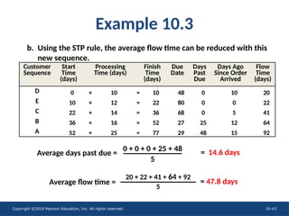
b. Using the STP rule, the average flow time can be reduced with this
new sequence.
0 + 10 = 10
Customer
Sequence
Start
Time
(days)
Processing
Time (days)
Finish
Time
(days)
Due
Date
Days
Past
Due
Days Ago
Since Order
Arrived
Flow
Time
(days)
D
E
C
B
A
Average days past due =
Average flow time =
= 14.6 days
= 47.8 days
0 + 0 + 0 + 25 + 48
5
20 + 22 + 41 + 64 + 92
5
22 + 14 = 36 68 0 5 41
36 + 16 = 52 27 25 12 64
52 + 25 = 77 29 48 15 92
48 0 10 20
10 + 12 = 22 80 0 0 22
- 44.
Copyright ©2016 PearsonEducation, Inc. All rights reserved. 10-44
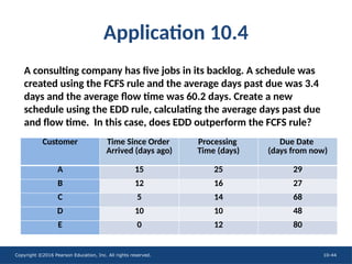
A consulting company has five jobs in its backlog. A schedule was
created using the FCFS rule and the average days past due was 3.4
days and the average flow time was 60.2 days. Create a new
schedule using the EDD rule, calculating the average days past due
and flow time. In this case, does EDD outperform the FCFS rule?
Application 10.4
Customer Time Since Order
Arrived (days ago)
Processing
Time (days)
Due Date
(days from now)
A 15 25 29
B 12 16 27
C 5 14 68
D 10 10 48
E 0 12 80
- 45.
Copyright ©2016 PearsonEducation, Inc. All rights reserved. 10-45
Customer
Sequence
Start
Time
(days)
Processing
Time (days)
Finish
Time
(days)
Due
Date
Days
Past
Due
Days Ago
Since Order
Arrived
Flow
Time
(days)
B
A
D
C
E
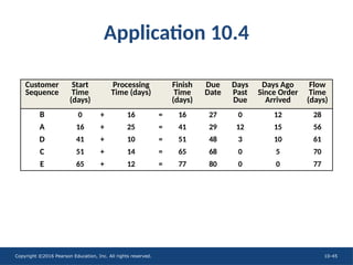
Application 10.4
0 + 16 = 16
41 + 10 = 51 48 3 10 61
51 + 14 = 65 68 0 5 70
65 + 12 = 77 80 0 0 77
27 0 12 28
16 + 25 = 41 29 12 15 56
- 46.
Copyright ©2016 PearsonEducation, Inc. All rights reserved. 10-46
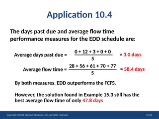
Application 10.4
The days past due and average flow time
performance measures for the EDD schedule are:
By both measures, EDD outperforms the FCFS.
However, the solution found in Example 15.3 still has the
best average flow time of only 47.8 days
Average days past due =
Average flow time =
= 3.0 days
= 58.4 days
0 + 12 + 3 + 0 + 0
5
28 + 56 + 61 + 70 + 77
5
- 47.
Copyright ©2016 PearsonEducation, Inc. All rights reserved. 10-47
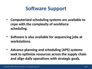
Software Support
• Computerized scheduling systems are available to
cope with the complexity of workforce
scheduling.
• Software is also available for sequencing jobs at
workstations.
• Advance planning and scheduling (APS) systems
seek to optimize resources across the supply chain
and align daily operations with strategic goals.
- 48.
Copyright ©2016 PearsonEducation, Inc. All rights reserved. 10-48
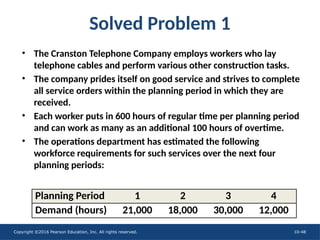
Solved Problem 1
• The Cranston Telephone Company employs workers who lay
telephone cables and perform various other construction tasks.
• The company prides itself on good service and strives to complete
all service orders within the planning period in which they are
received.
• Each worker puts in 600 hours of regular time per planning period
and can work as many as an additional 100 hours of overtime.
• The operations department has estimated the following
workforce requirements for such services over the next four
planning periods:
Planning Period 1 2 3 4
Demand (hours) 21,000 18,000 30,000 12,000
- 49.
Copyright ©2016 PearsonEducation, Inc. All rights reserved. 10-49
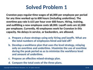
Solved Problem 1
Cranston pays regular-time wages of $6,000 per employee per period
for any time worked up to 600 hours (including undertime). The
overtime pay rate is $15 per hour over 600 hours. Hiring, training,
and outfitting a new employee costs $8,000. Layoff costs are $2,000
per employee. Currently, 40 employees work for Cranston in this
capacity. No delays in service, or backorders, are allowed.
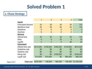
a. Prepare a chase strategy using only hiring and layoffs. What are
the total numbers of employees hired and laid off?
b. Develop a workforce plan that uses the level strategy, relaying
only on overtime and undertime. Maximize the use of overtime
during the peak period so as to minimize the workforce level
and amount of undertime.
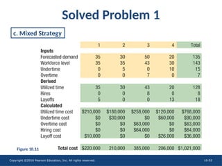
c. Propose an effective mixed-strategy plan.
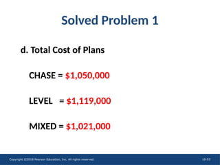
d. Compare the total costs of the three plans.
- 50.
- 51.
- 52.
- 53.
Copyright ©2016 PearsonEducation, Inc. All rights reserved. 10-53
Solved Problem 1
d. Total Cost of Plans
CHASE = $1,050,000
LEVEL = $1,119,000
MIXED = $1,021,000
- 54.
Copyright ©2016 PearsonEducation, Inc. All rights reserved. 10-54
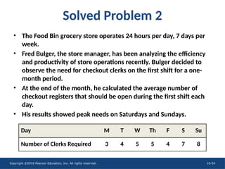
Solved Problem 2
• The Food Bin grocery store operates 24 hours per day, 7 days per
week.
• Fred Bulger, the store manager, has been analyzing the efficiency
and productivity of store operations recently. Bulger decided to
observe the need for checkout clerks on the first shift for a one-
month period.
• At the end of the month, he calculated the average number of
checkout registers that should be open during the first shift each
day.
• His results showed peak needs on Saturdays and Sundays.
Day M T W Th F S Su
Number of Clerks Required 3 4 5 5 4 7 8
- 55.
Copyright ©2016 PearsonEducation, Inc. All rights reserved. 10-55
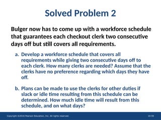
Solved Problem 2
Bulger now has to come up with a workforce schedule
that guarantees each checkout clerk two consecutive
days off but still covers all requirements.
a. Develop a workforce schedule that covers all
requirements while giving two consecutive days off to
each clerk. How many clerks are needed? Assume that the
clerks have no preference regarding which days they have
off.
b. Plans can be made to use the clerks for other duties if
slack or idle time resulting from this schedule can be
determined. How much idle time will result from this
schedule, and on what days?
- 56.
Copyright ©2016 PearsonEducation, Inc. All rights reserved. 10-56
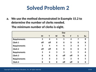
Solved Problem 2
a. We use the method demonstrated in Example 15.2 to
determine the number of clerks needed.
The minimum number of clerks is eight.
3 4 5 5 4 7 8
off off X X X X X
3 4 4 4 3 6 7
off off X X X X X
Day
M T W Th F S Su
Requirements
Clerk 1
Requirements
Clerk 2
Requirements
Clerk 3
Requirements
Clerk 4
3 4 3 3 2 5 6
X X X off off X X
2 3 2 3 2 4 5
X X X off off X X
- 57.
Copyright ©2016 PearsonEducation, Inc. All rights reserved. 10-57
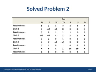
Solved Problem 2
1 2 1 3 2 3 4
X off off X X X X
0 2 1 2 1 2 3
off off X X X X X
0 2 0 1 0 1 2
X X off off X X X
0 1 0 1 0 0 1
X X X X off off X
0 0 0 0 0 0 0
Day
M T W Th F S Su
Requirements
Clerk 5
Requirements
Clerk 6
Requirements
Clerk 7
Requirements
Clerk 8
Requirements
- 58.
Copyright ©2016 PearsonEducation, Inc. All rights reserved. 10-58
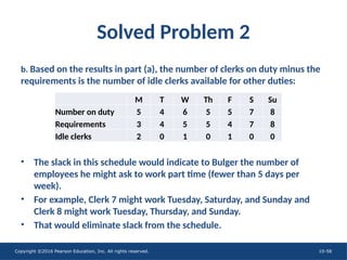
Solved Problem 2
b. Based on the results in part (a), the number of clerks on duty minus the
requirements is the number of idle clerks available for other duties:
• The slack in this schedule would indicate to Bulger the number of
employees he might ask to work part time (fewer than 5 days per
week).
• For example, Clerk 7 might work Tuesday, Saturday, and Sunday and
Clerk 8 might work Tuesday, Thursday, and Sunday.
• That would eliminate slack from the schedule.
M T W Th F S Su
Number on duty 5 4 6 5 5 7 8
Requirements 3 4 5 5 4 7 8
Idle clerks 2 0 1 0 1 0 0