Download as PDF, PPTX
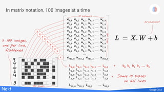
![Softmax, on a batch of images
Predictions Images Weights Biases
Y[100, 10] X[100, 784] W[784,10] b[10]
matrix multiply
broadcast
on all lines
applied line
by line
tensor shapes in [ ]](https://image.slidesharecdn.com/3laqqo2lr7uafek8if1p-signature-a67b506a92064307cfedba3a781e15cbc2f0c6a86a8ed39575da2d26819992de-poli-171121170308/85/Lucio-Floretta-TensorFlow-and-Deep-Learning-without-a-PhD-Codemotion-Milan-2017-5-320.jpg)
![Now in TensorFlow (Python)
Y = tf.nn.softmax(tf.matmul(X, W) + b)
tensor shapes: X[100, 784] W[748,10] b[10]
matrix multiply
broadcast
on all lines](https://image.slidesharecdn.com/3laqqo2lr7uafek8if1p-signature-a67b506a92064307cfedba3a781e15cbc2f0c6a86a8ed39575da2d26819992de-poli-171121170308/85/Lucio-Floretta-TensorFlow-and-Deep-Learning-without-a-PhD-Codemotion-Milan-2017-6-320.jpg)
![TensorFlow - initialisation
import tensorflow as tf
X = tf.placeholder(tf.float32, [None, 28, 28, 1])
W = tf.Variable(tf.zeros([784, 10]))
b = tf.Variable(tf.zeros([10]))
init = tf.initialize_all_variables()
this will become the batch size
28 x 28 grayscale images
Training = computing variables W and b](https://image.slidesharecdn.com/3laqqo2lr7uafek8if1p-signature-a67b506a92064307cfedba3a781e15cbc2f0c6a86a8ed39575da2d26819992de-poli-171121170308/85/Lucio-Floretta-TensorFlow-and-Deep-Learning-without-a-PhD-Codemotion-Milan-2017-10-320.jpg)
![# model
Y = tf.nn.softmax(tf.matmul(tf.reshape(X, [-1, 784]), W) + b)
# placeholder for correct answers
Y_ = tf.placeholder(tf.float32, [None, 10])
# loss function
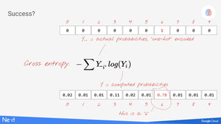
cross_entropy = -tf.reduce_sum(Y_ * tf.log(Y))
TensorFlow - success metrics
“one-hot” encoded
flattening images](https://image.slidesharecdn.com/3laqqo2lr7uafek8if1p-signature-a67b506a92064307cfedba3a781e15cbc2f0c6a86a8ed39575da2d26819992de-poli-171121170308/85/Lucio-Floretta-TensorFlow-and-Deep-Learning-without-a-PhD-Codemotion-Milan-2017-11-320.jpg)
![import tensorflow as tf
X = tf.placeholder(tf.float32, [None, 28, 28, 1])
W = tf.Variable(tf.zeros([784, 10]))
b = tf.Variable(tf.zeros([10]))
init = tf.initialize_all_variables()
# model
Y=tf.nn.softmax(tf.matmul(tf.reshape(X,[-1, 784]), W) + b)
# placeholder for correct answers
Y_ = tf.placeholder(tf.float32, [None, 10])
# loss function
cross_entropy = -tf.reduce_sum(Y_ * tf.log(Y))
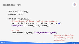
TensorFlow - full python code
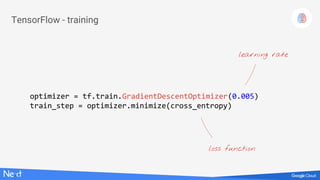
optimizer = tf.train.GradientDescentOptimizer(0.005)
train_step = optimizer.minimize(cross_entropy)
sess = tf.Session()
sess.run(init)
for i in range(10000):
# load batch of images and correct answers
batch_X, batch_Y = mnist.train.next_batch(100)
train_data={X: batch_X, Y_: batch_Y}
# train
sess.run(train_step, feed_dict=train_data)
initialisation
model
success metrics
training step
Run](https://image.slidesharecdn.com/3laqqo2lr7uafek8if1p-signature-a67b506a92064307cfedba3a781e15cbc2f0c6a86a8ed39575da2d26819992de-poli-171121170308/85/Lucio-Floretta-TensorFlow-and-Deep-Learning-without-a-PhD-Codemotion-Milan-2017-14-320.jpg)


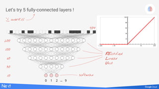
![TensorFlow - initialisation
K = 200
L = 100
M = 60
N = 30
W1 = tf.Variable(tf.truncated_normal([28*28, K] ,stddev=0.1))
B1 = tf.Variable(tf.zeros([K]))
W2 = tf.Variable(tf.truncated_normal([K, L], stddev=0.1))
B2 = tf.Variable(tf.zeros([L]))
W3 = tf.Variable(tf.truncated_normal([L, M], stddev=0.1))
B3 = tf.Variable(tf.zeros([M]))
W4 = tf.Variable(tf.truncated_normal([M, N], stddev=0.1))
B4 = tf.Variable(tf.zeros([N]))
W5 = tf.Variable(tf.truncated_normal([N, 10], stddev=0.1))
B5 = tf.Variable(tf.zeros([10]))
weights initialised
with random values](https://image.slidesharecdn.com/3laqqo2lr7uafek8if1p-signature-a67b506a92064307cfedba3a781e15cbc2f0c6a86a8ed39575da2d26819992de-poli-171121170308/85/Lucio-Floretta-TensorFlow-and-Deep-Learning-without-a-PhD-Codemotion-Milan-2017-18-320.jpg)
![TensorFlow - the model
X = tf.reshape(X, [-1, 28*28])
Y1 = tf.nn.relu(tf.matmul(X, W1) + B1)
Y2 = tf.nn.relu(tf.matmul(Y1, W2) + B2)
Y3 = tf.nn.relu(tf.matmul(Y2, W3) + B3)
Y4 = tf.nn.relu(tf.matmul(Y3, W4) + B4)
Y = tf.nn.softmax(tf.matmul(Y4, W5) + B5)
weights and biases](https://image.slidesharecdn.com/3laqqo2lr7uafek8if1p-signature-a67b506a92064307cfedba3a781e15cbc2f0c6a86a8ed39575da2d26819992de-poli-171121170308/85/Lucio-Floretta-TensorFlow-and-Deep-Learning-without-a-PhD-Codemotion-Milan-2017-19-320.jpg)


![W1
[4, 4, 3]
W2
[4, 4, 3]
+padding
W[4, 4, 3, 2]
filter
size
input
channels
output
channels
stride
convolutional
subsampling
convolutional
subsampling
convolutional
subsampling
Convolutional layer](https://image.slidesharecdn.com/3laqqo2lr7uafek8if1p-signature-a67b506a92064307cfedba3a781e15cbc2f0c6a86a8ed39575da2d26819992de-poli-171121170308/85/Lucio-Floretta-TensorFlow-and-Deep-Learning-without-a-PhD-Codemotion-Milan-2017-29-320.jpg)

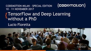
![Convolutional neural network
convolutional layer, 4 channels
W1[5, 5, 1, 4] stride 1
convolutional layer, 8 channels
W2[4, 4, 4, 8] stride 2
convolutional layer, 12 channels
W3[4, 4, 8, 12] stride 2
28x28x1
28x28x4
14x14x8
200
7x7x12
10
fully connected layer W4[7x7x12, 200]
softmax readout layer W5[200, 10]
+ biases on
all layers](https://image.slidesharecdn.com/3laqqo2lr7uafek8if1p-signature-a67b506a92064307cfedba3a781e15cbc2f0c6a86a8ed39575da2d26819992de-poli-171121170308/85/Lucio-Floretta-TensorFlow-and-Deep-Learning-without-a-PhD-Codemotion-Milan-2017-31-320.jpg)
![Tensorflow - initialisation
W1 = tf.Variable(tf.truncated_normal([5, 5, 1, 4] ,stddev=0.1))
B1 = tf.Variable(tf.ones([4])/10)
W2 = tf.Variable(tf.truncated_normal([5, 5, 4, 8] ,stddev=0.1))
B2 = tf.Variable(tf.ones([8])/10)
W3 = tf.Variable(tf.truncated_normal([4, 4, 8, 12] ,stddev=0.1))
B3 = tf.Variable(tf.ones([12])/10)
W4 = tf.Variable(tf.truncated_normal([7*7*12, 200] ,stddev=0.1))
B4 = tf.Variable(tf.ones([200])/10)
W5 = tf.Variable(tf.truncated_normal([200, 10] ,stddev=0.1))
B5 = tf.Variable(tf.zeros([10])/10)
filter
size
input
channels
output
channels
weights initialised
with random values](https://image.slidesharecdn.com/3laqqo2lr7uafek8if1p-signature-a67b506a92064307cfedba3a781e15cbc2f0c6a86a8ed39575da2d26819992de-poli-171121170308/85/Lucio-Floretta-TensorFlow-and-Deep-Learning-without-a-PhD-Codemotion-Milan-2017-32-320.jpg)
![Tensorflow - the model
Y1 = tf.nn.relu(tf.nn.conv2d(X, W1, strides=[1, 1, 1, 1], padding='SAME') + B1)
Y2 = tf.nn.relu(tf.nn.conv2d(Y1, W2, strides=[1, 2, 2, 1], padding='SAME') + B2)
Y3 = tf.nn.relu(tf.nn.conv2d(Y2, W3, strides=[1, 2, 2, 1], padding='SAME') + B3)
YY = tf.reshape(Y3, shape=[-1, 7 * 7 * 12])
Y4 = tf.nn.relu(tf.matmul(YY, W4) + B4)
Y = tf.nn.softmax(tf.matmul(Y4, W5) + B5)
weights biasesstride
flatten all values for
fully connected layer
input image batch
X[100, 28, 28, 1]
Y3 [100, 7, 7, 12]
YY [100, 7x7x12]](https://image.slidesharecdn.com/3laqqo2lr7uafek8if1p-signature-a67b506a92064307cfedba3a781e15cbc2f0c6a86a8ed39575da2d26819992de-poli-171121170308/85/Lucio-Floretta-TensorFlow-and-Deep-Learning-without-a-PhD-Codemotion-Milan-2017-33-320.jpg)

![Bigger convolutional network + dropout
convolutional layer, 12 channels
W2[5, 5, 6, 12] stride 2
convolutional layer, 12 channels
W2[5, 5, 6, 12] stride 2
convolutional layer, 6 channels
W1[6, 6, 1, 6] stride 1
convolutional layer, 24 channels
W3[4, 4, 12, 24] stride 2
convolutional layer, 24 channels
W3[4, 4, 12, 24] stride 2
convolutional layer, 6 channels
W1[6, 6, 1, 6] stride 1
28x28x1
28x28x6
14x14x12
200
7x7x24
10
fully connected layer W4[7x7x24, 200]
softmax readout layer W5[200, 10]
+ biases on
all layers
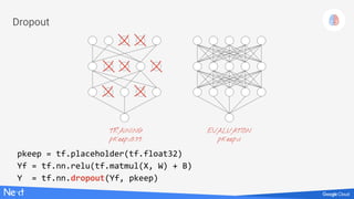
+DROPOUT
p=0.75](https://image.slidesharecdn.com/3laqqo2lr7uafek8if1p-signature-a67b506a92064307cfedba3a781e15cbc2f0c6a86a8ed39575da2d26819992de-poli-171121170308/85/Lucio-Floretta-TensorFlow-and-Deep-Learning-without-a-PhD-Codemotion-Milan-2017-36-320.jpg)
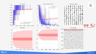
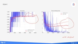


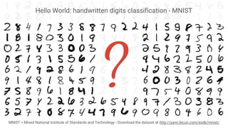
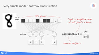
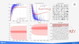
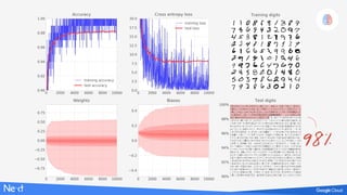
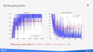
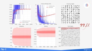
The document discusses implementing deep learning using TensorFlow, focusing on classifying handwritten digits from the MNIST dataset. It provides a detailed breakdown of the architecture, initialization, and training processes, including the use of layers, activation functions, and dropout techniques. The document also highlights various strategies to optimize performance, such as adjusting learning rates and employing convolutional layers.