Algorithms

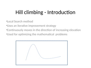
1. Hill climbing - Introduction
•Local Search method
•Uses an iterative improvement strategy
•Continuously moves in the direction of increasing elevation
•Used for optimizing the mathematical problems

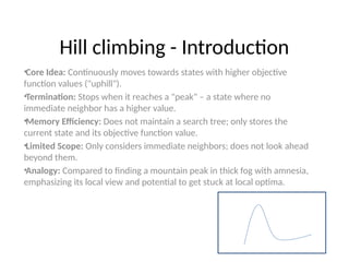
2. Hill climbing - Introduction
•Core Idea: Continuously moves towards states with higher objective
function values ("uphill").
•Termination: Stops when it reaches a "peak" – a state where no
immediate neighbor has a higher value.
•Memory Efficiency: Does not maintain a search tree; only stores the
current state and its objective function value.
•Limited Scope: Only considers immediate neighbors; does not look ahead
beyond them.
•Analogy: Compared to finding a mountain peak in thick fog with amnesia,
emphasizing its local view and potential to get stuck at local optima.

3. Steps in Hill Climbing
• Applied to a single point – the current point(or
state) – in the search space.
• At each iteration , a new point x’ is selected by
performing a small displacement in the current
point x .
• Depending on the representation used for x,
this can be implemented by simply adding a
small random number ,DELTA X, to the current
value of x:x’=x+deltaX.

4. • If that new point provides a better value for
the evaluation function , then the new point
become the current point .
• Else , some other displacement is promoted in
the current point ( a new neighbour is chosen)
and tested against its previous value.

5. Stopping criteria – Hill Climbing
• No Further improvement can be made
• A fixed number of iteration have been
performed
• A goal point is attained

6. Algorithm –hill climbing
Procedure [x] =hill-climbing (max_it,g)
Initialize x
eval(x)
T 1
While t< max_it & x!=g & no_improvement do ,
x’  perturb(x)
eval(x’)
if eval(x’) is better than eval(x),
then x x’
end if
t  t+1
end while
end procedure

7. Different regions –state space
• Local maxima and global maxima
Local maxima
Global Maxima

8. Different regions –state space
• Plateua /flat local maximum
Flat Local Maximum

9. Different regions –state space
• Ridge

10. Iterated –Hill climbing

11. Iterated –Hill climbing
Starts from number of random points
Procedure [best] –IHC(n_start,max_it,g)
Initialize best
T1  1
While t1 <n_start & best !=g do,
Initialize x
eval (x)
x hill –climbing (max_it,g) // Algorithm 1
T1 t1+1
If x is better that best,
then best  x
End if
End while
End procedure

12. Stochastic –hill climbing
Accepts X’ With some probability
Procedure [x] =Stochastic hill-climbing (max_it,g)
Initialize x
eval(x)
T 1
While t< max_it & x!=g & no_improvement do ,
x’  perturb(x)
eval(x’)
if random(0,1) < (1/(1+exp[(eval(x)-eval(x’))/T])),
then x x’
end if
t  t+1
end while
end procedure