This document is the preface to Schaum's Outlines Linear Algebra Fourth Edition. It introduces the topics covered in the textbook, which include vectors in Euclidean space, matrix algebra, systems of linear equations, vector spaces, linear mappings, inner product spaces, orthogonality, determinants, diagonalization through eigenvalues and eigenvectors, and canonical forms. The preface describes the organization of the textbook and highlights changes made in the fourth edition such as expanded appendices on additional mathematical concepts.

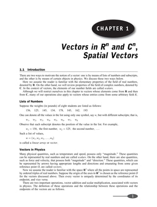
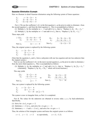
![1.5 Located Vectors, Hyperplanes, Lines, Curves in Rn
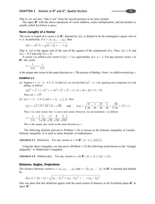
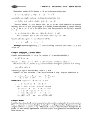
This section distinguishes between an n-tuple PðaiÞ Pða1; a2; . . . ; anÞ viewed as a point in Rn
and an
n-tuple u ¼ ½c1; c2; . . . ; cn viewed as a vector (arrow) from the origin O to the point Cðc1; c2; . . . ; cnÞ.
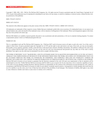
Located Vectors
Any pair of points AðaiÞ and BðbiÞ in Rn
defines the located vector or directed line segment from A to B,
written AB
!
. We identify AB
!
with the vector
u ¼ B A ¼ ½b1 a1; b2 a2; . . . ; bn an
because AB
!
and u have the same magnitude and direction. This is pictured in Fig. 1-2(b) for the
points Aða1; a2; a3Þ and Bðb1; b2; b3Þ in R3
and the vector u ¼ B A which has the endpoint
Pðb1 a1, b2 a2, b3 a3Þ.
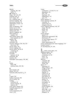
Hyperplanes
A hyperplane H in Rn
is the set of points ðx1; x2; . . . ; xnÞ that satisfy a linear equation
a1x1 þ a2x2 þ þ anxn ¼ b
where the vector u ¼ ½a1; a2; . . . ; an of coefficients is not zero. Thus a hyperplane H in R2
is a line, and a
hyperplane H in R3
is a plane. We show below, as pictured in Fig. 1-3(a) for R3
, that u is orthogonal to
any directed line segment PQ
!
, where Pð piÞ and QðqiÞ are points in H: [For this reason, we say that u is
normal to H and that H is normal to u:]
Because Pð piÞ and QðqiÞ belong to H; they satisfy the above hyperplane equation—that is,
a1 p1 þ a2 p2 þ þ an pn ¼ b and a1q1 þ a2q2 þ þ anqn ¼ b
v ¼ PQ
!
¼ Q P ¼ ½q1 p1; q2 p2; . . . ; qn pn
Let
Then
u v ¼ a1ðq1 p1Þ þ a2ðq2 p2Þ þ þ anðqn pnÞ
¼ ða1q1 þ a2q2 þ þ anqnÞ ða1 p1 þ a2 p2 þ þ an pnÞ ¼ b b ¼ 0
Thus v ¼ PQ
!
is orthogonal to u; as claimed.
Figure 1-3
CHAPTER 1 Vectors in Rn
and Cn
, Spatial Vectors 7](https://image.slidesharecdn.com/linearalgebra4thedition-231030053714-df1faee2/85/Linear_Algebra-_4th_Edition-pdf-14-320.jpg)
![which is tangent to the curve. Normalizing VðtÞ yields
TðtÞ ¼
VðtÞ
kVðtÞk
Thus, TðtÞ is the unit tangent vector to the curve. (Unit vectors with geometrical significance are often
presented in bold type.)
EXAMPLE 1.7 Consider the curve FðtÞ ¼ ½sin t; cos t; t in R3
. Taking the derivative of FðtÞ [or each component of
FðtÞ] yields
VðtÞ ¼ ½cos t; sin t; 1
which is a vector tangent to the curve. We normalize VðtÞ. First we obtain
kVðtÞk2
¼ cos2
t þ sin2
t þ 1 ¼ 1 þ 1 ¼ 2
Then the unit tangent vection TðtÞ to the curve follows:
TðtÞ ¼
VðtÞ
kVðtÞk
¼
cos t
ffiffiffi
2
p ;
sin t
ffiffiffi
2
p ;
1
ffiffiffi
2
p
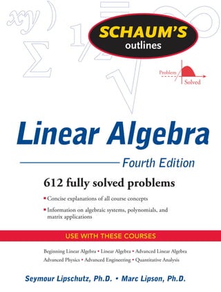
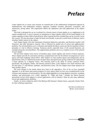
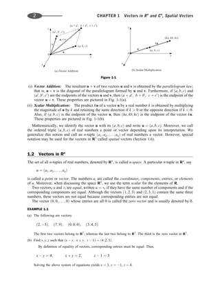
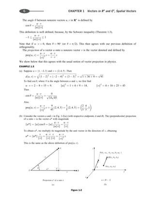
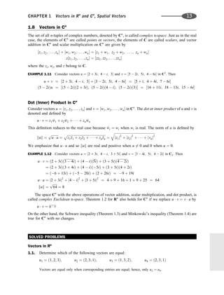
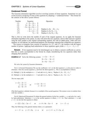
1.6 Vectors in R3
(Spatial Vectors), ijk Notation
Vectors in R3
, called spatial vectors, appear in many applications, especially in physics. In fact, a special
notation is frequently used for such vectors as follows:
i ¼ ½1; 0; 0 denotes the unit vector in the x direction:
j ¼ ½0; 1; 0 denotes the unit vector in the y direction:
k ¼ ½0; 0; 1 denotes the unit vector in the z direction:
Then any vector u ¼ ½a; b; c in R3
can be expressed uniquely in the form
u ¼ ½a; b; c ¼ ai þ bj þ cj
Because the vectors i; j; k are unit vectors and are mutually orthogonal, we obtain the following dot
products:
i i ¼ 1; j j ¼ 1; k k ¼ 1 and i j ¼ 0; i k ¼ 0; j k ¼ 0
Furthermore, the vector operations discussed above may be expressed in the ijk notation as follows.
Suppose
u ¼ a1i þ a2j þ a3k and v ¼ b1i þ b2j þ b3k
Then
u þ v ¼ ða1 þ b1Þi þ ða2 þ b2Þj þ ða3 þ b3Þk and cu ¼ ca1i þ ca2j þ ca3k
where c is a scalar. Also,
u v ¼ a1b1 þ a2b2 þ a3b3 and kuk ¼
ffiffiffiffiffiffiffiffiffi
u u
p
¼ a2
1 þ a2
2 þ a2
3
EXAMPLE 1.8 Suppose u ¼ 3i þ 5j 2k and v ¼ 4i 8j þ 7k.
(a) To find u þ v, add corresponding components, obtaining u þ v ¼ 7i 3j þ 5k
(b) To find 3u 2v, first multiply by the scalars and then add:
3u 2v ¼ ð9i þ 13j 6kÞ þ ð8i þ 16j 14kÞ ¼ i þ 29j 20k
CHAPTER 1 Vectors in Rn
and Cn
, Spatial Vectors 9](https://image.slidesharecdn.com/linearalgebra4thedition-231030053714-df1faee2/85/Linear_Algebra-_4th_Edition-pdf-16-320.jpg)
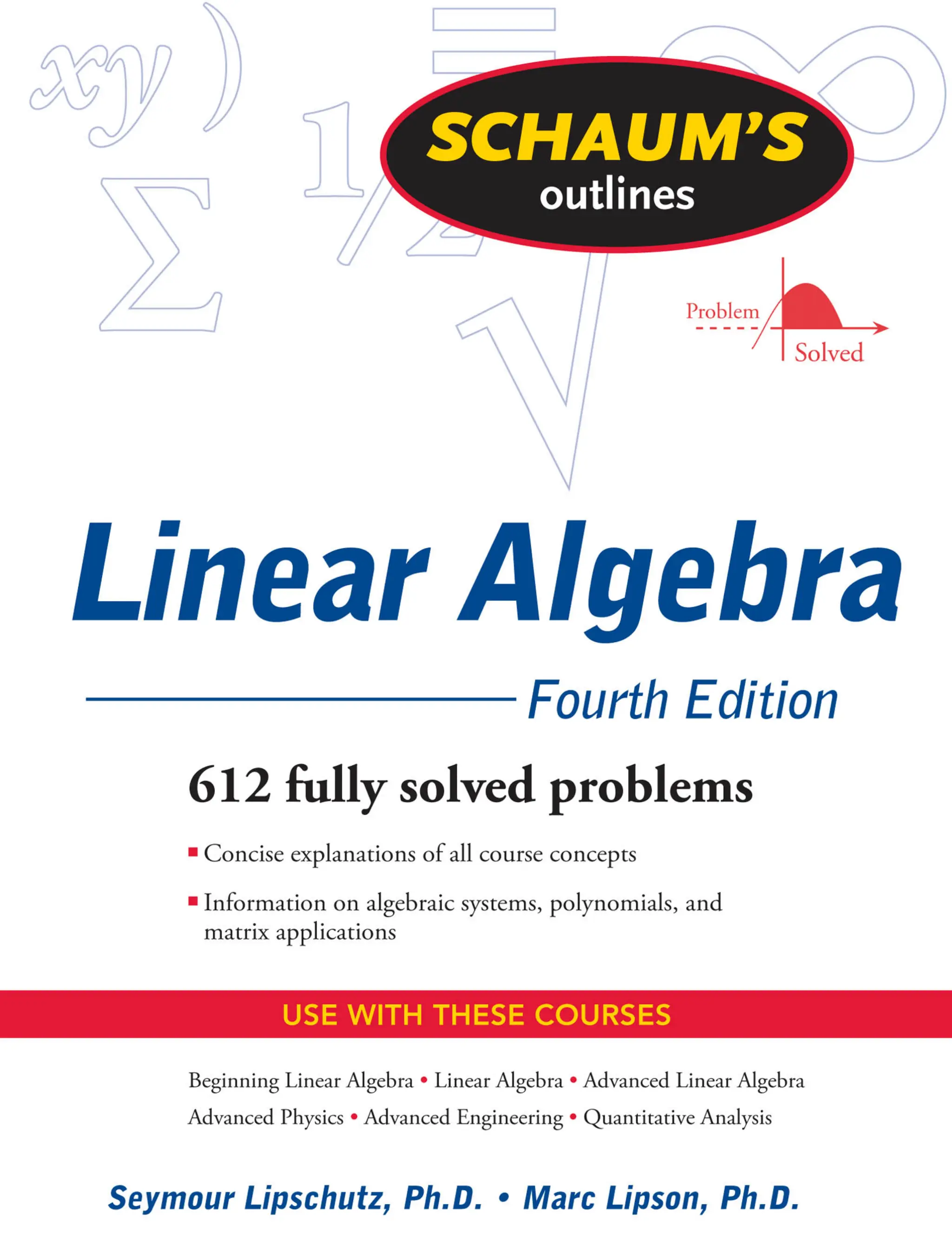
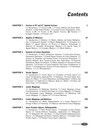
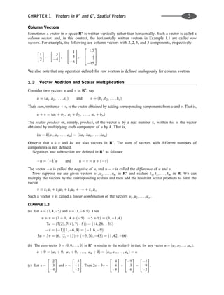
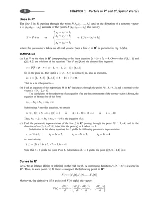
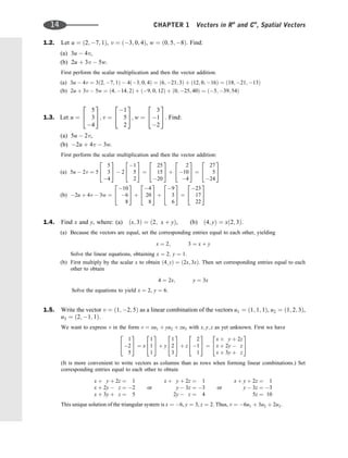
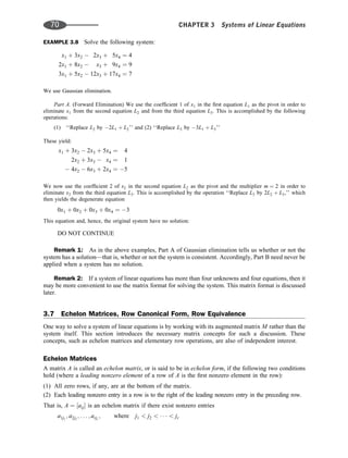
![THEOREM 1.5: Let u; v; w be vectors in R3
.
(a) The vector u v is orthogonal to both u and v.
(b) The absolute value of the ‘‘triple product’’
u v w
represents the volume of the parallelopiped formed by the vectors u; v, w.
[See Fig. 1-4(a).]
We note that the vectors u; v, u v form a right-handed system, and that the following formula
gives the magnitude of u v:
ku vk ¼ kukkvk sin y
where y is the angle between u and v.
1.7 Complex Numbers
The set of complex numbers is denoted by C. Formally, a complex number is an ordered pair ða; bÞ of
real numbers where equality, addition, and multiplication are defined as follows:
ða; bÞ ¼ ðc; dÞ if and only if a ¼ c and b ¼ d
ða; bÞ þ ðc; dÞ ¼ ða þ c; b þ dÞ
ða; bÞ ðc; dÞ ¼ ðac bd; ad þ bcÞ
We identify the real number a with the complex number ða; 0Þ; that is,
a $ ða; 0Þ
This is possible because the operations of addition and multiplication of real numbers are preserved under
the correspondence; that is,
ða; 0Þ þ ðb; 0Þ ¼ ða þ b; 0Þ and ða; 0Þ ðb; 0Þ ¼ ðab; 0Þ
Thus we view R as a subset of C, and replace ða; 0Þ by a whenever convenient and possible.
We note that the set C of complex numbers with the above operations of addition and multiplication is
a field of numbers, like the set R of real numbers and the set Q of rational numbers.
Figure 1-4
CHAPTER 1 Vectors in Rn
and Cn
, Spatial Vectors 11](https://image.slidesharecdn.com/linearalgebra4thedition-231030053714-df1faee2/85/Linear_Algebra-_4th_Edition-pdf-18-320.jpg)
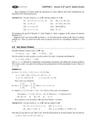
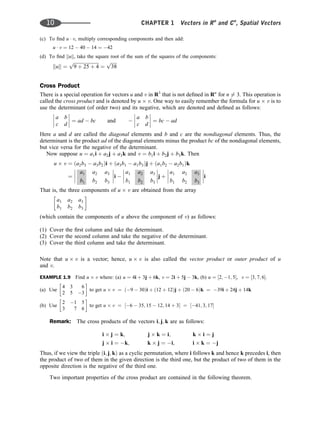
![(a) The formula for the normal vector to a surface Fðx; y; zÞ ¼ 0 is
Nðx; y; zÞ ¼ Fxi þ Fyj þ Fzk
where Fx, Fy, Fz are the partial derivatives. Using Fðx; y; zÞ ¼ xy2
þ 2yz 16, we obtain
Fx ¼ y2
; Fy ¼ 2xy þ 2z; Fz ¼ 2y
Thus, Nðx; y; zÞ ¼ y2
i þ ð2xy þ 2zÞj þ 2yk.
(b) The normal to the surface S at the point P is
NðPÞ ¼ Nð1; 2; 3Þ ¼ 4i þ 10j þ 4k
Hence, N ¼ 2i þ 5j þ 2k is also normal to S at P. Thus an equation of H has the form 2x þ 5y þ 2z ¼ c.
Substitute P in this equation to obtain c ¼ 18. Thus the tangent plane H to S at P is 2x þ 5y þ 2z ¼ 18.
1.24. Evaluate the following determinants and negative of determinants of order two:
(a) (i)
3 4
5 9
, (ii)
2 1
4 3
, (iii)
4 5
3 2
(b) (i)
3 6
4 2
, (ii)
7 5
3 2
, (iii)
4 1
8 3
Use
a b
c d
¼ ad bc and
a b
c d
¼ bc ad. Thus,
(a) (i) 27 20 ¼ 7, (ii) 6 þ 4 ¼ 10, (iii) 8 þ 15 ¼ 7:
(b) (i) 24 6 ¼ 18, (ii) 15 14 ¼ 29, (iii) 8 þ 12 ¼ 4:
1.25. Let u ¼ 2i 3j þ 4k, v ¼ 3i þ j 2k, w ¼ i þ 5j þ 3k.
Find: (a) u v, (b) u w
(a) Use
2 3 4
3 1 2
to get u v ¼ ð6 4Þi þ ð12 þ 4Þj þ ð2 þ 9Þk ¼ 2i þ 16j þ 11k:
(b) Use
2 3 4
1 5 3
to get u w ¼ ð9 20Þi þ ð4 6Þj þ ð10 þ 3Þk ¼ 29i 2j þ 13k:
1.26. Find u v, where: (a) u ¼ ð1; 2; 3Þ, v ¼ ð4; 5; 6Þ; (b) u ¼ ð4; 7; 3Þ, v ¼ ð6; 5; 2Þ.
(a) Use
1 2 3
4 5 6
to get u v ¼ ½12 15; 12 6; 5 8 ¼ ½3; 6; 3:
(b) Use
4 7 3
6 5 2
to get u v ¼ ½14 þ 15; 18 þ 8; 20 42 ¼ ½29; 26; 22:
1.27. Find a unit vector u orthogonal to v ¼ ½1; 3; 4 and w ¼ ½2; 6; 5.
First find v w, which is orthogonal to v and w.
The array
1 3 4
2 6 5
gives v w ¼ ½15 þ 24; 8 þ 5; 6 61 ¼ ½9; 13; 12:
Normalize v w to get u ¼ ½9=
ffiffiffiffiffiffiffiffi
394
p
, 13=
ffiffiffiffiffiffiffiffi
394
p
, 12=
ffiffiffiffiffiffiffiffi
394
p
:
1.28. Let u ¼ ða1; a2; a3Þ and v ¼ ðb1; b2; b3Þ so u v ¼ ða2b3 a3b2; a3b1 a1b3; a1b2 a2b1Þ.
Prove:
(a) u v is orthogonal to u and v [Theorem 1.5(a)].
(b) ku vk2
¼ ðu uÞðv vÞ ðu vÞ2
(Lagrange’s identity).
CHAPTER 1 Vectors in Rn
and Cn
, Spatial Vectors 19](https://image.slidesharecdn.com/linearalgebra4thedition-231030053714-df1faee2/85/Linear_Algebra-_4th_Edition-pdf-26-320.jpg)
![1.48. Write v ¼ ð2; 5Þ as a linear combination of u1 and u2, where:
(a) u1 ¼ ð1; 2Þ and u2 ¼ ð3; 5Þ;
(b) u1 ¼ ð3; 4Þ and u2 ¼ ð2; 3Þ.
1.49. Write v ¼
9
3
16
2
4
3
5 as a linear combination of u1 ¼
1
3
3
2
4
3
5, u2 ¼
2
5
1
2
4
3
5, u3 ¼
4
2
3
2
4
3
5.
1.50. Find k so that u and v are orthogonal, where:
(a) u ¼ ð3; k; 2Þ, v ¼ ð6; 4; 3Þ;
(b) u ¼ ð5; k; 4; 2Þ, v ¼ ð1; 3; 2; 2kÞ;
(c) u ¼ ð1; 7; k þ 2; 2Þ, v ¼ ð3; k; 3; kÞ.
Located Vectors, Hyperplanes, Lines in Rn
1.51. Find the vector v identified with the directed line segment PQ
!
for the points:
(a) Pð2; 3; 7Þ and Qð1; 6; 5Þ in R3
;
(b) Pð1; 8; 4; 6Þ and Qð3; 5; 2; 4Þ in R4
.
1.52. Find an equation of the hyperplane H in R4
that:
(a) contains Pð1; 2; 3; 2Þ and is normal to u ¼ ½2; 3; 5; 6;
(b) contains Pð3; 1; 2; 5Þ and is parallel to 2x1 3x2 þ 5x3 7x4 ¼ 4.
1.53. Find a parametric representation of the line in R4
that:
(a) passes through the points Pð1; 2; 1; 2Þ and Qð3; 5; 7; 9Þ;
(b) passes through Pð1; 1; 3; 3Þ and is perpendicular to the hyperplane 2x1 þ 4x2 þ 6x3 8x4 ¼ 5.
Spatial Vectors (Vectors in R3
), ijk Notation
1.54. Given u ¼ 3i 4j þ 2k, v ¼ 2i þ 5j 3k, w ¼ 4i þ 7j þ 2k. Find:
(a) 2u 3v; (b) 3u þ 4v 2w; (c) u v, u w, v w; (d) kuk, kvk, kwk.
1.55. Find the equation of the plane H:
(a) with normal N ¼ 3i 4j þ 5k and containing the point Pð1; 2; 3Þ;
(b) parallel to 4x þ 3y 2z ¼ 11 and containing the point Qð2; 1; 3Þ.
1.56. Find the (parametric) equation of the line L:
(a) through the point Pð2; 5; 3Þ and in the direction of v ¼ 4i 5j þ 7k;
(b) perpendicular to the plane 2x 3y þ 7z ¼ 4 and containing Pð1; 5; 7Þ.
1.57. Consider the following curve C in R3
where 0 t 5:
FðtÞ ¼ t3
i t2
j þ ð2t 3Þk
(a) Find the point P on C corresponding to t ¼ 2.
(b) Find the initial point Q and the terminal point Q 0
.
(c) Find the unit tangent vector T to the curve C when t ¼ 2.
1.58. Consider a moving body B whose position at time t is given by RðtÞ ¼ t2
i þ t3
j þ 3tk. [Then
VðtÞ ¼ dRðtÞ=dt and AðtÞ ¼ dVðtÞ=dt denote, respectively, the velocity and acceleration of B.] When
t ¼ 1, find for the body B:
(a) position; (b) velocity v; (c) speed s; (d) acceleration a.
CHAPTER 1 Vectors in Rn
and Cn
, Spatial Vectors 23](https://image.slidesharecdn.com/linearalgebra4thedition-231030053714-df1faee2/85/Linear_Algebra-_4th_Edition-pdf-30-320.jpg)
![1.71. Prove: For any vectors u; v; w in Cn
:
(a) ðu þ vÞ w ¼ u w þ v w, (b) w ðu þ vÞ ¼ w u þ w v.
1.72. Prove that the norm in Cn
satisfies the following laws:
½N1 For any vector u, kuk 0; and kuk ¼ 0 if and only if u ¼ 0.
½N2 For any vector u and complex number z, kzuk ¼ jzjkuk.
½N3 For any vectors u and v, ku þ vk kuk þ kvk.
ANSWERS TO SUPPLEMENTARY PROBLEMS
1.41. (a) ð3; 16; 4Þ; (b) (6,1,35); (c) 3; 12; 8; (d)
ffiffiffiffiffi
21
p
,
ffiffiffiffiffi
35
p
,
ffiffiffiffiffi
14
p
;
(e) 3=
ffiffiffiffiffi
21
p ffiffiffiffiffi
35
p
; ( f )
ffiffiffiffiffi
62
p
; (g) 3
35 ð3; 5; 1Þ ¼ ð 9
35, 15
35, 3
35)
1.42. (Column vectors) (a) ð1; 7; 22Þ; (b) ð1; 26; 29Þ; (c) 15; 27; 34;
(d)
ffiffiffiffiffi
26
p
,
ffiffiffiffiffi
30
p
; (e) 15=ð
ffiffiffiffiffi
26
p ffiffiffiffiffi
30
p
Þ; ( f )
ffiffiffiffiffi
86
p
; (g) 15
30 v ¼ ð1; 1
2 ; 5
2Þ
1.43. (a) ð13; 14; 13; 45; 0Þ; (b) ð20; 29; 22; 16; 23Þ; (c) 6; (d)
ffiffiffiffiffi
90
p
;
ffiffiffiffiffi
95
p
;
(e) 6
95 v; ( f )
ffiffiffiffiffiffiffiffi
167
p
1.44. (a) ð5=
ffiffiffiffiffi
76
p
; 9=
ffiffiffiffiffi
76
p
Þ; (b) ð1
5 ; 2
5 ; 2
5 ; 4
5Þ; (c) ð6=
ffiffiffiffiffiffiffiffi
133
p
; 4
ffiffiffiffiffiffiffiffi
133
p
; 9
ffiffiffiffiffiffiffiffi
133
p
Þ
1.45. (a) 3; 13;
ffiffiffiffiffiffiffiffi
120
p
; 9
1.46. (a) x ¼ 3; y ¼ 5; (b) x ¼ 0; y ¼ 0, and x ¼ 1; y ¼ 2
1.47. x ¼ 3; y ¼ 3; z ¼ 3
2
1.48. (a) v ¼ 5u1 u2; (b) v ¼ 16u1 23u2
1.49. v ¼ 3u1 u2 þ 2u3
1.50. (a) 6; (b) 3; (c) 3
2
1.51. (a) v ¼ ½1; 9; 2; (b) [2; 3; 6; 10]
1.52. (a) 2x1 þ 3x2 5x3 þ 6x4 ¼ 35; (b) 2x1 3x2 þ 5x3 7x4 ¼ 16
1.53. (a) ½2t þ 1; 7t þ 2; 6t þ 1; 11t þ 2; (b) ½2t þ 1; 4t þ 1; 6t þ 3; 8t þ 3
1.54. (a) 23j þ 13k; (b) 9i 6j 10k; (c) 20; 12; 37; (d)
ffiffiffiffiffi
29
p
;
ffiffiffiffiffi
38
p
;
ffiffiffiffiffi
69
p
1.55. (a) 3x 4y þ 5z ¼ 20; (b) 4x þ 3y 2z ¼ 1
1.56. (a) ½4t þ 2; 5t þ 5; 7t 3; (b) ½2t þ 1; 3t 5; 7t þ 7
1.57. (a) P ¼ Fð2Þ ¼ 8i 4j þ k; (b) Q ¼ Fð0Þ ¼ 3k, Q0
¼ Fð5Þ ¼ 125i 25j þ 7k;
(c) T ¼ ð6i 2j þ kÞ=
ffiffiffiffiffi
41
p
1.58. (a) i þ j þ 2k; (b) 2i þ 3j þ 2k; (c)
ffiffiffiffiffi
17
p
; (d) 2i þ 6j
1.59. (a) N ¼ 6i þ 7j þ 9k, 6x þ 7y þ 9z ¼ 45; (b) N ¼ 6i 12j 10k, 3x 6y 5z ¼ 16
CHAPTER 1 Vectors in Rn
and Cn
, Spatial Vectors 25](https://image.slidesharecdn.com/linearalgebra4thedition-231030053714-df1faee2/85/Linear_Algebra-_4th_Edition-pdf-32-320.jpg)
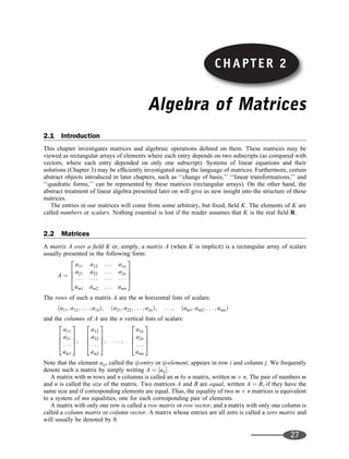

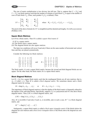
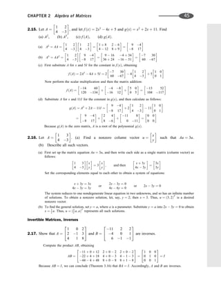
![DEFINITION: Suppose A ¼ ½aik and B ¼ ½bkj are matrices such that the number of columns of A is
equal to the number of rows of B; say, A is an m p matrix and B is a p n matrix.
Then the product AB is the m n matrix whose ij-entry is obtained by multiplying the
ith row of A by the jth column of B. That is,
a11 . . . a1p
: . . . :
ai1 . . . aip
: . . . :
am1 . . . amp
2
6
6
6
6
4
3
7
7
7
7
5
b11 . . . b1j . . . b1n
: . . . : . . . :
: . . . : . . . :
: . . . : . . . :
bp1 . . . bpj . . . bpn
2
6
6
6
6
4
3
7
7
7
7
5
¼
c11 . . . c1n
: . . . :
: cij :
: . . . :
cm1 . . . cmn
2
6
6
6
6
4
3
7
7
7
7
5
where cij ¼ ai1b1j þ ai2b2j þ þ aipbpj ¼
P
p
k¼1
aikbkj
The product AB is not defined if A is an m p matrix and B is a q n matrix, where p 6¼ q.
EXAMPLE 2.5
(a) Find AB where A ¼
1 3
2 1
and B ¼
2 0 4
5 2 6
.
Because A is 2 2 and B is 2 3, the product AB is defined and AB is a 2 3 matrix. To obtain
the first row of the product matrix AB, multiply the first row [1, 3] of A by each column of B,
2
5
;
0
2
;
4
6
respectively. That is,
AB ¼
2 þ 15 0 6 4 þ 18
¼
17 6 14
To obtain the second row of AB, multiply the second row ½2; 1 of A by each column of B. Thus,
AB ¼
17 6 14
4 5 0 þ 2 8 6
¼
17 6 14
1 2 14
(b) Suppose A ¼
1 2
3 4
and B ¼
5 6
0 2
. Then
AB ¼
5 þ 0 6 4
15 þ 0 18 8
¼
5 2
15 10
and BA ¼
5 þ 18 10 þ 24
0 6 0 8
¼
23 34
6 8
The above example shows that matrix multiplication is not commutative—that is, in general,
AB 6¼ BA. However, matrix multiplication does satisfy the following properties.
THEOREM 2.2: Let A; B; C be matrices. Then, whenever the products and sums are defined,
(i) ðABÞC ¼ AðBCÞ (associative law),
(ii) AðB þ CÞ ¼ AB þ AC (left distributive law),
(iii) ðB þ CÞA ¼ BA þ CA (right distributive law),
(iv) kðABÞ ¼ ðkAÞB ¼ AðkBÞ, where k is a scalar.
We note that 0A ¼ 0 and B0 ¼ 0, where 0 is the zero matrix.
CHAPTER 2 Algebra of Matrices 31](https://image.slidesharecdn.com/linearalgebra4thedition-231030053714-df1faee2/85/Linear_Algebra-_4th_Edition-pdf-38-320.jpg)
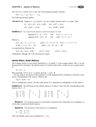
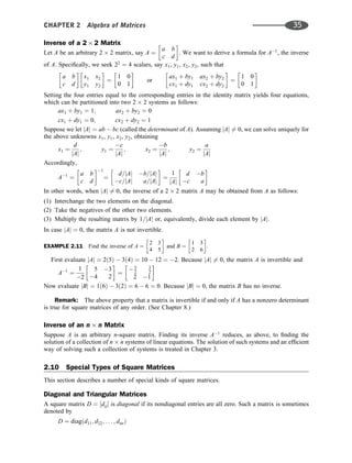
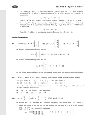
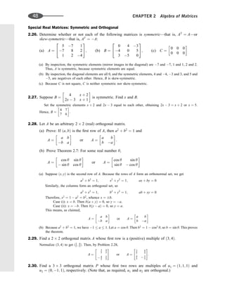
![2.8 Powers of Matrices, Polynomials in Matrices
Let A be an n-square matrix over a field K. Powers of A are defined as follows:
A2
¼ AA; A3
¼ A2
A; . . . ; Anþ1
¼ An
A; . . . ; and A0
¼ I
Polynomials in the matrix A are also defined. Specifically, for any polynomial
f ðxÞ ¼ a0 þ a1x þ a2x2
þ þ anxn
where the ai are scalars in K, f ðAÞ is defined to be the following matrix:
f ðAÞ ¼ a0I þ a1A þ a2A2
þ þ anAn
[Note that f ðAÞ is obtained from f ðxÞ by substituting the matrix A for the variable x and substituting the
scalar matrix a0I for the scalar a0.] If f ðAÞ is the zero matrix, then A is called a zero or root of f ðxÞ.
EXAMPLE 2.9 Suppose A ¼
1 2
3 4
. Then
A2
¼
1 2
3 4
1 2
3 4
¼
7 6
9 22
and A3
¼ A2
A ¼
7 6
9 22
1 2
3 4
¼
11 38
57 106
Suppose f ðxÞ ¼ 2x2
3x þ 5 and gðxÞ ¼ x2
þ 3x 10. Then
f ðAÞ ¼ 2
7 6
9 22
3
1 2
3 4
þ 5
1 0
0 1
¼
16 18
27 61
gðAÞ ¼
7 6
9 22
þ 3
1 2
3 4
10
1 0
0 1
¼
0 0
0 0
Thus, A is a zero of the polynomial gðxÞ.
2.9 Invertible (Nonsingular) Matrices
A square matrix A is said to be invertible or nonsingular if there exists a matrix B such that
AB ¼ BA ¼ I
where I is the identity matrix. Such a matrix B is unique. That is, if AB1 ¼ B1A ¼ I and AB2 ¼ B2A ¼ I,
then
B1 ¼ B1I ¼ B1ðAB2Þ ¼ ðB1AÞB2 ¼ IB2 ¼ B2
We call such a matrix B the inverse of A and denote it by A1
. Observe that the above relation is
symmetric; that is, if B is the inverse of A, then A is the inverse of B.
EXAMPLE 2.10 Suppose that A ¼
2 5
1 3
and B ¼
3 5
1 2
. Then
AB ¼
6 5 10 þ 10
3 3 5 þ 6
¼
1 0
0 1
and BA ¼
6 5 15 15
2 þ 2 5 þ 6
¼
1 0
0 1
Thus, A and B are inverses.
It is known (Theorem 3.16) that AB ¼ I if and only if BA ¼ I. Thus, it is necessary to test only one
product to determine whether or not two given matrices are inverses. (See Problem 2.17.)
Now suppose A and B are invertible. Then AB is invertible and ðABÞ1
¼ B1
A1
. More generally, if
A1; A2; . . . ; Ak are invertible, then their product is invertible and
ðA1A2 . . . AkÞ1
¼ A1
k . . . A1
2 A1
1
the product of the inverses in the reverse order.
34 CHAPTER 2 Algebra of Matrices](https://image.slidesharecdn.com/linearalgebra4thedition-231030053714-df1faee2/85/Linear_Algebra-_4th_Edition-pdf-41-320.jpg)
![where some or all the dii may be zero. For example,
3 0 0
0 7 0
0 0 2
2
4
3
5;
4 0
0 5
;
6
0
9
8
2
6
6
4
3
7
7
5
are diagonal matrices, which may be represented, respectively, by
diagð3; 7; 2Þ; diagð4; 5Þ; diagð6; 0; 9; 8Þ
(Observe that patterns of 0’s in the third matrix have been omitted.)
A square matrix A ¼ ½aij is upper triangular or simply triangular if all entries below the (main)
diagonal are equal to 0—that is, if aij ¼ 0 for i j. Generic upper triangular matrices of orders 2, 3, 4 are
as follows:
a11 a12
0 a22
;
b11 b12 b13
b22 b23
b33
2
4
3
5;
c11 c12 c13 c14
c22 c23 c24
c33 c34
c44
2
6
6
4
3
7
7
5
(As with diagonal matrices, it is common practice to omit patterns of 0’s.)
The following theorem applies.
THEOREM 2.5: Suppose A ¼ ½aij and B ¼ ½bij are n n (upper) triangular matrices. Then
(i) A þ B, kA, AB are triangular with respective diagonals:
ða11 þ b11; . . . ; ann þ bnnÞ; ðka11; . . . ; kannÞ; ða11b11; . . . ; annbnnÞ
(ii) For any polynomial f ðxÞ, the matrix f ðAÞ is triangular with diagonal
ð f ða11Þ; f ða22Þ; . . . ; f ðannÞÞ
(iii) A is invertible if and only if each diagonal element aii 6¼ 0, and when A1
exists
it is also triangular.
A lower triangular matrix is a square matrix whose entries above the diagonal are all zero. We note
that Theorem 2.5 is true if we replace ‘‘triangular’’ by either ‘‘lower triangular’’ or ‘‘diagonal.’’
Remark: A nonempty collection A of matrices is called an algebra (of matrices) if A is closed
under the operations of matrix addition, scalar multiplication, and matrix multiplication. Clearly, the
square matrices with a given order form an algebra of matrices, but so do the scalar, diagonal, triangular,
and lower triangular matrices.
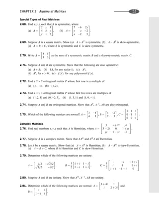
Special Real Square Matrices: Symmetric, Orthogonal, Normal
[Optional until Chapter 12]
Suppose now A is a square matrix with real entries—that is, a real square matrix. The relationship
between A and its transpose AT
yields important kinds of matrices.
(a) Symmetric Matrices
A matrix A is symmetric if AT
¼ A. Equivalently, A ¼ ½aij is symmetric if symmetric elements (mirror
elements with respect to the diagonal) are equal—that is, if each aij ¼ aji.
A matrix A is skew-symmetric if AT
¼ A or, equivalently, if each aij ¼ aji. Clearly, the diagonal
elements of such a matrix must be zero, because aii ¼ aii implies aii ¼ 0.
(Note that a matrix A must be square if AT
¼ A or AT
¼ A.)
36 CHAPTER 2 Algebra of Matrices](https://image.slidesharecdn.com/linearalgebra4thedition-231030053714-df1faee2/85/Linear_Algebra-_4th_Edition-pdf-43-320.jpg)
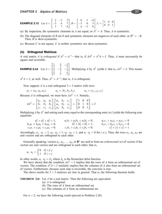
![THEOREM 2.7: Let A be a real 2 2 orthogonal matrix. Then, for some real number y,
A ¼
cos y sin y
sin y cos y
or A ¼
cos y sin y
sin y cos y
(c) Normal Matrices
A real matrix A is normal if it commutes with its transpose AT
—that is, if AAT
¼ AT
A. If A is symmetric,
orthogonal, or skew-symmetric, then A is normal. There are also other normal matrices.
EXAMPLE 2.14 Let A ¼
6 3
3 6
. Then
AAT
¼
6 3
3 6
6 3
3 6
¼
45 0
0 45
and AT
A ¼
6 3
3 6
6 3
3 6
¼
45 0
0 45
Because AAT
¼ AT
A, the matrix A is normal.
2.11 Complex Matrices
Let A be a complex matrix—that is, a matrix with complex entries. Recall (Section 1.7) that if z ¼ a þ bi
is a complex number, then
z ¼ a bi is its conjugate. The conjugate of a complex matrix A, written
A, is
the matrix obtained from A by taking the conjugate of each entry in A. That is, if A ¼ ½aij, then
A ¼ ½bij,
where bij ¼
aij. (We denote this fact by writing
A ¼ ½
aij.)
The two operations of transpose and conjugation commute for any complex matrix A, and the special
notation AH
is used for the conjugate transpose of A. That is,
AH
¼ ð
AÞT
¼ ðAT Þ
Note that if A is real, then AH
¼ AT
. [Some texts use A* instead of AH
:]
EXAMPLE 2.15 Let A ¼
2 þ 8i 5 3i 4 7i
6i 1 4i 3 þ 2i
. Then AH
¼
2 8i 6i
5 þ 3i 1 þ 4i
4 þ 7i 3 2i
2
4
3
5.
Special Complex Matrices: Hermitian, Unitary, Normal [Optional until Chapter 12]
Consider a complex matrix A. The relationship between A and its conjugate transpose AH
yields
important kinds of complex matrices (which are analogous to the kinds of real matrices described above).
A complex matrix A is said to be Hermitian or skew-Hermitian according as to whether
AH
¼ A or AH
¼ A:
Clearly, A ¼ ½aij is Hermitian if and only if symmetric elements are conjugate—that is, if each
aij ¼
aji—in which case each diagonal element aii must be real. Similarly, if A is skew-symmetric,
then each diagonal element aii ¼ 0. (Note that A must be square if AH
¼ A or AH
¼ A.)
A complex matrix A is unitary if AH
A1
¼ A1
AH
¼ I—that is, if
AH
¼ A1
:
Thus, A must necessarily be square and invertible. We note that a complex matrix A is unitary if and only
if its rows (columns) form an orthonormal set relative to the dot product of complex vectors.
A complex matrix A is said to be normal if it commutes with AH
—that is, if
AAH
¼ AH
A
38 CHAPTER 2 Algebra of Matrices](https://image.slidesharecdn.com/linearalgebra4thedition-231030053714-df1faee2/85/Linear_Algebra-_4th_Edition-pdf-45-320.jpg)
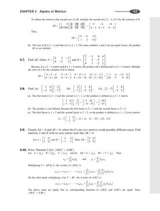
![EXAMPLE 2.17 Determine which of the following square block matrices are upper diagonal, lower
diagonal, or diagonal:
A ¼
1 2 0
3 4 5
0 0 6
2
4
3
5; B ¼
1 0 0 0
2 3 4 0
5 0 6 0
0 7 8 9
2
6
6
4
3
7
7
5; C ¼
1 0 0
0 2 3
0 4 5
2
4
3
5; D ¼
1 2 0
3 4 5
0 6 7
2
4
3
5
(a) A is upper triangular because the block below the diagonal is a zero block.
(b) B is lower triangular because all blocks above the diagonal are zero blocks.
(c) C is diagonal because the blocks above and below the diagonal are zero blocks.
(d) D is neither upper triangular nor lower triangular. Also, no other partitioning of D will make it into
either a block upper triangular matrix or a block lower triangular matrix.
SOLVED PROBLEMS
Matrix Addition and Scalar Multiplication
2.1 Given A ¼
1 2 3
4 5 6
and B ¼
3 0 2
7 1 8
, find:
(a) A þ B, (b) 2A 3B.
(a) Add the corresponding elements:
A þ B ¼
1 þ 3 2 þ 0 3 þ 2
4 7 5 þ 1 6 þ 8
¼
4 2 5
3 6 2
(b) First perform the scalar multiplication and then a matrix addition:
2A 3B ¼
2 4 6
8 10 12
þ
9 0 6
21 3 24
¼
7 4 0
29 7 36
(Note that we multiply B by 3 and then add, rather than multiplying B by 3 and subtracting. This usually
prevents errors.)
2.2. Find x; y; z; t where 3
x y
z t
¼
x 6
1 2t
þ
4 x þ y
z þ t 3
:
Write each side as a single equation:
3x 3y
3z 3t
¼
x þ 4 x þ y þ 6
z þ t 1 2t þ 3
Set corresponding entries equal to each other to obtain the following system of four equations:
3x ¼ x þ 4; 3y ¼ x þ y þ 6; 3z ¼ z þ t 1; 3t ¼ 2t þ 3
or 2x ¼ 4; 2y ¼ 6 þ x; 2z ¼ t 1; t ¼ 3
The solution is x ¼ 2, y ¼ 4, z ¼ 1, t ¼ 3.
2.3. Prove Theorem 2.1 (i) and (v): (i) ðA þ BÞ þ C ¼ A þ ðB þ CÞ, (v) kðA þ BÞ ¼ kA þ kB.
Suppose A ¼ ½aij, B ¼ ½bij, C ¼ ½cij. The proof reduces to showing that corresponding ij-entries
in each side of each matrix equation are equal. [We prove only (i) and (v), because the other parts
of Theorem 2.1 are proved similarly.]
CHAPTER 2 Algebra of Matrices 41](https://image.slidesharecdn.com/linearalgebra4thedition-231030053714-df1faee2/85/Linear_Algebra-_4th_Edition-pdf-48-320.jpg)
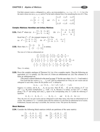
![2.18. Find the inverse, if possible, of each matrix:
(a) A ¼
5 3
4 2
; (b) B ¼
2 3
1 3
; (c)
2 6
3 9
:
Use the formula for the inverse of a 2 2 matrix appearing in Section 2.9.
(a) First find jAj ¼ 5ð2Þ 3ð4Þ ¼ 10 12 ¼ 2. Next interchange the diagonal elements, take the negatives
of the nondiagonal elements, and multiply by 1=jAj:
A1
¼
1
2
2 3
4 5
¼
1 3
2
2 5
2
#
(b) First find jBj ¼ 2ð3Þ ð3Þð1Þ ¼ 6 þ 3 ¼ 9. Next interchange the diagonal elements, take the negatives
of the nondiagonal elements, and multiply by 1=jBj:
B1
¼
1
9
3 3
1 2
¼
1
3
1
3
1
9
2
9
#
(c) First find jCj ¼ 2ð9Þ 6ð3Þ ¼ 18 18 ¼ 0. Because jCj ¼ 0; C has no inverse.
2.19. Let A ¼
1 1 1
0 1 2
1 2 4
2
6
6
4
3
7
7
5. Find A1
¼
x1 x2 x3
y1 y2 y3
z1 z2 z3
2
4
3
5.
Multiplying A by A1
and setting the nine entries equal to the nine entries of the identity matrix I yields the
following three systems of three equations in three of the unknowns:
x1 þ y1 þ z1 ¼ 1 x2 þ y2 þ z2 ¼ 0 x3 þ y3 þ z3 ¼ 0
y1 þ 2z1 ¼ 0 y2 þ 2z2 ¼ 1 y3 þ 2z3 ¼ 0
x1 þ 2y1 þ 4z1 ¼ 0 x2 þ 2y2 þ 4z2 ¼ 0 x3 þ 2y3 þ 4z3 ¼ 1
[Note that A is the coefficient matrix for all three systems.]
Solving the three systems for the nine unknowns yields
x1 ¼ 0; y1 ¼ 2; z1 ¼ 1; x2 ¼ 2; y2 ¼ 3; z2 ¼ 1; x3 ¼ 1; y3 ¼ 2; z3 ¼ 1
Thus; A1
¼
0 2 1
2 3 2
1 1 1
2
6
4
3
7
5
(Remark: Chapter 3 gives an efficient way to solve the three systems.)
2.20. Let A and B be invertible matrices (with the same size). Show that AB is also invertible and
ðABÞ1
¼ B1
A1
. [Thus, by induction, ðA1A2 . . . AmÞ1
¼ A1
m . . . A1
2 A1
1 .]
Using the associativity of matrix multiplication, we get
ðABÞðB1
A1
Þ ¼ AðBB1
ÞA1
¼ AIA1
¼ AA1
¼ I
ðB1
A1
ÞðABÞ ¼ B1
ðA1
AÞB ¼ A1
IB ¼ B1
B ¼ I
Thus, ðABÞ1
¼ B1
A1
.
46 CHAPTER 2 Algebra of Matrices](https://image.slidesharecdn.com/linearalgebra4thedition-231030053714-df1faee2/85/Linear_Algebra-_4th_Edition-pdf-53-320.jpg)
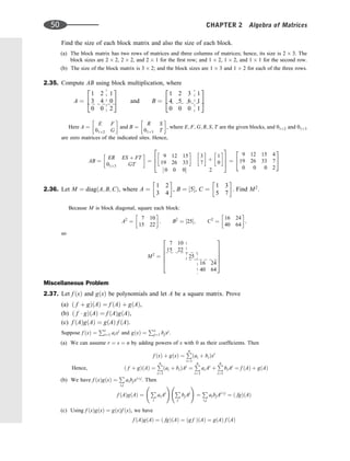
![Diagonal and Triangular Matrices
2.21. Write out the diagonal matrices A ¼ diagð4; 3; 7Þ, B ¼ diagð2; 6Þ, C ¼ diagð3; 8; 0; 5Þ.
Put the given scalars on the diagonal and 0’s elsewhere:
A ¼
4 0 0
0 3 0
0 0 7
2
4
3
5; B ¼
2 0
0 6
; C ¼
3
8
0
5
2
6
6
4
3
7
7
5
2.22. Let A ¼ diagð2; 3; 5Þ and B ¼ diagð7; 0; 4Þ. Find
(a) AB, A2
, B2
; (b) f ðAÞ, where f ðxÞ ¼ x2
þ 3x 2; (c) A1
and B1
.
(a) The product matrix AB is a diagonal matrix obtained by multiplying corresponding diagonal entries; hence,
AB ¼ diagð2ð7Þ; 3ð0Þ; 5ð4ÞÞ ¼ diagð14; 0; 20Þ
Thus, the squares A2
and B2
are obtained by squaring each diagonal entry; hence,
A2
¼ diagð22
; 32
; 52
Þ ¼ diagð4; 9; 25Þ and B2
¼ diagð49; 0; 16Þ
(b) f ðAÞ is a diagonal matrix obtained by evaluating f ðxÞ at each diagonal entry. We have
f ð2Þ ¼ 4 þ 6 2 ¼ 8; f ð3Þ ¼ 9 þ 9 2 ¼ 16; f ð5Þ ¼ 25 þ 15 2 ¼ 38
Thus, f ðAÞ ¼ diagð8; 16; 38Þ.
(c) The inverse of a diagonal matrix is a diagonal matrix obtained by taking the inverse (reciprocal)
of each diagonal entry. Thus, A1
¼ diagð1
2 ; 1
3 ; 1
5Þ, but B has no inverse because there is a 0 on the
diagonal.
2.23. Find a 2 2 matrix A such that A2
is diagonal but not A.
Let A ¼
1 2
3 1
. Then A2
¼
7 0
0 7
, which is diagonal.
2.24. Find an upper triangular matrix A such that A3
¼
8 57
0 27
.
Set A ¼
x y
0 z
. Then x3
¼ 8, so x ¼ 2; and z3
¼ 27, so z ¼ 3. Next calculate A3
using x ¼ 2 and y ¼ 3:
A2
¼
2 y
0 3
2 y
0 3
¼
4 5y
0 9
and A3
¼
2 y
0 3
4 5y
0 9
¼
8 19y
0 27
Thus, 19y ¼ 57, or y ¼ 3. Accordingly, A ¼
2 3
0 3
.
2.25. Let A ¼ ½aij and B ¼ ½bij be upper triangular matrices. Prove that AB is upper triangular with
diagonal a11b11, a22b22; . . . ; annbnn.
Let AB ¼ ½cij. Then cij ¼
Pn
k¼1 aikbkj and cii ¼
Pn
k¼1 aikbki. Suppose i j. Then, for any k, either i k or
k j, so that either aik ¼ 0 or bkj ¼ 0. Thus, cij ¼ 0, and AB is upper triangular. Suppose i ¼ j. Then, for
k i, we have aik ¼ 0; and, for k i, we have bki ¼ 0. Hence, cii ¼ aiibii, as claimed. [This proves one part of
Theorem 2.5(i); the statements for A þ B and kA are left as exercises.]
CHAPTER 2 Algebra of Matrices 47](https://image.slidesharecdn.com/linearalgebra4thedition-231030053714-df1faee2/85/Linear_Algebra-_4th_Edition-pdf-54-320.jpg)
![SUPPLEMENTARY PROBLEMS
Algebra of Matrices
Problems 2.38–2.41 refer to the following matrices:
A ¼
1 2
3 4
; B ¼
5 0
6 7
; C ¼
1 3 4
2 6 5
; D ¼
3 7 1
4 8 9
2.38. Find (a) 5A 2B, (b) 2A þ 3B, (c) 2C 3D.
2.39. Find (a) AB and ðABÞC, (b) BC and AðBCÞ. [Note that ðABÞC ¼ AðBCÞ.]
2.40. Find (a) A2
and A3
, (b) AD and BD, (c) CD.
2.41. Find (a) AT
, (b) BT
, (c) ðABÞT
, (d) AT
BT
. [Note that AT
BT
6¼ ðABÞT
.]
Problems 2.42 and 2.43 refer to the following matrices:
A ¼
1 1 2
0 3 4
; B ¼
4 0 3
1 2 3
; C ¼
2 3 0 1
5 1 4 2
1 0 0 3
2
4
3
5; D ¼
2
1
3
2
4
3
5:
2.42. Find (a) 3A 4B, (b) AC, (c) BC, (d) AD, (e) BD, ( f ) CD.
2.43. Find (a) AT
, (b) AT
B, (c) AT
C.
2.44. Let A ¼
1 2
3 6
. Find a 2 3 matrix B with distinct nonzero entries such that AB ¼ 0.
2.45 Let e1 ¼ ½1; 0; 0, e2 ¼ ½0; 1; 0, e3 ¼ ½0; 0; 1, and A ¼
a1 a2 a3 a4
b1 b2 b3 b4
c1 c2 c3 c4
2
4
3
5. Find e1A, e2A, e3A.
2.46. Let ei ¼ ½0; . . . ; 0; 1; 0; . . . ; 0, where 1 is the ith entry. Show
(a) eiA ¼ Ai, ith row of A. (c) If eiA ¼ eiB, for each i, then A ¼ B.
(b) BeT
j ¼ Bj
, jth column of B. (d) If AeT
j ¼ BeT
j , for each j, then A ¼ B.
2.47. Prove Theorem 2.2(iii) and (iv): (iii) ðB þ CÞA ¼ BA þ CA, (iv) kðABÞ ¼ ðkAÞB ¼ AðkBÞ.
2.48. Prove Theorem 2.3: (i) ðA þ BÞT
¼ AT
þ BT
, (ii) ðAT
ÞT
¼ A, (iii) ðkAÞT
¼ kAT
.
2.49. Show (a) If A has a zero row, then AB has a zero row. (b) If B has a zero column, then AB has a
zero column.
Square Matrices, Inverses
2.50. Find the diagonal and trace of each of the following matrices:
(a) A ¼
2 5 8
3 6 7
4 0 1
2
4
3
5, (b) B ¼
1 3 4
6 1 7
2 5 1
2
4
3
5, (c) C ¼
4 3 6
2 5 0
Problems 2.51–2.53 refer to A ¼
2 5
3 1
, B ¼
4 2
1 6
, C ¼
6 4
3 2
.
2.51. Find (a) A2
and A3
, (b) f ðAÞ and gðAÞ, where
f ðxÞ ¼ x3
2x2
5; gðxÞ ¼ x2
3x þ 17:
CHAPTER 2 Algebra of Matrices 51](https://image.slidesharecdn.com/linearalgebra4thedition-231030053714-df1faee2/85/Linear_Algebra-_4th_Edition-pdf-58-320.jpg)
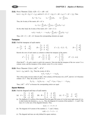
![2.52. Find (a) B2
and B3
, (b) f ðBÞ and gðBÞ, where
f ðxÞ ¼ x2
þ 2x 22; gðxÞ ¼ x2
3x 6:
2.53. Find a nonzero column vector u such that Cu ¼ 4u.
2.54. Find the inverse of each of the following matrices (if it exists):
A ¼
7 4
5 3
; B ¼
2 3
4 5
; C ¼
4 6
2 3
; D ¼
5 2
6 3
2.55. Find the inverses of A ¼
1 1 2
1 2 5
1 3 7
2
4
3
5 and B ¼
1 1 1
0 1 1
1 3 2
2
4
3
5. [Hint: See Problem 2.19.]
2.56. Suppose A is invertible. Show that if AB ¼ AC, then B ¼ C. Give an example of a nonzero matrix
A such that AB ¼ AC but B 6¼ C.
2.57. Find 2 2 invertible matrices A and B such that A þ B 6¼ 0 and A þ B is not invertible.
2.58. Show (a) A is invertible if and only if AT
is invertible. (b) The operations of inversion and
transpose commute; that is, ðAT
Þ1
¼ ðA1
ÞT
. (c) If A has a zero row or zero column, then A is
not invertible.
Diagonal and triangular matrices
2.59. Let A ¼ diagð1; 2; 3Þ and B ¼ diagð2; 5; 0Þ. Find
(a) AB, A2
, B2
; (b) f ðAÞ, where f ðxÞ ¼ x2
þ 4x 3; (c) A1
and B1
.
2.60. Let A ¼
1 2
0 1
and B ¼
1 1 0
0 1 1
0 0 1
2
4
3
5. (a) Find An
. (b) Find Bn
.
2.61. Find all real triangular matrices A such that A2
¼ B, where (a) B ¼
4 21
0 25
, (b) B ¼
1 4
0 9
.
2.62. Let A ¼
5 2
0 k
. Find all numbers k for which A is a root of the polynomial:
(a) f ðxÞ ¼ x2
7x þ 10, (b) gðxÞ ¼ x2
25, (c) hðxÞ ¼ x2
4.
2.63. Let B ¼
1 0
26 27
: Find a matrix A such that A3
¼ B.
2.64. Let B ¼
1 8 5
0 9 5
0 0 4
2
4
3
5. Find a triangular matrix A with positive diagonal entries such that A2
¼ B.
2.65. Using only the elements 0 and 1, find the number of 3 3 matrices that are (a) diagonal,
(b) upper triangular, (c) nonsingular and upper triangular. Generalize to n n matrices.
2.66. Let Dk ¼ kI, the scalar matrix belonging to the scalar k. Show
(a) DkA ¼ kA, (b) BDk ¼ kB, (c) Dk þ Dk0 ¼ Dkþk0 , (d) DkDk0 ¼ Dkk0
2.67. Suppose AB ¼ C, where A and C are upper triangular.
(a) Find 2 2 nonzero matrices A; B; C, where B is not upper triangular.
(b) Suppose A is also invertible. Show that B must also be upper triangular.
52 CHAPTER 2 Algebra of Matrices](https://image.slidesharecdn.com/linearalgebra4thedition-231030053714-df1faee2/85/Linear_Algebra-_4th_Edition-pdf-59-320.jpg)
![2.43. (a) ½1; 0; 1; 3; 2; 4, (b) ½4; 0; 3; 7; 6; 12; 4; 8; 6], (c) not defined
2.44. ½2; 4; 6; 1; 2; 3
2.45. ½a1; a2; a3; a4, ½b1; b2; b3; b4, ½c1; c2; c3; c4
2.50. (a) 2; 6; 1; trðAÞ ¼ 5, (b) 1; 1; 1; trðBÞ ¼ 1, (c) not defined
2.51. (a) ½11; 15; 9; 14, ½67; 40; 24; 59, (b) ½50; 70; 42; 36, gðAÞ ¼ 0
2.52. (a) ½14; 4; 2; 34, ½60; 52; 26; 200, (b) f ðBÞ ¼ 0, ½4; 10; 5; 46
2.53. u ¼ ½2a; aT
2.54. ½3; 4; 5; 7, ½ 5
2 ; 3
2; 2; 1, not defined, ½1; 2
3; 2; 5
3
2.55. ½1; 1; 1; 2; 5; 3; 1; 2; 1, ½1; 1; 0; 1; 3; 1; 1; 4; 1
2.56. A ¼ ½1; 2; 1; 2, B ¼ ½0; 0; 1; 1, C ¼ ½2; 2; 0; 0
2.57. A ¼ ½1; 2; 0; 3; B ¼ ½4; 3; 3; 0
2.58. (c) Hint: Use Problem 2.48
2.59. (a) AB ¼ diagð2; 10; 0Þ, A2
¼ diagð1; 4; 9Þ, B2
¼ diagð4; 25; 0Þ;
(b) f ðAÞ ¼ diagð2; 9; 6Þ; (c) A1
¼ diagð1; 1
2 ; 1
3Þ, C1
does not exist
2.60. (a) ½1; 2n; 0; 1, (b) ½1; n; 1
2 nðn 1Þ; 0; 1; n; 0; 0; 1
2.61. (a) ½2; 3; 0; 5, ½2; 3; 0; 5, ½2; 7; 0; 5, ½2; 7; 0; 5, (b) none
2.62. (a) k ¼ 2, (b) k ¼ 5, (c) none
2.63. ½1; 0; 2; 3
2.64. ½1; 2; 1; 0; 3; 1; 0; 0; 2
2.65. All entries below the diagonal must be 0 to be upper triangular, and all diagonal entries must be 1
to be nonsingular.
(a) 8 ð2n
Þ, (b) 26
ð2nðnþ1Þ=2
Þ, (c) 23
ð2nðn1Þ=2
Þ
2.67. (a) A ¼ ½1; 1; 0; 0, B ¼ ½1; 2; 3; 4, C ¼ ½4; 6; 0; 0
2.68. (a) x ¼ 4, y ¼ 1, z ¼ 3; (b) x ¼ 0, y ¼ 6, z any real number
2.69. (c) Hint: Let B ¼ 1
2 ðA þ AT
Þ and C ¼ 1
2 ðA AT
Þ:
2.70. B ¼ ½4; 3; 3; 3, C ¼ ½0; 2; 2; 0
2.72. (a) ½3
5, 4
5; 4
5, 3
5], (b) ½1=
ffiffiffi
5
p
, 2=
ffiffiffi
5
p
; 2=
ffiffiffi
5
p
, 1=
ffiffiffi
5
p
2.73. (a) ½1=
ffiffiffiffiffi
14
p
, 2=
ffiffiffiffiffi
14
p
, 3=
ffiffiffiffiffi
14
p
; 0; 2=
ffiffiffiffiffi
13
p
, 3=
ffiffiffiffiffi
13
p
; 12=
ffiffiffiffiffiffiffiffi
157
p
, 3=
ffiffiffiffiffiffiffiffi
157
p
, 2=
ffiffiffiffiffiffiffiffi
157
p
(b) ½1=
ffiffiffiffiffi
11
p
, 3=
ffiffiffiffiffi
11
p
, 1=
ffiffiffiffiffi
11
p
; 1=
ffiffiffi
2
p
, 0; 1=
ffiffiffi
2
p
; 3=
ffiffiffiffiffi
22
p
, 2=
ffiffiffiffiffi
22
p
, 3=
ffiffiffiffiffi
22
p
2.75. A; C
CHAPTER 2 Algebra of Matrices 55](https://image.slidesharecdn.com/linearalgebra4thedition-231030053714-df1faee2/85/Linear_Algebra-_4th_Edition-pdf-62-320.jpg)
![2.76. x ¼ 3, y ¼ 0, z ¼ 3
2.78. (c) Hint: Let B ¼ 1
2 ðA þ AH
Þ and C ¼ 1
2 ðA AH
Þ.
2.79. A; B; C
2.81. A
2.82. (a) UV ¼ diagð½7; 6; 17; 10; ½1; 9; 7; 5); (b) no; (c) yes
2.83. A: line between first and second rows (columns);
B: line between second and third rows (columns) and between fourth and fifth rows (columns);
C: C itself—no further partitioning of C is possible.
2.84. (a) M2
¼ diagð½4, ½9; 8; 4; 9, ½9Þ,
M3
¼ diagð½8; ½25; 44; 22; 25, ½27Þ
(b) M2
¼ diagð½3; 4; 8; 11, ½9; 12; 24; 33Þ
M3
¼ diagð½11; 15; 30; 41, ½57; 78; 156; 213Þ
2.85. (a) diagð½7, ½8; 24; 12; 8, ½16Þ, (b) diagð½2; 8; 16; 181], ½8; 20; 40; 48Þ
56 CHAPTER 2 Algebra of Matrices](https://image.slidesharecdn.com/linearalgebra4thedition-231030053714-df1faee2/85/Linear_Algebra-_4th_Edition-pdf-63-320.jpg)

![Then L is a linear combination of L1, L2, L3. As expected, the solution u ¼ ð8; 6; 1; 1Þ of the system is also a
solution of L. That is, substituting u in L, we obtain a true statement:
3ð8Þ þ 5ð6Þ 10ð1Þ þ 29ð1Þ ¼ 25 or 24 þ 30 10 þ 29 ¼ 25 or 9 ¼ 9
The following theorem holds.
THEOREM 3.3: Two systems of linear equations have the same solutions if and only if each equation in
each system is a linear combination of the equations in the other system.
Two systems of linear equations are said to be equivalent if they have the same solutions. The next
subsection shows one way to obtain equivalent systems of linear equations.
Elementary Operations
The following operations on a system of linear equations L1; L2; . . . ; Lm are called elementary operations.
½E1 Interchange two of the equations. We indicate that the equations Li and Lj are interchanged by
writing:
‘‘Interchange Li and Lj’’ or ‘‘Li ! Lj’’
½E2 Replace an equation by a nonzero multiple of itself. We indicate that equation Li is replaced by kLi
(where k 6¼ 0) by writing
‘‘Replace Li by kLi’’ or ‘‘kLi ! Li’’
½E3 Replace an equation by the sum of a multiple of another equation and itself. We indicate that
equation Lj is replaced by the sum of kLi and Lj by writing
‘‘Replace Lj by kLi þ Lj’’ or ‘‘kLi þ Lj ! Lj’’
The arrow ! in ½E2 and ½E3 may be read as ‘‘replaces.’’
The main property of the above elementary operations is contained in the following theorem (proved
in Problem 3.45).
THEOREM 3.4: Suppose a system of m of linear equations is obtained from a system l of linear
equations by a finite sequence of elementary operations. Then m and l have the same
solutions.
Remark: Sometimes (say to avoid fractions when all the given scalars are integers) we may apply
½E2 and ½E3 in one step; that is, we may apply the following operation:
½E Replace equation Lj by the sum of kLi and k0
Lj (where k0
6¼ 0), written
‘‘Replace Lj by kLi þ k0
Lj’’ or ‘‘kLi þ k0
Lj ! Lj’’
We emphasize that in operations ½E3 and [E], only equation Lj is changed.
Gaussian elimination, our main method for finding the solution of a given system of linear
equations, consists of using the above operations to transform a given system into an equivalent
system whose solution can be easily obtained.
The details of Gaussian elimination are discussed in subsequent sections.
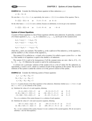
3.4 Small Square Systems of Linear Equations
This section considers the special case of one equation in one unknown, and two equations in two
unknowns. These simple systems are treated separately because their solution sets can be described
geometrically, and their properties motivate the general case.
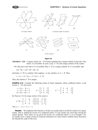
CHAPTER 3 Systems of Linear Equations 61](https://image.slidesharecdn.com/linearalgebra4thedition-231030053714-df1faee2/85/Linear_Algebra-_4th_Edition-pdf-68-320.jpg)
![Linear Equation in One Unknown
The following simple basic result is proved in Problem 3.5.
THEOREM 3.5: Consider the linear equation ax ¼ b.
(i) If a 6¼ 0, then x ¼ b=a is a unique solution of ax ¼ b.
(ii) If a ¼ 0, but b 6¼ 0, then ax ¼ b has no solution.
(iii) If a ¼ 0 and b ¼ 0, then every scalar k is a solution of ax ¼ b.
EXAMPLE 3.4 Solve (a) 4x 1 ¼ x þ 6, (b) 2x 5 x ¼ x þ 3, (c) 4 þ x 3 ¼ 2x þ 1 x.
(a) Rewrite the equation in standard form obtaining 3x ¼ 7. Then x ¼ 7
3 is the unique solution [Theorem 3.5(i)].
(b) Rewrite the equation in standard form, obtaining 0x ¼ 8. The equation has no solution [Theorem 3.5(ii)].
(c) Rewrite the equation in standard form, obtaining 0x ¼ 0. Then every scalar k is a solution [Theorem 3.5(iii)].
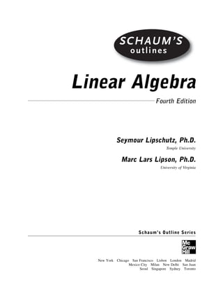
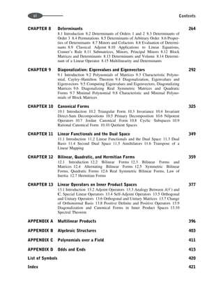
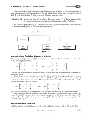
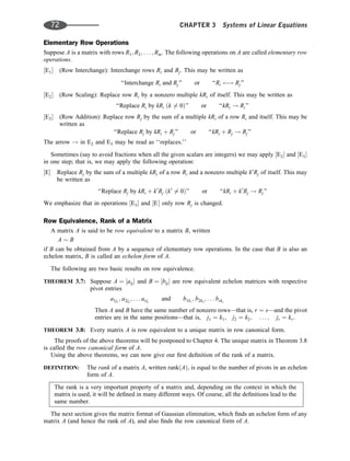
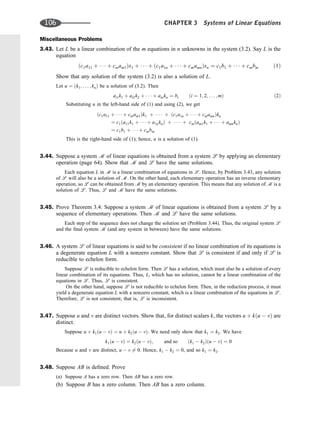
System of Two Linear Equations in Two Unknowns (2 2 System)
Consider a system of two nondegenerate linear equations in two unknowns x and y, which can be put in
the standard form
A1x þ B1y ¼ C1
A2x þ B2y ¼ C2
ð3:4Þ
Because the equations are nondegenerate, A1 and B1 are not both zero, and A2 and B2 are not both zero.
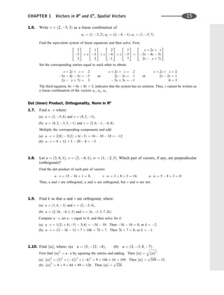
The general solution of the system (3.4) belongs to one of three types as indicated in Fig. 3-1. If R is
the field of scalars, then the graph of each equation is a line in the plane R2
and the three types may be
described geometrically as pictured in Fig. 3-2. Specifically,
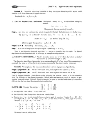
(1) The system has exactly one solution.
Here the two lines intersect in one point [Fig. 3-2(a)]. This occurs when the lines have distinct
slopes or, equivalently, when the coefficients of x and y are not proportional:
A1
A2
6¼
B1
B2
or; equivalently; A1B2 A2B1 6¼ 0
For example, in Fig. 3-2(a), 1=3 6¼ 1=2.
y
L1
x
L2
0
–3 3
–3
3
L x y
L x y
1
2
: – = –
1
: 3 + 2 = 12
6
(a)
y
(b)
L1
x
L2
0 3
–3
3
L x y
L x y
1
2
: + 3 = 3
: 2 + 6 = –
8
6
–3
y
(c)
L L
1 2
and
x
0 3
–3
3
L x y
L x y
1
2
: + 2 = 4
: 2 + 4 = 8
6
–3
Figure 3-2
62 CHAPTER 3 Systems of Linear Equations](https://image.slidesharecdn.com/linearalgebra4thedition-231030053714-df1faee2/85/Linear_Algebra-_4th_Edition-pdf-69-320.jpg)
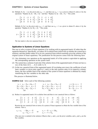
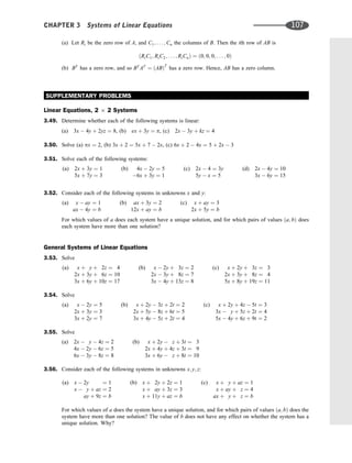
![(2) The system has no solution.
Here the two lines are parallel [Fig. 3-2(b)]. This occurs when the lines have the same slopes but
different y intercepts, or when
A1
A2
¼
B1
B2
6¼
C1
C2
For example, in Fig. 3-2(b), 1=2 ¼ 3=6 6¼ 3=8.
(3) The system has an infinite number of solutions.
Here the two lines coincide [Fig. 3-2(c)]. This occurs when the lines have the same slopes and same
y intercepts, or when the coefficients and constants are proportional,
A1
A2
¼
B1
B2
¼
C1
C2
For example, in Fig. 3-2(c), 1=2 ¼ 2=4 ¼ 4=8.
Remark: The following expression and its value is called a determinant of order two:
A1 B1
A2 B2
¼ A1B2 A2B1
Determinants will be studied in Chapter 8. Thus, the system (3.4) has a unique solution if and only if the
determinant of its coefficients is not zero. (We show later that this statement is true for any square system
of linear equations.)
Elimination Algorithm
The solution to system (3.4) can be obtained by the process of elimination, whereby we reduce the system
to a single equation in only one unknown. Assuming the system has a unique solution, this elimination
algorithm has two parts.
ALGORITHM 3.1: The input consists of two nondegenerate linear equations L1 and L2 in two
unknowns with a unique solution.
Part A. (Forward Elimination) Multiply each equation by a constant so that the resulting coefficients of
one unknown are negatives of each other, and then add the two equations to obtain a new
equation L that has only one unknown.
Part B. (Back-Substitution) Solve for the unknown in the new equation L (which contains only one
unknown), substitute this value of the unknown into one of the original equations, and then
solve to obtain the value of the other unknown.
Part A of Algorithm 3.1 can be applied to any system even if the system does not have a unique
solution. In such a case, the new equation L will be degenerate and Part B will not apply.
EXAMPLE 3.5 (Unique Case). Solve the system
L1: 2x 3y ¼ 8
L2: 3x þ 4y ¼ 5
The unknown x is eliminated from the equations by forming the new equation L ¼ 3L1 þ 2L2. That is, we
multiply L1 by 3 and L2 by 2 and add the resulting equations as follows:
3L1: 6x þ 9y ¼ 24
2L2: 6x þ 8y ¼ 10
Addition : 17y ¼ 34
CHAPTER 3 Systems of Linear Equations 63](https://image.slidesharecdn.com/linearalgebra4thedition-231030053714-df1faee2/85/Linear_Algebra-_4th_Edition-pdf-70-320.jpg)
![We now solve the new equation for y, obtaining y ¼ 2. We substitute y ¼ 2 into one of the original equations, say
L1, and solve for the other unknown x, obtaining
2x 3ð2Þ ¼ 8 or 2x 6 ¼ 8 or 2x ¼ 2 or x ¼ 1
Thus, x ¼ 1, y ¼ 2, or the pair u ¼ ð1; 2Þ is the unique solution of the system. The unique solution is expected,
because 2=3 6¼ 3=4. [Geometrically, the lines corresponding to the equations intersect at the point ð1; 2Þ.]
EXAMPLE 3.6 (Nonunique Cases)
(a) Solve the system
L1: x 3y ¼ 4
L2: 2x þ 6y ¼ 5
We eliminated x from the equations by multiplying L1 by 2 and adding it to L2—that is, by forming the new
equation L ¼ 2L1 þ L2. This yields the degenerate equation
0x þ 0y ¼ 13
which has a nonzero constant b ¼ 13. Thus, this equation and the system have no solution. This is expected,
because 1=ð2Þ ¼ 3=6 6¼ 4=5. (Geometrically, the lines corresponding to the equations are parallel.)
(b) Solve the system
L1: x 3y ¼ 4
L2: 2x þ 6y ¼ 8
We eliminated x from the equations by multiplying L1 by 2 and adding it to L2—that is, by forming the new
equation L ¼ 2L1 þ L2. This yields the degenerate equation
0x þ 0y ¼ 0
where the constant term is also zero. Thus, the system has an infinite number of solutions, which correspond to
the solutions of either equation. This is expected, because 1=ð2Þ ¼ 3=6 ¼ 4=ð8Þ. (Geometrically, the lines
corresponding to the equations coincide.)
To find the general solution, let y ¼ a, and substitute into L1 to obtain
x 3a ¼ 4 or x ¼ 3a þ 4
Thus, the general solution of the system is
x ¼ 3a þ 4; y ¼ a or u ¼ ð3a þ 4; aÞ
where a (called a parameter) is any scalar.
3.5 Systems in Triangular and Echelon Forms
The main method for solving systems of linear equations, Gaussian elimination, is treated in Section 3.6.
Here we consider two simple types of systems of linear equations: systems in triangular form and the
more general systems in echelon form.
Triangular Form
Consider the following system of linear equations, which is in triangular form:
2x1 3x2 þ 5x3 2x4 ¼ 9
5x2 x3 þ 3x4 ¼ 1
7x3 x4 ¼ 3
2x4 ¼ 8
64 CHAPTER 3 Systems of Linear Equations](https://image.slidesharecdn.com/linearalgebra4thedition-231030053714-df1faee2/85/Linear_Algebra-_4th_Edition-pdf-71-320.jpg)
![with the property that
aij ¼ 0 for
ðiÞ i r; j ji
ðiiÞ i r
The entries a1j1
, a2j2
; . . . ; arjr
, which are the leading nonzero elements in their respective rows, are called
the pivots of the echelon matrix.
EXAMPLE 3.9 The following is an echelon matrix whose pivots have been circled:
A ¼
0 2 3 4 5 9 0 7
0 0 0 3 4 1 2 5
0 0 0 0 0 5 7 2
0 0 0 0 0 0 8 6
0 0 0 0 0 0 0 0
2
6
6
6
6
4
3
7
7
7
7
5
Observe that the pivots are in columns C2; C4; C6; C7, and each is to the right of the one above. Using the above
notation, the pivots are
a1j1
¼ 2; a2j2
¼ 3; a3j3
¼ 5; a4j4
¼ 8
where j1 ¼ 2, j2 ¼ 4, j3 ¼ 6, j4 ¼ 7. Here r ¼ 4.
Row Canonical Form
A matrix A is said to be in row canonical form (or row-reduced echelon form) if it is an echelon matrix—
that is, if it satisfies the above properties (1) and (2), and if it satisfies the following additional two
properties:
(3) Each pivot (leading nonzero entry) is equal to 1.
(4) Each pivot is the only nonzero entry in its column.
The major difference between an echelon matrix and a matrix in row canonical form is that in an
echelon matrix there must be zeros below the pivots [Properties (1) and (2)], but in a matrix in row
canonical form, each pivot must also equal 1 [Property (3)] and there must also be zeros above the pivots
[Property (4)].
The zero matrix 0 of any size and the identity matrix I of any size are important special examples of
matrices in row canonical form.
EXAMPLE 3.10
The following are echelon matrices whose pivots have been circled:
2 3 2 0 4 5 6
0 0 0 1 3 2 0
0 0 0 0 0 6 2
0 0 0 0 0 0 0
2
6
6
4
3
7
7
5;
1 2 3
0 0 1
0 0 0
2
4
3
5;
0 1 3 0 0 4
0 0 0 1 0 3
0 0 0 0 1 2
2
4
3
5
The third matrix is also an example of a matrix in row canonical form. The second matrix is not in row canonical
form, because it does not satisfy property (4); that is, there is a nonzero entry above the second pivot in the third
column. The first matrix is not in row canonical form, because it satisfies neither property (3) nor property (4); that
is, some pivots are not equal to 1 and there are nonzero entries above the pivots.
CHAPTER 3 Systems of Linear Equations 71](https://image.slidesharecdn.com/linearalgebra4thedition-231030053714-df1faee2/85/Linear_Algebra-_4th_Edition-pdf-78-320.jpg)
![One can show that row equivalence is an equivalence relation. That is,
(1) A A for any matrix A.
(2) If A B, then B A.
(3) If A B and B C, then A C.
Property (2) comes from the fact that each elementary row operation has an inverse operation of the same
type. Namely,
(i) ‘‘Interchange Ri and Rj’’ is its own inverse.
(ii) ‘‘Replace Ri by kRi’’ and ‘‘Replace Ri by ð1=kÞRi’’ are inverses.
(iii) ‘‘Replace Rj by kRi þ Rj’’ and ‘‘Replace Rj by kRi þ Rj’’ are inverses.
There is a similar result for operation [E] (Problem 3.73).
3.8 Gaussian Elimination, Matrix Formulation
This section gives two matrix algorithms that accomplish the following:
(1) Algorithm 3.3 transforms any matrix A into an echelon form.
(2) Algorithm 3.4 transforms the echelon matrix into its row canonical form.
These algorithms, which use the elementary row operations, are simply restatements of Gaussian
elimination as applied to matrices rather than to linear equations. (The term ‘‘row reduce’’ or simply
‘‘reduce’’ will mean to transform a matrix by the elementary row operations.)
ALGORITHM 3.3 (Forward Elimination): The input is any matrix A. (The algorithm puts 0’s below
each pivot, working from the ‘‘top-down.’’) The output is
an echelon form of A.
Step 1. Find the first column with a nonzero entry. Let j1 denote this column.
(a) Arrange so that a1j1
6¼ 0. That is, if necessary, interchange rows so that a nonzero entry
appears in the first row in column j1.
(b) Use a1j1
as a pivot to obtain 0’s below a1j1
.
Specifically, for i 1:
ð1Þ Set m ¼ aij1
=a1j1
; ð2Þ Replace Ri by mR1 þ Ri
[That is, apply the operation ðaij1
=a1j1
ÞR1 þ Ri ! Ri:]
Step 2. Repeat Step 1 with the submatrix formed by all the rows excluding the first row. Here we let j2
denote the first column in the subsystem with a nonzero entry. Hence, at the end of Step 2, we
have a2j2
6¼ 0.
Steps 3 to r. Continue the above process until a submatrix has only zero rows.
We emphasize that at the end of the algorithm, the pivots will be
a1j1
; a2j2
; . . . ; arjr
where r denotes the number of nonzero rows in the final echelon matrix.
Remark 1: The following number m in Step 1(b) is called the multiplier:
m ¼
aij1
a1j1
¼
entry to be deleted
pivot
CHAPTER 3 Systems of Linear Equations 73](https://image.slidesharecdn.com/linearalgebra4thedition-231030053714-df1faee2/85/Linear_Algebra-_4th_Edition-pdf-80-320.jpg)

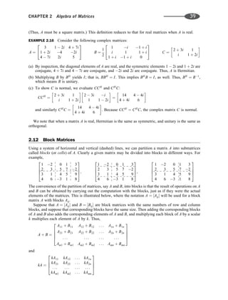
![Matrix Equivalence
A matrix B is equivalent to a matrix A if B can be obtained from A by a sequence of row and column
operations. Alternatively, B is equivalent to A, if there exist nonsingular matrices P and Q such that
B ¼ PAQ. Just like row equivalence, equivalence of matrices is an equivalence relation.
The main result of this subsection (proved in Problem 3.38) is as follows.
THEOREM 3.21: Every m n matrix A is equivalent to a unique block matrix of the form
Ir 0
0 0
where Ir is the r-square identity matrix.
The following definition applies.
DEFINITION: The nonnegative integer r in Theorem 3.18 is called the rank of A, written rankðAÞ.
Note that this definition agrees with the previous definition of the rank of a matrix.
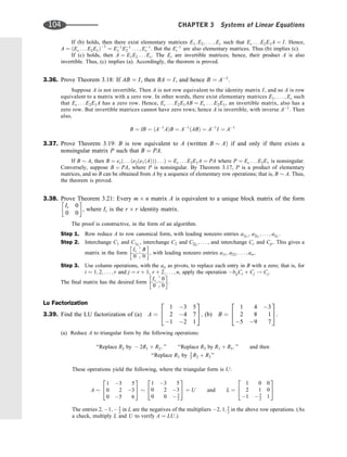
3.13 LU DECOMPOSITION
Suppose A is a nonsingular matrix that can be brought into (upper) triangular form U using only row-
addition operations; that is, suppose A can be triangularized by the following algorithm, which we write
using computer notation.
ALGORITHM 3.6: The input is a matrix A and the output is a triangular matrix U.
Step 1. Repeat for i ¼ 1; 2; . . . ; n 1:
Step 2. Repeat for j ¼ i þ 1, i þ 2; . . . ; n
(a) Set mij : ¼ aij=aii.
(b) Set Rj : ¼ mijRi þ Rj
[End of Step 2 inner loop.]
[End of Step 1 outer loop.]
The numbers mij are called multipliers. Sometimes we keep track of these multipliers by means of the
following lower triangular matrix L:
L ¼
1 0 0 . . . 0 0
m21 1 0 . . . 0 0
m31 m32 1 . . . 0 0
mn1 mn2 mn3 . . . mn;n1 1
2
6
6
6
6
4
3
7
7
7
7
5
That is, L has 1’s on the diagonal, 0’s above the diagonal, and the negative of the multiplier mij as its
ij-entry below the diagonal.
The above matrix L and the triangular matrix U obtained in Algorithm 3.6 give us the classical LU
factorization of such a matrix A. Namely,
THEOREM 3.22: Let A be a nonsingular matrix that can be brought into triangular form U using only
row-addition operations. Then A ¼ LU, where L is the above lower triangular matrix
with 1’s on the diagonal, and U is an upper triangular matrix with no 0’s on the
diagonal.
.........................................................
CHAPTER 3 Systems of Linear Equations 87](https://image.slidesharecdn.com/linearalgebra4thedition-231030053714-df1faee2/85/Linear_Algebra-_4th_Edition-pdf-94-320.jpg)
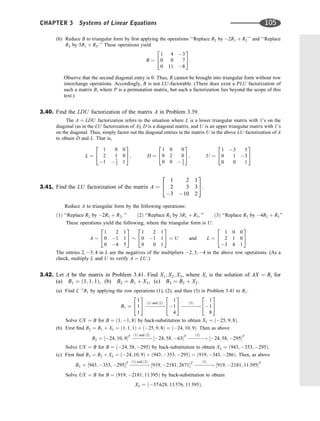
![EXAMPLE 3.22 SupposeA ¼
1 2 3
3 4 13
2 1 5
2
4
3
5.WenotethatA maybereducedtotriangularformbytheoperations
‘‘Replace R2 by 3R1 þ R2’’; ‘‘Replace R3 by 2R1 þ R3’’; and then ‘‘Replace R3 by 3
2 R2 þ R3’’
That is,
A
1 2 3
0 2 4
0 3 1
2
4
3
5
1 2 3
0 2 4
0 0 7
2
4
3
5
This gives us the classical factorization A ¼ LU, where
L ¼
1 0 0
3 1 0
2 3
2 1
2
6
4
3
7
5 and U ¼
1 2 3
0 2 4
0 0 7
2
6
4
3
7
5
We emphasize:
(1) The entries 3; 2; 3
2 in L are the negatives of the multipliers in the above elementary row operations.
(2) U is the triangular form of A.
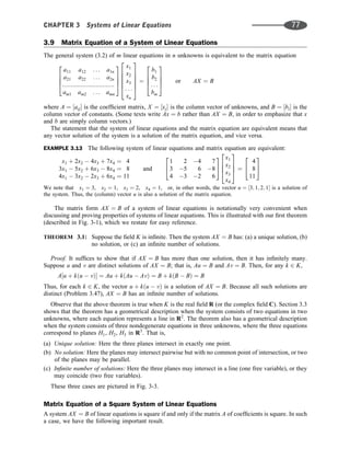
Application to Systems of Linear Equations
Consider a computer algorithm M. Let CðnÞ denote the running time of the algorithm as a function of the
size n of the input data. [The function CðnÞ is sometimes called the time complexity or simply the
complexity of the algorithm M.] Frequently, CðnÞ simply counts the number of multiplications and
divisions executed by M, but does not count the number of additions and subtractions because they take
much less time to execute.
Now consider a square system of linear equations AX ¼ B, where
A ¼ ½aij; X ¼ ½x1; . . . ; xnT
; B ¼ ½b1; . . . ; bnT
and suppose A has an LU factorization. Then the system can be brought into triangular form (in order to
apply back-substitution) by applying Algorithm 3.6 to the augmented matrix M ¼ ½A; B of the system.
The time complexity of Algorithm 3.6 and back-substitution are, respectively,
CðnÞ 1
2 n3
and CðnÞ 1
2 n2
where n is the number of equations.
On the other hand, suppose we already have the factorization A ¼ LU. Then, to triangularize the
system, we need only apply the row operations in the algorithm (retained by the matrix L) to the column
vector B. In this case, the time complexity is
CðnÞ 1
2 n2
Of course, to obtain the factorization A ¼ LU requires the original algorithm where CðnÞ 1
2 n3
. Thus,
nothing may be gained by first finding the LU factorization when a single system is involved. However,
there are situations, illustrated below, where the LU factorization is useful.
Suppose, for a given matrix A, we need to solve the system
AX ¼ B
88 CHAPTER 3 Systems of Linear Equations](https://image.slidesharecdn.com/linearalgebra4thedition-231030053714-df1faee2/85/Linear_Algebra-_4th_Edition-pdf-95-320.jpg)
![Here x1; x2; x4 are the pivot variables and x3 and x5 are the free variables. Recall that the parametric form of
the solution can be obtained from the free-variable form of the solution by simply setting the free variables
equal to parameters, say x3 ¼ a, x5 ¼ b. This process yields
x1 ¼ 21 a 24b; x2 ¼ 7 þ 2a þ 8b; x3 ¼ a; x4 ¼ 3 2b; x5 ¼ b
or u ¼ ð21 a 24b; 7 þ 2a þ 8b; a; 3 2b; bÞ
which is another form of the solution.
Linear Combinations, Homogeneous Systems
3.24. Write v as a linear combination of u1; u2; u3, where
(a) v ¼ ð3; 10; 7Þ and u1 ¼ ð1; 3; 2Þ; u2 ¼ ð1; 4; 2Þ; u3 ¼ ð2; 8; 1Þ;
(b) v ¼ ð2; 7; 10Þ and u1 ¼ ð1; 2; 3Þ, u2 ¼ ð1; 3; 5Þ, u3 ¼ ð1; 5; 9Þ;
(c) v ¼ ð1; 5; 4Þ and u1 ¼ ð1; 3; 2Þ, u2 ¼ ð2; 7; 1Þ, u3 ¼ ð1; 6; 7Þ.
Find the equivalent system of linear equations by writing v ¼ xu1 þ yu2 þ zu3. Alternatively, use the
augmented matrix M of the equivalent system, where M ¼ ½u1; u2; u3; v. (Here u1; u2; u3; v are the columns
of M.)
(a) The vector equation v ¼ xu1 þ yu2 þ zu3 for the given vectors is as follows:
3
10
7
2
4
3
5 ¼ x
1
3
2
2
4
3
5 þ y
1
4
2
2
4
3
5 þ z
2
8
1
2
4
3
5 ¼
x þ y þ 2z
3x þ 4y þ 8z
2x þ 2y þ z
2
4
3
5
Form the equivalent system of linear equations by setting corresponding entries equal to each other, and
then reduce the system to echelon form:
x þ y þ 2z ¼ 3
3x þ 4y þ 8z ¼ 10
2x þ 2y þ z ¼ 7
or
x þ y þ 2z ¼ 3
y þ 2z ¼ 1
4y þ 5z ¼ 13
or
x þ y þ 2z ¼ 3
y þ 2z ¼ 1
3z ¼ 9
The system is in triangular form. Back-substitution yields the unique solution x ¼ 2, y ¼ 7, z ¼ 3.
Thus, v ¼ 2u1 þ 7u2 3u3.
Alternatively, form the augmented matrix M ¼ [u1; u2; u3; v] of the equivalent system, and reduce
M to echelon form:
M ¼
1 1 2 3
3 4 8 10
2 2 1 7
2
4
3
5
1 1 2 3
0 1 2 1
0 4 5 13
2
4
3
5
1 1 2 3
0 1 2 1
0 0 3 9
2
4
3
5
The last matrix corresponds to a triangular system that has a unique solution. Back-substitution yields
the solution x ¼ 2, y ¼ 7, z ¼ 3. Thus, v ¼ 2u1 þ 7u2 3u3.
(b) Form the augmented matrix M ¼ ½u1; u2; u3; v of the equivalent system, and reduce M to the echelon
form:
M ¼
1 1 1 2
2 3 5 7
3 5 9 10
2
4
3
5
1 1 1 2
0 1 3 3
0 2 6 4
2
4
3
5
1 1 1 2
0 1 3 3
0 0 0 2
2
4
3
5
The third row corresponds to the degenerate equation 0x þ 0y þ 0z ¼ 2, which has no solution. Thus,
the system also has no solution, and v cannot be written as a linear combination of u1; u2; u3.
(c) Form the augmented matrix M ¼ ½u1; u2; u3; v of the equivalent system, and reduce M to echelon form:
M ¼
1 2 1 1
3 7 6 5
2 1 7 4
2
4
3
5
1 2 1 1
0 1 3 2
0 3 9 6
2
4
3
5
1 2 1 1
0 1 3 2
0 0 0 0
2
4
3
5
98 CHAPTER 3 Systems of Linear Equations](https://image.slidesharecdn.com/linearalgebra4thedition-231030053714-df1faee2/85/Linear_Algebra-_4th_Edition-pdf-105-320.jpg)
![augmented matrix M, because the last column of the augmented matrix M is a zero column, and it will
remain a zero column during any row-reduction process.
Reduce the coefficient matrix A to echelon form, obtaining
A ¼
1 2 3 2 4
2 4 8 1 9
3 6 13 4 14
2
4
3
5
1 2 3 2 4
0 0 2 5 1
0 0 4 10 2
2
4
3
5 1 2 3 2 4
0 0 2 5 1
(The third row of the second matrix is deleted, because it is a multiple of the second row and will result in a
zero row.) We can now proceed in one of two ways.
(a) Write down the corresponding homogeneous system in echelon form:
x1 þ 2x2 þ 3x3 2x4 þ 4x5 ¼ 0
2x3 þ 5x4 þ x5 ¼ 0
The system in echelon form has three free variables, x2; x4; x5, so dim W ¼ 3. A basis ½u1; u2; u3 for W
may be obtained as follows:
(1) Set x2 ¼ 1, x4 ¼ 0, x5 ¼ 0. Back-substitution yields x3 ¼ 0, and then x1 ¼ 2. Thus,
u1 ¼ ð2; 1; 0; 0; 0Þ.
(2) Set x2 ¼ 0, x4 ¼ 1, x5 ¼ 0. Back-substitution yields x3 ¼ 5
2, and then x1 ¼ 19
2 . Thus,
u2 ¼ ð19
2 ; 0; 5
2 ; 1; 0Þ.
(3) Set x2 ¼ 0, x4 ¼ 0, x5 ¼ 1. Back-substitution yields x3 ¼ 1
2, and then x1 ¼ 5
2. Thus,
u3 ¼ ð 5
2, 0, 1
2 ; 0; 1Þ.
[One could avoid fractions in the basis by choosing x4 ¼ 2 in (2) and x5 ¼ 2 in (3), which yields
multiples of u2 and u3.] The parametric form of the general solution is obtained from the following
linear combination of the basis vectors using parameters a; b; c:
au1 þ bu2 þ cu3 ¼ ð2a þ 19
2 b 5
2 c; a; 5
2 b 1
2 c; b; cÞ
(b) Reduce the echelon form of A to row canonical form:
A
1 2 3 2 4
0 0 1 5
2
1
2
#
1 2 3 19
2
5
2
0 0 1 5
2
1
2
#
Write down the corresponding free-variable solution:
x1 ¼ 2x2 þ
19
2
x4
5
2
x5
x3 ¼
5
2
x4
1
2
x5
Using these equations for the pivot variables x1 and x3, repeat the above process to obtain a basis ½u1; u2; u3
for W. That is, set x2 ¼ 1, x4 ¼ 0, x5 ¼ 0 to get u1; set x2 ¼ 0, x4 ¼ 1, x5 ¼ 0 to get u2; and set x2 ¼ 0,
x4 ¼ 0, x5 ¼ 1 to get u3.
3.28. Prove Theorem 3.15. Let v0 be a particular solution of AX ¼ B, and let W be the general solution
of AX ¼ 0. Then U ¼ v0 þ W ¼ fv0 þ w : w 2 Wg is the general solution of AX ¼ B.
Let w be a solution of AX ¼ 0. Then
Aðv0 þ wÞ ¼ Av0 þ Aw ¼ B þ 0 ¼ B
Thus, the sum v0 þ w is a solution of AX ¼ B. On the other hand, suppose v is also a solution of AX ¼ B.
Then
Aðv v0Þ ¼ Av Av0 ¼ B B ¼ 0
Therefore, v v0 belongs to W. Because v ¼ v0 þ ðv v0Þ, we find that any solution of AX ¼ B can be
obtained by adding a solution of AX ¼ 0 to a solution of AX ¼ B. Thus, the theorem is proved.
100 CHAPTER 3 Systems of Linear Equations](https://image.slidesharecdn.com/linearalgebra4thedition-231030053714-df1faee2/85/Linear_Algebra-_4th_Edition-pdf-107-320.jpg)
![(b) (1) We have
B ¼
1 2 3
0 1 4
0 0 1
2
4
3
5
1 2 0
0 1 0
0 0 1
2
4
3
5
1 0 0
0 1 0
0 0 1
2
4
3
5 ¼ I
where the row operations are, respectively,
‘‘Replace R2 by 4R3 þ R2; ’’ ‘‘Replace R1 by 3R3 þ R1; ’’ ‘‘Replace R1 by 2R2 þ R1’’
(2) Inverse operations:
‘‘Replace R2 by 4R3 þ R2; ’’ ‘‘Replace R1 by 3R3 þ R1; ’’ ‘‘Replace R1 by 2R2 þ R1’’
(3) B ¼
1 0 0
0 1 4
0 0 1
2
4
3
5
1 0 3
0 1 0
0 0 1
2
4
3
5
1 2 0
0 1 0
0 0 1
2
4
3
5
(c) (1) First row reduce C to echelon form. We have
C ¼
1 1 2
2 3 8
3 1 2
2
4
3
5
1 1 2
0 1 4
0 2 8
2
4
3
5
1 1 2
0 1 4
0 0 0
2
4
3
5
In echelon form, C has a zero row. ‘‘STOP.’’ The matrix C cannot be row reduced to the identity
matrix I, and C cannot be written as a product of elementary matrices. (We note, in particular, that
C has no inverse.)
3.32. Find the inverse of (a) A ¼
1 2 4
1 1 5
2 7 3
2
4
3
5; (b) B ¼
1 3 4
1 5 1
3 13 6
2
4
3
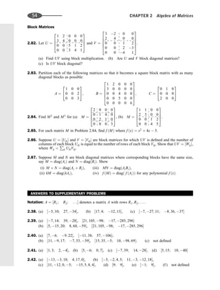
5.
(a) Form the matrix M ¼ [A; I] and row reduce M to echelon form:
M ¼
1 2 4 1 0 0
1 1 5 0 1 0
2 7 3 0 0 1
2
6
4
3
7
5
1 2 4 1 0 0
0 1 1 1 1 0
0 3 5 2 0 1
2
6
4
3
7
5
1 2 4 1 0 0
0 1 1 1 1 0
0 0 2 5 3 1
2
6
4
3
7
5
In echelon form, the left half of M is in triangular form; hence, A has an inverse. Further reduce M to
row canonical form:
M
1 2 0 9 6 2
0 1 0 7
2
5
2 1
2
0 0 1 5
2 3
2
1
2
2
6
6
4
3
7
7
5
1 0 0 16 11 3
0 1 0 7
2
5
2 1
2
0 0 1 5
2 3
2
1
2
2
6
6
4
3
7
7
5
The final matrix has the form ½I; A1
; that is, A1
is the right half of the last matrix. Thus,
A1
¼
16 11 3
7
2
5
2 1
2
5
2 3
2
1
2
2
6
6
4
3
7
7
5
(b) Form the matrix M ¼ ½B; I and row reduce M to echelon form:
M ¼
1 3 4 1 0 0
1 5 1 0 1 0
3 13 6 0 0 1
2
4
3
5
1 3 4 1 0 0
0 2 3 1 1 0
0 4 6 3 0 1
2
4
3
5
1 3 4 1 0 0
0 2 3 1 1 0
0 0 0 1 2 1
2
4
3
5
In echelon form, M has a zero row in its left half; that is, B is not row reducible to triangular form.
Accordingly, B has no inverse.
102 CHAPTER 3 Systems of Linear Equations](https://image.slidesharecdn.com/linearalgebra4thedition-231030053714-df1faee2/85/Linear_Algebra-_4th_Edition-pdf-109-320.jpg)
![[A1] ðu þ vÞ þ w ¼ u þ ðv þ wÞ
[A2] There is a vector in V, denoted by 0 and called the zero vector, such that, for any
u 2 V;
u þ 0 ¼ 0 þ u ¼ u
[A3] For each u 2 V; there is a vector in V, denoted by u, and called the negative of u,
such that
u þ ðuÞ ¼ ðuÞ þ u ¼ 0.
[A4] u þ v ¼ v þ u.
[M1] kðu þ vÞ ¼ ku þ kv, for any scalar k 2 K:
[M2] ða þ bÞu ¼ au þ bu; for any scalars a; b 2 K.
[M3] ðabÞu ¼ aðbuÞ; for any scalars a; b 2 K.
[M4] 1u ¼ u, for the unit scalar 1 2 K.
The above axioms naturally split into two sets (as indicated by the labeling of the axioms). The first
four are concerned only with the additive structure of V and can be summarized by saying V is a
commutative group under addition. This means
(a) Any sum v1 þ v2 þ þ vm of vectors requires no parentheses and does not depend on the order of
the summands.
(b) The zero vector 0 is unique, and the negative u of a vector u is unique.
(c) (Cancellation Law) If u þ w ¼ v þ w, then u ¼ v.
Also, subtraction in V is defined by u v ¼ u þ ðvÞ, where v is the unique negative of v.
On the other hand, the remaining four axioms are concerned with the ‘‘action’’ of the field K of scalars
on the vector space V. Using these additional axioms, we prove (Problem 4.2) the following simple
properties of a vector space.
THEOREM 4.1: Let V be a vector space over a field K.
(i) For any scalar k 2 K and 0 2 V; k0 ¼ 0.
(ii) For 0 2 K and any vector u 2 V; 0u ¼ 0.
(iii) If ku ¼ 0, where k 2 K and u 2 V, then k ¼ 0 or u ¼ 0.
(iv) For any k 2 K and any u 2 V; ðkÞu ¼ kðuÞ ¼ ku.
4.3 Examples of Vector Spaces
This section lists important examples of vector spaces that will be used throughout the text.
Space Kn
Let K be an arbitrary field. The notation Kn
is frequently used to denote the set of all n-tuples of elements
in K. Here Kn
is a vector space over K using the following operations:
(i) Vector Addition: ða1; a2; . . . ; anÞ þ ðb1; b2; . . . ; bnÞ ¼ ða1 þ b1; a2 þ b2; . . . ; an þ bnÞ
(ii) Scalar Multiplication: kða1; a2; . . . ; anÞ ¼ ðka1; ka2; . . . ; kanÞ
The zero vector in Kn
is the n-tuple of zeros,
0 ¼ ð0; 0; . . . ; 0Þ
and the negative of a vector is defined by
ða1; a2; . . . ; anÞ ¼ ða1; a2; . . . ; anÞ
Observe that these are the same as the operations defined for Rn
in Chapter 1. The proof that Kn
is a
vector space is identical to the proof of Theorem 1.1, which we now regard as stating that Rn
with the
operations defined there is a vector space over R.
CHAPTER 4 Vector Spaces 113](https://image.slidesharecdn.com/linearalgebra4thedition-231030053714-df1faee2/85/Linear_Algebra-_4th_Edition-pdf-120-320.jpg)
![Polynomial Space PðtÞ
Let PðtÞ denote the set of all polynomials of the form
pðtÞ ¼ a0 þ a1t þ a2t2
þ þ asts
ðs ¼ 1; 2; . . .Þ
where the coefficients ai belong to a field K. Then PðtÞ is a vector space over K using the following operations:
(i) Vector Addition: Here pðtÞ þ qðtÞ in PðtÞ is the usual operation of addition of polynomials.
(ii) Scalar Multiplication: Here kpðtÞ in PðtÞ is the usual operation of the product of a scalar k and a
polynomial pðtÞ.
The zero polynomial 0 is the zero vector in PðtÞ.
Polynomial Space PnðtÞ
Let PnðtÞ denote the set of all polynomials pðtÞ over a field K, where the degree of pðtÞ is less than or
equal to n; that is,
pðtÞ ¼ a0 þ a1t þ a2t2
þ þ asts
where s n. Then PnðtÞ is a vector space over K with respect to the usual operations of addition of
polynomials and of multiplication of a polynomial by a constant (just like the vector space PðtÞ above).
We include the zero polynomial 0 as an element of PnðtÞ, even though its degree is undefined.
Matrix Space Mm;n
The notation Mm;n, or simply M; will be used to denote the set of all m n matrices with entries in a field
K. Then Mm;n is a vector space over K with respect to the usual operations of matrix addition and scalar
multiplication of matrices, as indicated by Theorem 2.1.
Function Space FðXÞ
Let X be a nonempty set and let K be an arbitrary field. Let FðXÞ denote the set of all functions of X into
K. [Note that FðXÞ is nonempty, because X is nonempty.] Then FðXÞ is a vector space over K with
respect to the following operations:
(i) Vector Addition: The sum of two functions f and g in FðXÞ is the function f þ g in FðXÞ defined by
ð f þ gÞðxÞ ¼ f ðxÞ þ gðxÞ 8x 2 X
(ii) Scalar Multiplication: The product of a scalar k 2 K and a function f in FðXÞ is the function kf in
FðXÞ defined by
ðkf ÞðxÞ ¼ kf ðxÞ 8x 2 X
The zero vector in FðXÞ is the zero function 0, which maps every x 2 X into the zero element 0 2 K;
0ðxÞ ¼ 0 8x 2 X
Also, for any function f in FðXÞ, negative of f is the function f in FðXÞ defined by
ðf ÞðxÞ ¼ f ðxÞ 8x 2 X
Fields and Subfields
Suppose a field E is an extension of a field K; that is, suppose E is a field that contains K as a subfield.
Then E may be viewed as a vector space over K using the following operations:
(i) Vector Addition: Here u þ v in E is the usual addition in E.
(ii) Scalar Multiplication: Here ku in E, where k 2 K and u 2 E, is the usual product of k and u as
elements of E.
That is, the eight axioms of a vector space are satisfied by E and its subfield K with respect to the above
two operations.
114 CHAPTER 4 Vector Spaces](https://image.slidesharecdn.com/linearalgebra4thedition-231030053714-df1faee2/85/Linear_Algebra-_4th_Edition-pdf-121-320.jpg)
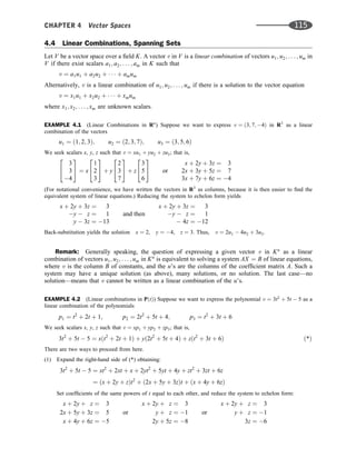
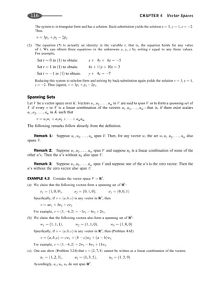
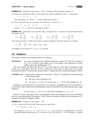
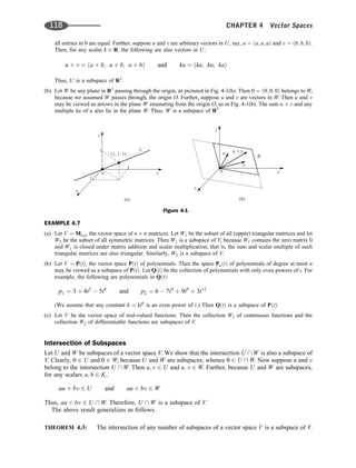
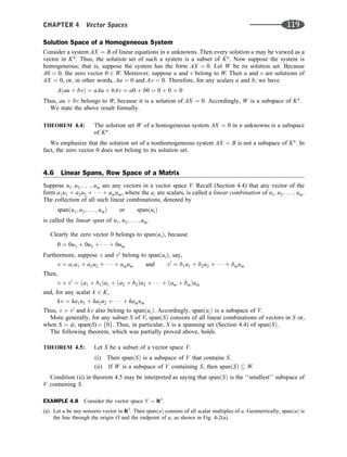
![(b) Let u and v be vectors in R3
that are not multiples of each other. Then spanðu; vÞ is the plane through the origin
O and the endpoints of u and v as shown in Fig. 4-2(b).
(c) Consider the vectors e1 ¼ ð1; 0; 0Þ, e2 ¼ ð0; 1; 0Þ, e3 ¼ ð0; 0; 1Þ in R3
. Recall [Example 4.1(a)] that every vector
in R3
is a linear combination of e1, e2, e3. That is, e1, e2, e3 form a spanning set of R3
. Accordingly,
spanðe1; e2; e3Þ ¼ R3
.
Row Space of a Matrix
Let A ¼ ½aij be an arbitrary m n matrix over a field K. The rows of A,
R1 ¼ ða11; a12; . . . ; a1nÞ; R2 ¼ ða21; a22; . . . ; a2nÞ; . . . ; Rm ¼ ðam1; am2; . . . ; amnÞ
may be viewed as vectors in Kn
; hence, they span a subspace of Kn
called the row space of A and denoted
by rowsp(A). That is,
rowspðAÞ ¼ spanðR1; R2; . . . ; RmÞ
Analagously, the columns of A may be viewed as vectors in Km
called the column space of A and denoted
by colsp(A). Observe that colspðAÞ ¼ rowspðAT
Þ.
Recall that matrices A and B are row equivalent, written A B, if B can be obtained from A by a
sequence of elementary row operations. Now suppose M is the matrix obtained by applying one of the
following elementary row operations on a matrix A:
ð1Þ Interchange Ri and Rj; ð2Þ Replace Ri by kRi; ð3Þ Replace Rj by kRi þ Rj
Then each row of M is a row of A or a linear combination of rows of A. Hence, the row space of M is
contained in the row space of A. On the other hand, we can apply the inverse elementary row operation on
M to obtain A; hence, the row space of A is contained in the row space of M. Accordingly, A and M have
the same row space. This will be true each time we apply an elementary row operation. Thus, we have
proved the following theorem.
THEOREM 4.6: Row equivalent matrices have the same row space.
We are now able to prove (Problems 4.45–4.47) basic results on row equivalence (which first
appeared as Theorems 3.7 and 3.8 in Chapter 3).
THEOREM 4.7: Suppose A ¼ ½aij and B ¼ ½bij are row equivalent echelon matrices with respective
pivot entries
a1j1
; a2j2
; . . . ; arjr
and b1k1
; b2k2
; . . . ; bsks
Then A and B have the same number of nonzero rows—that is, r ¼ s—and their
pivot entries are in the same positions—that is, j1 ¼ k1; j2 ¼ k2; . . . ; jr ¼ kr.
THEOREM 4.8: Suppose A and B are row canonical matrices. Then A and B have the same row space
if and only if they have the same nonzero rows.
0
(a)
u
Figure 4-2
0
(b)
u
120 CHAPTER 4 Vector Spaces](https://image.slidesharecdn.com/linearalgebra4thedition-231030053714-df1faee2/85/Linear_Algebra-_4th_Edition-pdf-127-320.jpg)
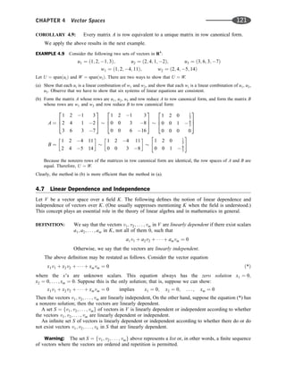
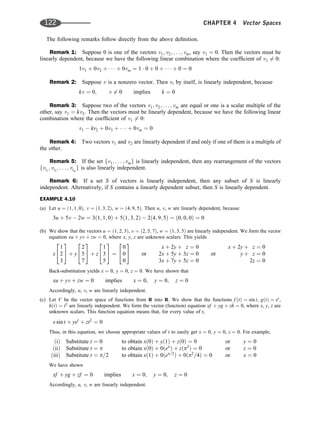
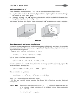
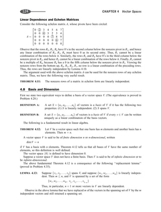
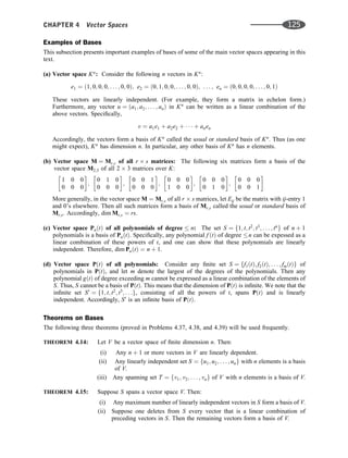
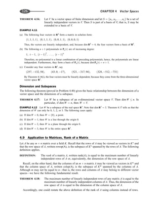
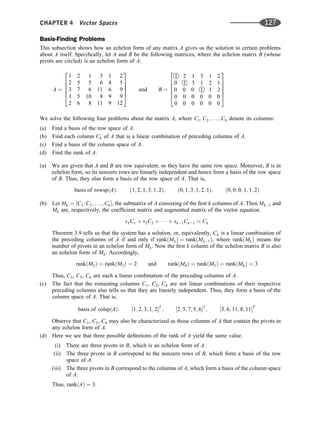
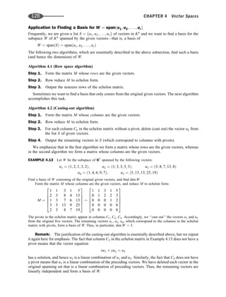
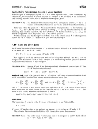
![EXAMPLE 4.15 Consider the vector space V ¼ R3
:
(a) Let U be the xy-plane and let W be the yz-plane; that is,
U ¼ fða; b; 0Þ : a; b 2 Rg and W ¼ fð0; b; cÞ : b; c 2 Rg
Then R3
¼ U þ W, because every vector in R3
is the sum of a vector in U and a vector in W. However, R3
is not
the direct sum of U and W, because such sums are not unique. For example,
ð3; 5; 7Þ ¼ ð3; 1; 0Þ þ ð0; 4; 7Þ and also ð3; 5; 7Þ ¼ ð3; 4; 0Þ þ ð0; 9; 7Þ
(b) Let U be the xy-plane and let W be the z-axis; that is,
U ¼ fða; b; 0Þ : a; b 2 Rg and W ¼ fð0; 0; cÞ : c 2 Rg
Now any vector ða; b; cÞ 2 R3
can be written as the sum of a vector in U and a vector in V in one and only one
way:
ða; b; cÞ ¼ ða; b; 0Þ þ ð0; 0; cÞ
Accordingly, R3
is the direct sum of U and W; that is, R3
¼ U W.
General Direct Sums
The notion of a direct sum is extended to more than one factor in the obvious way. That is, V is the direct
sum of subspaces W1; W2; . . . ; Wr, written
V ¼ W1 W2 Wr
if every vector v 2 V can be written in one and only one way as
v ¼ w1 þ w2 þ þ wr
where w1 2 W1; w2 2 W2; . . . ; wr 2 Wr.
The following theorems hold.
THEOREM 4.22: Suppose V ¼ W1 W2 Wr. Also, for each k, suppose Sk is a linearly
independent subset of Wk. Then
(a) The union S ¼
S
k Sk is linearly independent in V.
(b) If each Sk is a basis of Wk, then
S
k Sk is a basis of V.
(c) dim V ¼ dim W1 þ dim W2 þ þ dim Wr.
THEOREM 4.23: Suppose V ¼ W1 þ W2 þ þ Wr and dim V ¼
P
k dim Wk. Then
V ¼ W1 W2 Wr:
4.11 Coordinates
Let V be an n-dimensional vector space over K with basis S ¼ fu1; u2; . . . ; ung. Then any vector v 2 V
can be expressed uniquely as a linear combination of the basis vectors in S, say
v ¼ a1u1 þ a2u2 þ þ anun
These n scalars a1; a2; . . . ; an are called the coordinates of v relative to the basis S, and they form a vector
[a1; a2; . . . ; an] in Kn
called the coordinate vector of v relative to S. We denote this vector by ½vS, or
simply ½v; when S is understood. Thus,
½vS ¼ ½a1; a2; . . . ; an
For notational convenience, brackets ½. . ., rather than parentheses ð. . .Þ, are used to denote the coordinate
vector.
130 CHAPTER 4 Vector Spaces](https://image.slidesharecdn.com/linearalgebra4thedition-231030053714-df1faee2/85/Linear_Algebra-_4th_Edition-pdf-137-320.jpg)
![Remark: The above n scalars a1; a2; . . . ; an also form the coordinate column vector
½a1; a2; . . . ; anT
of v relative to S. The choice of the column vector rather than the row vector to
represent v depends on the context in which it is used. The use of such column vectors will become clear
later in Chapter 6.
EXAMPLE 4.16 Consider the vector space P2ðtÞ of polynomials of degree 2. The polynomials
p1 ¼ t þ 1; p2 ¼ t 1; p3 ¼ ðt 1Þ2
¼ t2
2t þ 1
form a basis S of P2ðtÞ. The coordinate vector [v] of v ¼ 2t2
5t þ 9 relative to S is obtained as follows.
Set v ¼ xp1 þ yp2 þ zp3 using unknown scalars x, y, z, and simplify:
2t2
5t þ 9 ¼ xðt þ 1Þ þ yðt 1Þ þ zðt2
2t þ 1Þ
¼ xt þ x þ yt y þ zt2
2zt þ z
¼ zt2
þ ðx þ y 2zÞt þ ðx y þ zÞ
Then set the coefficients of the same powers of t equal to each other to obtain the system
z ¼ 2; x þ y 2z ¼ 5; x y þ z ¼ 9
The solution of the system is x ¼ 3, y ¼ 4, z ¼ 2. Thus,
v ¼ 3p1 4p2 þ 2p3; and hence; ½v ¼ ½3; 4; 2
EXAMPLE 4.17 Consider real space R3
. The following vectors form a basis S of R3
:
u1 ¼ ð1; 1; 0Þ; u2 ¼ ð1; 1; 0Þ; u3 ¼ ð0; 1; 1Þ
The coordinates of v ¼ ð5; 3; 4Þ relative to the basis S are obtained as follows.
Set v ¼ xv1 þ yv2 þ zv3; that is, set v as a linear combination of the basis vectors using unknown scalars x, y, z.
This yields
5
3
4
2
4
3
5 ¼ x
1
1
0
2
4
3
5 þ y
1
1
0
2
4
3
5 þ z
0
1
1
2
4
3
5
The equivalent system of linear equations is as follows:
x þ y ¼ 5; x þ y þ z ¼ 3; z ¼ 4
The solution of the system is x ¼ 3, y ¼ 2, z ¼ 4. Thus,
v ¼ 3u1 þ 2u2 þ 4u3; and so ½vs ¼ ½3; 2; 4
Remark 1: There is a geometrical interpretation of the coordinates of a vector v relative to a basis
S for the real space Rn
, which we illustrate using the basis S of R3
in Example 4.17. First consider the
space R3
with the usual x, y, z axes. Then the basis vectors determine a new coordinate system of R3
, say
with x0
, y0
, z0
axes, as shown in Fig. 4-4. That is,
(1) The x0
-axis is in the direction of u1 with unit length ku1k.
(2) The y0
-axis is in the direction of u2 with unit length ku2k.
(3) The z0
-axis is in the direction of u3 with unit length ku3k.
Then each vector v ¼ ða; b; cÞ or, equivalently, the point Pða; b; cÞ in R3
will have new coordinates with
respect to the new x0
, y0
, z0
axes. These new coordinates are precisely ½vS, the coordinates of v with
respect to the basis S. Thus, as shown in Example 4.17, the coordinates of the point Pð5; 3; 4Þ with the
new axes form the vector [3, 2, 4].
Remark 2: Consider the usual basis E ¼ fe1; e2; . . . ; eng of Kn
defined by
e1 ¼ ð1; 0; 0; . . . ; 0; 0Þ; e2 ¼ ð0; 1; 0; . . . ; 0; 0Þ; . . . ; en ¼ ð0; 0; 0; . . . ; 0; 1Þ
CHAPTER 4 Vector Spaces 131](https://image.slidesharecdn.com/linearalgebra4thedition-231030053714-df1faee2/85/Linear_Algebra-_4th_Edition-pdf-138-320.jpg)
![Let v ¼ ða1; a2; . . . ; anÞ be any vector in Kn
. Then one can easily show that
v ¼ a1e1 þ a2e2 þ þ anen; and so ½vE ¼ ½a1; a2; . . . ; an
That is, the coordinate vector ½vE of any vector v relative to the usual basis E of Kn
is identical to the
original vector v.
Isomorphism of V and Kn
Let V be a vector space of dimension n over K, and suppose S ¼ fu1; u2; . . . ; ung is a basis of V. Then
each vector v 2 V corresponds to a unique n-tuple ½vS in Kn
. On the other hand, each n-tuple
[c1; c2; . . . ; cn] in Kn
corresponds to a unique vector c1u1 þ c2u2 þ þ cnun in V. Thus, the basis S
induces a one-to-one correspondence between V and Kn
. Furthermore, suppose
v ¼ a1u1 þ a2u2 þ þ anun and w ¼ b1u1 þ b2u2 þ þ bnun
Then
v þ w ¼ ða1 þ b1Þu1 þ ða2 þ b2Þu2 þ þ ðan þ bnÞun
kv ¼ ðka1Þu1 þ ðka2Þu2 þ þ ðkanÞun
where k is a scalar. Accordingly,
½v þ wS ¼ ½a1 þ b1; . . . ; an þ bn ¼ ½a1; . . . ; an þ ½b1; . . . ; bn ¼ ½vS þ ½wS
½kvS ¼ ½ka1; ka2; . . . ; kan ¼ k½a1; a2; . . . ; an ¼ k½vS
Thus, the above one-to-one correspondence between V and Kn
preserves the vector space operations of
vector addition and scalar multiplication. We then say that V and Kn
are isomorphic, written
V ffi Kn
We state this result formally.
Figure 4-4
132 CHAPTER 4 Vector Spaces](https://image.slidesharecdn.com/linearalgebra4thedition-231030053714-df1faee2/85/Linear_Algebra-_4th_Edition-pdf-139-320.jpg)
![THEOREM 4.24: Let V be an n-dimensional vector space over a field K. Then V and Kn
are
isomorphic.
The next example gives a practical application of the above result.
EXAMPLE 4.18 Suppose we want to determine whether or not the following matrices in V ¼ M2;3 are linearly
dependent:
A ¼
1 2 3
4 0 1
; B ¼
1 3 4
6 5 4
; C ¼
3 8 11
16 10 9
The coordinate vectors of the matrices in the usual basis of M2;3 are as follows:
½A ¼ ½1; 2; 3; 4; 0; 1; ½B ¼ ½1; 3; 4; 6; 5; 4; ½C ¼ ½3; 8; 11; 16; 10; 9
Form the matrix M whose rows are the above coordinate vectors and reduce M to an echelon form:
M ¼
1 2 3 4 0 1
1 3 4 6 5 4
3 8 11 16 10 9
2
4
3
5
1 2 3 4 0 1
0 1 1 2 5 3
0 2 2 4 10 6
2
4
3
5
1 2 3 4 0 1
0 1 1 2 5 3
0 0 0 0 0 0
2
4
3
5
Because the echelon matrix has only two nonzero rows, the coordinate vectors [A], [B], [C] span a subspace of
dimension 2 and so are linearly dependent. Accordingly, the original matrices A, B, C are linearly dependent.
SOLVED PROBLEMS
Vector Spaces, Linear Combinations
4.1. Suppose u and v belong to a vector space V. Simplify each of the following expressions:
(a) E1 ¼ 3ð2u 4vÞ þ 5u þ 7v, (c) E3 ¼ 2uv þ 3ð2u þ 4vÞ
(b) E2 ¼ 3u 6ð3u 5vÞ þ 7u, (d) E4 ¼ 5u
3
v
þ 5u
Multiply out and collect terms:
(a) E1 ¼ 6u 12v þ 5u þ 7v ¼ 11u 5v
(b) E2 ¼ 3u 18u þ 30v þ 7u ¼ 8u þ 30v
(c) E3 is not defined because the product uv of vectors is not defined.
(d) E4 is not defined because division by a vector is not defined.
4.2. Prove Theorem 4.1: Let V be a vector space over a field K.
(i) k0 ¼ 0. (ii) 0u ¼ 0. (iii) If ku ¼ 0, then k ¼ 0 or u ¼ 0. (iv) ðkÞu ¼ kðuÞ ¼ ku.
(i) By Axiom [A2] with u ¼ 0, we have 0 þ 0 ¼ 0. Hence, by Axiom [M1], we have
k0 ¼ kð0 þ 0Þ ¼ k0 þ k0
Adding k0 to both sides gives the desired result.
(ii) For scalars, 0 þ 0 ¼ 0. Hence, by Axiom [M2], we have
0u ¼ ð0 þ 0Þu ¼ 0u þ 0u
Adding 0u to both sides gives the desired result.
(iii) Suppose ku ¼ 0 and k 6¼ 0. Then there exists a scalar k1
such that k1
k ¼ 1. Thus,
u ¼ 1u ¼ ðk1
kÞu ¼ k1
ðkuÞ ¼ k1
0 ¼ 0
(iv) Using u þ ðuÞ ¼ 0 and k þ ðkÞ ¼ 0 yields
0 ¼ k0 ¼ k½u þ ðuÞ ¼ ku þ kðuÞ and 0 ¼ 0u ¼ ½k þ ðkÞu ¼ ku þ ðkÞu
Adding ku to both sides of the first equation gives ku ¼ kðuÞ; and adding ku to both sides of the
second equation gives ku ¼ ðkÞu. Thus, ðkÞu ¼ kðuÞ ¼ ku.
CHAPTER 4 Vector Spaces 133](https://image.slidesharecdn.com/linearalgebra4thedition-231030053714-df1faee2/85/Linear_Algebra-_4th_Edition-pdf-140-320.jpg)
![4.3. Show that (a) kðu vÞ ¼ ku kv, (b) u þ u ¼ 2u.
(a) Using the definition of subtraction, that u v ¼ u þ ðvÞ, and Theorem 4.1(iv), that kðvÞ ¼ kv, we
have
kðu vÞ ¼ k½u þ ðvÞ ¼ ku þ kðvÞ ¼ ku þ ðkvÞ ¼ ku kv
(b) Using Axiom [M4] and then Axiom [M2], we have
u þ u ¼ 1u þ 1u ¼ ð1 þ 1Þu ¼ 2u
4.4. Express v ¼ ð1; 2; 5Þ in R3
as a linear combination of the vectors
u1 ¼ ð1; 1; 1Þ; u2 ¼ ð1; 2; 3Þ; u3 ¼ ð2; 1; 1Þ
We seek scalars x, y, z, as yet unknown, such that v ¼ xu1 þ yu2 þ zu3. Thus, we require
1
2
5
2
4
3
5 ¼ x
1
1
1
2
4
3
5 þ y
1
2
3
2
4
3
5 þ z
2
1
1
2
4
3
5 or
x þ y þ 2z ¼ 1
x þ 2y z ¼ 2
x þ 3y þ z ¼ 5
(For notational convenience, we write the vectors in R3
as columns, because it is then easier to find the
equivalent system of linear equations.) Reducing the system to echelon form yields the triangular system
x þ y þ 2z ¼ 1; y 3z ¼ 3; 5z ¼ 10
The system is consistent and has a solution. Solving by back-substitution yields the solution x ¼ 6, y ¼ 3,
z ¼ 2. Thus, v ¼ 6u1 þ 3u2 þ 2u3.
Alternatively, write down the augmented matrix M of the equivalent system of linear equations, where
u1, u2, u3 are the first three columns of M and v is the last column, and then reduce M to echelon form:
M ¼
1 1 2 1
1 2 1 2
1 3 1 5
2
4
3
5
1 1 2 1
0 1 3 3
0 2 1 4
2
4
3
5
1 1 2 1
0 1 3 3
0 0 5 10
2
4
3
5
The last matrix corresponds to a triangular system, which has a solution. Solving the triangular system by
back-substitution yields the solution x ¼ 6, y ¼ 3, z ¼ 2. Thus, v ¼ 6u1 þ 3u2 þ 2u3.
4.5. Express v ¼ ð2; 5; 3Þ in R3
as a linear combination of the vectors
u1 ¼ ð1; 3; 2Þ; u2 ¼ ð2; 4; 1Þ; u3 ¼ ð1; 5; 7Þ
We seek scalars x, y, z, as yet unknown, such that v ¼ xu1 þ yu2 þ zu3. Thus, we require
2
5
3
2
4
3
5 ¼ x
1
3
2
2
4
3
5 þ y
2
4
1
2
4
3
5 þ z
1
5
7
2
4
3
5 or
x þ 2y þ z ¼ 2
3x 4y 5z ¼ 5
2x y þ 7z ¼ 3
Reducing the system to echelon form yields the system
x þ 2y þ z ¼ 2; 2y 2z ¼ 1; 0 ¼ 3
The system is inconsistent and so has no solution. Thus, v cannot be written as a linear combination of
u1, u2, u3.
4.6. Express the polynomial v ¼ t2
þ 4t 3 in PðtÞ as a linear combination of the polynomials
p1 ¼ t2
2t þ 5; p2 ¼ 2t2
3t; p3 ¼ t þ 1
Set v as a linear combination of p1, p2, p3 using unknowns x, y, z to obtain
t2
þ 4t 3 ¼ xðt2
2t þ 5Þ þ yð2t2
3tÞ þ zðt þ 1Þ ð*Þ
We can proceed in two ways.
134 CHAPTER 4 Vector Spaces](https://image.slidesharecdn.com/linearalgebra4thedition-231030053714-df1faee2/85/Linear_Algebra-_4th_Edition-pdf-141-320.jpg)
![Method 1. Expand the right side of (*) and express it in terms of powers of t as follows:
t2
þ 4t 3 ¼ xt2
2xt þ 5x þ 2yt2
3yt þ zt þ z
¼ ðx þ 2yÞt2
þ ð2x 3y þ zÞt þ ð5x þ 3zÞ
Set coefficients of the same powers of t equal to each other, and reduce the system to echelon form. This
yields
x þ 2y ¼ 1
2x 3y þ z ¼ 4
5x þ 3z ¼ 3
or
x þ 2y ¼ 1
y þ z ¼ 6
10y þ 3z ¼ 8
or
x þ 2y ¼ 1
y þ z ¼ 6
13z ¼ 52
The system is consistent and has a solution. Solving by back-substitution yields the solution x ¼ 3, y ¼ 2,
z ¼ 4. Thus, v ¼ 3p1 þ 2p2 þ 4p2.
Method 2. The equation (*) is an identity in t; that is, the equation holds for any value of t. Thus, we can
set t equal to any numbers to obtain equations in the unknowns.
(a) Set t ¼ 0 in (*) to obtain the equation 3 ¼ 5x þ z.
(b) Set t ¼ 1 in (*) to obtain the equation 2 ¼ 4x y þ 2z.
(c) Set t ¼ 1 in (*) to obtain the equation 6 ¼ 8x þ 5y.
Solve the system of the three equations to again obtain the solution x ¼ 3, y ¼ 2, z ¼ 4. Thus,
v ¼ 3p1 þ 2p2 þ 4p3.
4.7. Express M as a linear combination of the matrices A, B, C, where
M ¼
4 7
7 9
; and A ¼
1 1
1 1
; B ¼
1 2
3 4
; C ¼
1 1
4 5
Set M as a linear combination of A, B, C using unknown scalars x, y, z; that is, set M ¼ xA þ yB þ zC.
This yields
4 7
7 9
¼ x
1 1
1 1
þ y
1 2
3 4
þ z
1 1
4 5
¼
x þ y þ z x þ 2y þ z
x þ 3y þ 4z x þ 4y þ 5z
Form the equivalent system of equations by setting corresponding entries equal to each other:
x þ y þ z ¼ 4; x þ 2y þ z ¼ 7; x þ 3y þ 4z ¼ 7; x þ 4y þ 5z ¼ 9
Reducing the system to echelon form yields
x þ y þ z ¼ 4; y ¼ 3; 3z ¼ 3; 4z ¼ 4
The last equation drops out. Solving the system by back-substitution yields z ¼ 1, y ¼ 3, x ¼ 2. Thus,
M ¼ 2A þ 3B C.
Subspaces
4.8. Prove Theorem 4.2: W is a subspace of V if the following two conditions hold:
(a) 0 2 W. (b) If u; v 2 W, then u þ v, ku 2 W.
By (a), W is nonempty, and, by (b), the operations of vector addition and scalar multiplication are well
defined for W. Axioms [A1], [A4], [M1], [M2], [M3], [M4] hold in W because the vectors in W belong to V.
Thus, we need only show that [A2] and [A3] also hold in W. Now [A2] holds because the zero vector in V
belongs to W by (a). Finally, if v 2 W, then ð1Þv ¼ v 2 W, and v þ ðvÞ ¼ 0. Thus [A3] holds.
4.9. Let V ¼ R3
. Show that W is not a subspace of V, where
(a) W ¼ fða; b; cÞ : a 0g, (b) W ¼ fða; b; cÞ : a2
þ b2
þ c2
1g.
In each case, show that Theorem 4.2 does not hold.
CHAPTER 4 Vector Spaces 135](https://image.slidesharecdn.com/linearalgebra4thedition-231030053714-df1faee2/85/Linear_Algebra-_4th_Edition-pdf-142-320.jpg)
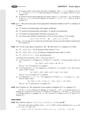
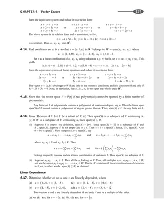
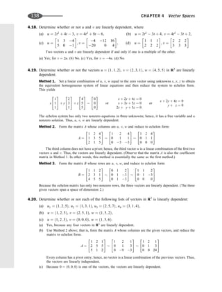
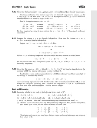
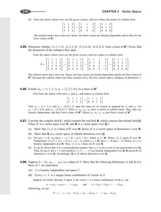
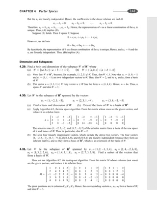
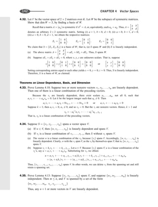
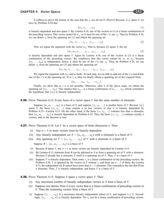
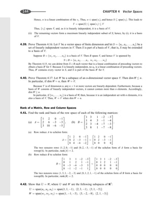
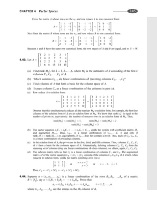
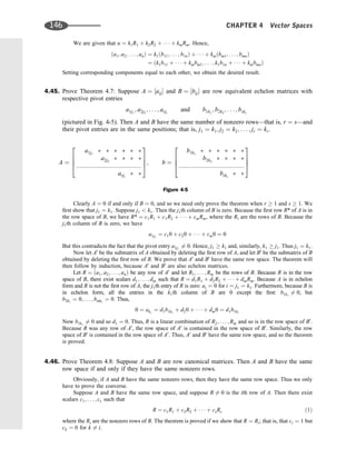
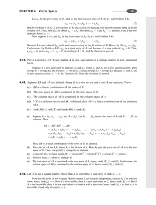
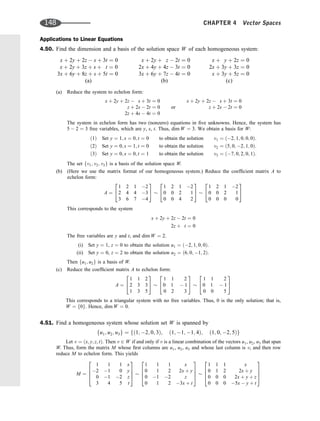
![But fa1; . . . ; amg is linearly independent over K; hence, because the xji 2 K,
x11 ¼ 0; x12 ¼ 0; . . . ; x1m ¼ 0; . . . ; xn1 ¼ 0; xn2 ¼ 0; . . . ; xnm ¼ 0
Accordingly, faivjg is linearly independent over K, and the theorem is proved.
SUPPLEMENTARY PROBLEMS
Vector Spaces
4.71. Suppose u and v belong to a vector space V. Simplify each of the following expressions:
(a) E1 ¼ 4ð5u 6vÞ þ 2ð3u þ vÞ, (c) E3 ¼ 6ð3u þ 2vÞ þ 5u 7v,
(b) E2 ¼ 5ð2u 3vÞ þ 4ð7v þ 8Þ, (d) E4 ¼ 3ð5u þ 2=vÞ:
4.72. Let V be the set of ordered pairs (a; b) of real numbers with addition in V and scalar multiplication on V
defined by
ða; bÞ þ ðc; dÞ ¼ ða þ c; b þ dÞ and kða; bÞ ¼ ðka; 0Þ
Show that V satisfies all the axioms of a vector space except [M4]—that is, except 1u ¼ u. Hence, [M4] is
not a consequence of the other axioms.
4.73. Show that Axiom [A4] of a vector space V (that u þ v ¼ v þ u) can be derived from the other axioms for V.
4.74. Let V be the set of ordered pairs (a; b) of real numbers. Show that V is not a vector space over R with
addition and scalar multiplication defined by
(i) ða; bÞ þ ðc; dÞ ¼ ða þ d; b þ cÞ and kða; bÞ ¼ ðka; kbÞ,
(ii) ða; bÞ þ ðc; dÞ ¼ ða þ c; b þ dÞ and kða; bÞ ¼ ða; bÞ,
(iii) ða; bÞ þ ðc; dÞ ¼ ð0; 0Þ and kða; bÞ ¼ ðka; kbÞ,
(iv) ða; bÞ þ ðc; dÞ ¼ ðac; bdÞ and kða; bÞ ¼ ðka; kbÞ.
4.75. Let V be the set of infinite sequences (a1; a2; . . .) in a field K. Show that V is a vector space over K with
addition and scalar multiplication defined by
ða1; a2; . . .Þ þ ðb1; b2; . . .Þ ¼ ða1 þ b1; a2 þ b2; . . .Þ and kða1; a2; . . .Þ ¼ ðka1; ka2; . . .Þ
4.76. Let U and W be vector spaces over a field K. Let V be the set of ordered pairs (u; w) where u 2 U and
w 2 W. Show that V is a vector space over K with addition in V and scalar multiplication on V defined by
ðu; wÞ þ ðu0
; w0
Þ ¼ ðu þ u0
; w þ w0
Þ and kðu; wÞ ¼ ðku; kwÞ
(This space V is called the external direct product of U and W.)
Subspaces
4.77. Determine whether or not W is a subspace of R3
where W consists of all vectors (a; b; c) in R3
such that
(a) a ¼ 3b, (b) a b c, (c) ab ¼ 0, (d) a þ b þ c ¼ 0, (e) b ¼ a2
, ( f ) a ¼ 2b ¼ 3c.
4.78. Let V be the vector space of n-square matrices over a field K. Show that W is a subspace of V if W consists
of all matrices A ¼ ½aij that are
(a) symmetric (AT
¼ A or aij ¼ aji), (b) (upper) triangular, (c) diagonal, (d) scalar.
4.79. Let AX ¼ B be a nonhomogeneous system of linear equations in n unknowns; that is, B 6¼ 0. Show that the
solution set is not a subspace of Kn
.
4.80. Suppose U and W are subspaces of V for which U [ W is a subspace. Show that U W or W U.
4.81. Let V be the vector space of all functions from the real field R into R. Show that W is a subspace of V
where W consists of all: (a) bounded functions, (b) even functions. [Recall that f : R ! R is bounded if
9M 2 R such that 8x 2 R, we have j f ðxÞj M; and f ðxÞ is even if f ðxÞ ¼ f ðxÞ; 8x 2 R.]
156 CHAPTER 4 Vector Spaces](https://image.slidesharecdn.com/linearalgebra4thedition-231030053714-df1faee2/85/Linear_Algebra-_4th_Edition-pdf-163-320.jpg)
![4.82. Let V be the vector space (Problem 4.75) of infinite sequences (a1; a2; . . .) in a field K. Show that W is a
subspace of V if W consists of all sequences with (a) 0 as the first element, (b) only a finite number of
nonzero elements.
Linear Combinations, Linear Spans
4.83. Consider the vectors u ¼ ð1; 2; 3Þ and v ¼ ð2; 3; 1Þ in R3
.
(a) Write w ¼ ð1; 3; 8Þ as a linear combination of u and v.
(b) Write w ¼ ð2; 4; 5Þ as a linear combination of u and v.
(c) Find k so that w ¼ ð1; k; 4Þ is a linear combination of u and v.
(d) Find conditions on a, b, c so that w ¼ ða; b; cÞ is a linear combination of u and v.
4.84. Write the polynomial f ðtÞ ¼ at2
þ bt þ c as a linear combination of the polynomials p1 ¼ ðt 1Þ2
,
p2 ¼ t 1, p3 ¼ 1. [Thus, p1, p2, p3 span the space P2ðtÞ of polynomials of degree 2.]
4.85. Find one vector in R3
that spans the intersection of U and W where U is the xy-plane—that is,
U ¼ fða; b; 0Þg—and W is the space spanned by the vectors (1, 1, 1) and (1, 2, 3).
4.86. Prove that span(S) is the intersection of all subspaces of V containing S.
4.87. Show that spanðSÞ ¼ spanðS [ f0gÞ. That is, by joining or deleting the zero vector from a set, we do not
change the space spanned by the set.
4.88. Show that (a) If S T, then spanðSÞ spanðTÞ. (b) span½spanðSÞ ¼ spanðSÞ.
Linear Dependence and Linear Independence
4.89. Determine whether the following vectors in R4
are linearly dependent or independent:
(a) ð1; 2; 3; 1Þ, ð3; 7; 1; 2Þ, ð1; 3; 7; 4Þ; (b) ð1; 3; 1; 2Þ, ð2; 5; 1; 3Þ, ð1; 3; 7; 2Þ.
4.90. Determine whether the following polynomials u, v, w in PðtÞ are linearly dependent or independent:
(a) u ¼ t3
4t2
þ 3t þ 3, v ¼ t3
þ 2t2
þ 4t 1, w ¼ 2t3
t2
3t þ 5;
(b) u ¼ t3
5t2
2t þ 3, v ¼ t3
4t2
3t þ 4, w ¼ 2t3
17t2
7t þ 9.
4.91. Show that the following functions f , g, h are linearly independent:
(a) f ðtÞ ¼ et
, gðtÞ ¼ sin t, hðtÞ ¼ t2
; (b) f ðtÞ ¼ et
, gðtÞ ¼ e2t
, hðtÞ ¼ t.
4.92. Show that u ¼ ða; bÞ and v ¼ ðc; dÞ in K2
are linearly dependent if and only if ad bc ¼ 0.
4.93. Suppose u, v, w are linearly independent vectors. Prove that S is linearly independent where
(a) S ¼ fu þ v 2w; u v w; u þ wg; (b) S ¼ fu þ v 3w; u þ 3v w; v þ wg.
4.94. Suppose fu1; . . . ; ur; w1; . . . ; wsg is a linearly independent subset of V. Show that
spanðuiÞ spanðwjÞ ¼ f0g
4.95. Suppose v1; v2; . . . ; vn are linearly independent. Prove that S is linearly independent where
(a) S ¼ fa1v1; a2v2; . . . ; anvng and each ai 6¼ 0.
(b) S ¼ fv1; . . . ; vk1; w; vkþ1; . . . ; vng and w ¼
P
i bivi and bk 6¼ 0.
4.96. Suppose ða11; . . . ; a1nÞ; ða21; . . . ; a2nÞ; . . . ; ðam1; . . . ; amnÞ are linearly independent vectors in Kn
, and
suppose v1; v2; . . . ; vn are linearly independent vectors in a vector space V over K. Show that the following
CHAPTER 4 Vector Spaces 157](https://image.slidesharecdn.com/linearalgebra4thedition-231030053714-df1faee2/85/Linear_Algebra-_4th_Edition-pdf-164-320.jpg)
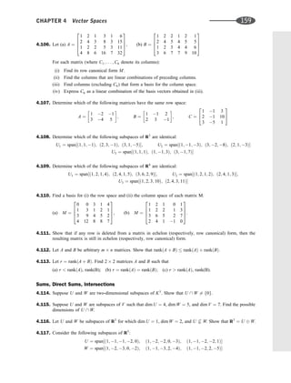
![(a) Find two homogeneous systems whose solution spaces are U and W, respectively.
(b) Find a basis and the dimension of U W.
4.118. Let U1, U2, U3 be the following subspaces of R3
:
U1 ¼ fða; b; cÞ : a ¼ cg; U2 ¼ fða; b; cÞ : a þ b þ c ¼ 0g; U3 ¼ fð0; 0; cÞg
Show that (a) R3
¼ U1 þ U2, (b) R3
¼ U2 þ U3, (c) R3
¼ U1 þ U3. When is the sum direct?
4.119. Suppose U, W1, W2 are subspaces of a vector space V. Show that
ðU W1Þ þ ðU W2Þ U ðW1 þ W2Þ
Find subspaces of R2
for which equality does not hold.
4.120. Suppose W1; W2; . . . ; Wr are subspaces of a vector space V. Show that
(a) spanðW1; W2; . . . ; WrÞ ¼ W1 þ W2 þ þ Wr.
(b) If Si spans Wi for i ¼ 1; . . . ; r, then S1 [ S2 [ [ Sr spans W1 þ W2 þ þ Wr.
4.121. Suppose V ¼ U W. Show that dim V ¼ dim U þ dim W.
4.122. Let S and T be arbitrary nonempty subsets (not necessarily subspaces) of a vector space V and let k be a
scalar. The sum S þ T and the scalar product kS are defined by
S þ T ¼ ðu þ v : u 2 S; v 2 Tg; kS ¼ fku : u 2 Sg
[We also write w þ S for fwg þ S.] Let
S ¼ fð1; 2Þ; ð2; 3Þg; T ¼ fð1; 4Þ; ð1; 5Þ; ð2; 5Þg; w ¼ ð1; 1Þ; k ¼ 3
Find: (a) S þ T, (b) w þ S, (c) kS, (d) kT, (e) kS þ kT, (f) kðS þ TÞ.
4.123. Show that the above operations of S þ T and kS satisfy
(a) Commutative law: S þ T ¼ T þ S.
(b) Associative law: ðS1 þ S2Þ þ S3 ¼ S1 þ ðS2 þ S3Þ.
(c) Distributive law: kðS þ TÞ ¼ kS þ kT.
(d) S þ f0g ¼ f0g þ S ¼ S and S þ V ¼ V þ S ¼ V.
4.124. Let V be the vector space of n-square matrices. Let U be the subspace of upper triangular matrices, and let
W be the subspace of lower triangular matrices. Find (a) U W, (b) U þ W.
4.125. Let V be the external direct sum of vector spaces U and W over a field K. (See Problem 4.76.) Let
^
U ¼ fðu; 0Þ : u 2 Ug and ^
W ¼ fð0; wÞ : w 2 Wg
Show that (a) ^
U and ^
W are subspaces of V, (b) V ¼ ^
U ^
W.
4.126. Suppose V ¼ U þ W. Let ^
V be the external direct sum of U and W. Show that V is isomorphic to ^
V under
the correspondence v ¼ u þ w $ ðu; wÞ.
4.127. Use induction to prove (a) Theorem 4.22, (b) Theorem 4.23.
Coordinates
4.128. The vectors u1 ¼ ð1; 2Þ and u2 ¼ ð4; 7Þ form a basis S of R2
. Find the coordinate vector ½v of v relative
to S where (a) v ¼ ð5; 3Þ, (b) v ¼ ða; bÞ.
4.129. The vectors u1 ¼ ð1; 2; 0Þ, u2 ¼ ð1; 3; 2Þ, u3 ¼ ð0; 1; 3Þ form a basis S of R3
. Find the coordinate vector ½v
of v relative to S where (a) v ¼ ð2; 7; 4Þ, (b) v ¼ ða; b; cÞ.
160 CHAPTER 4 Vector Spaces](https://image.slidesharecdn.com/linearalgebra4thedition-231030053714-df1faee2/85/Linear_Algebra-_4th_Edition-pdf-167-320.jpg)
![4.130. S ¼ ft3
þ t2
; t2
þ t; t þ 1; 1g is a basis of P3ðtÞ. Find the coordinate vector ½v of v relative to S
where (a) v ¼ 2t3
þ t2
4t þ 2, (b) v ¼ at3
þ bt2
þ ct þ d.
4.131. Let V ¼ M2;2. Find the coordinate vector [A] of A relative to S where
S ¼
1 1
1 1
;
1 1
1 0
;
1 1
0 0
;
1 0
0 0
and ðaÞ A ¼
3 5
6 7
; ðbÞ A ¼
a b
c d
4.132. Find the dimension and a basis of the subspace W of P3ðtÞ spanned by
u ¼ t3
þ 2t2
3t þ 4; v ¼ 2t3
þ 5t2
4t þ 7; w ¼ t3
þ 4t2
þ t þ 2
4.133. Find the dimension and a basis of the subspace W of M ¼ M2;3 spanned by
A ¼
1 2 1
3 1 2
; B ¼
2 4 3
7 5 6
; C ¼
1 2 3
5 7 6
Miscellaneous Problems
4.134. Answer true or false. If false, prove it with a counterexample.
(a) If u1, u2, u3 span V, then dim V ¼ 3.
(b) If A is a 4 8 matrix, then any six columns are linearly dependent.
(c) If u1, u2, u3 are linearly independent, then u1, u2, u3, w are linearly dependent.
(d) If u1, u2, u3, u4 are linearly independent, then dim V 4.
(e) If u1, u2, u3 span V, then w, u1, u2, u3 span V.
(f) If u1, u2, u3, u4 are linearly independent, then u1, u2, u3 are linearly independent.
4.135. Answer true or false. If false, prove it with a counterexample.
(a) If any column is deleted from a matrix in echelon form, then the resulting matrix is still in echelon
form.
(b) If any column is deleted from a matrix in row canonical form, then the resulting matrix is still in row
canonical form.
(c) If any column without a pivot is deleted from a matrix in row canonical form, then the resulting matrix
is in row canonical form.
4.136. Determine the dimension of the vector space W of the following n-square matrices:
(a) symmetric matrices, (b) antisymmetric matrices,
(d) diagonal matrices, (c) scalar matrices.
4.137. Let t1; t2; . . . ; tn be symbols, and let K be any field. Let V be the following set of expressions where ai 2 K:
a1t1 þ a2t2 þ þ antn
Define addition in V and scalar multiplication on V by
ða1t1 þ þ antnÞ þ ðb1t1 þ þ bntnÞ ¼ ða1 þ b1Þt1 þ þ ðanbnmÞtn
kða1t1 þ a2t2 þ þ antnÞ ¼ ka1t1 þ ka2t2 þ þ kantn
Show that V is a vector space over K with the above operations. Also, show that ft1; . . . ; tng is a basis of V,
where
tj ¼ 0t1 þ þ 0tj1 þ 1tj þ 0tjþ1 þ þ 0tn
CHAPTER 4 Vector Spaces 161](https://image.slidesharecdn.com/linearalgebra4thedition-231030053714-df1faee2/85/Linear_Algebra-_4th_Edition-pdf-168-320.jpg)
![ANSWERS TO SUPPLEMENTARY PROBLEMS
[Some answers, such as bases, need not be unique.]
4.71. (a) E1 ¼ 26u 22v; (b) The sum 7v þ 8 is not defined, so E2 is not defined;
(c) E3 ¼ 23u þ 5v; (d) Division by v is not defined, so E4 is not defined.
4.77. (a) Yes; (b) No; e.g., ð1; 2; 3Þ 2 W but 2ð1; 2; 3Þ 62 W;
(c) No; e.g., ð1; 0; 0Þ; ð0; 1; 0Þ 2 W, but not their sum; (d) Yes;
(e) No; e.g., ð1; 1; 1Þ 2 W, but 2ð1; 1; 1Þ 62 W; (f) Yes
4.79. The zero vector 0 is not a solution.
4.83. (a) w ¼ 3u1 u2, (b) Impossible, (c) k ¼ 11
5 , (d) 7a 5b þ c ¼ 0
4.84. Using f ¼ xp1 þ yp2 þ zp3, we get x ¼ a, y ¼ 2a þ b, z ¼ a þ b þ c
4.85. v ¼ ð2; 1; 0Þ
4.89. (a) Dependent, (b) Independent
4.90. (a) Independent, (b) Dependent
4.97. (a) u1, u2, u4; (b) u1, u2, u3; (c) u1, u2, u4; (d) u1, u2, u3
4.98. (a) dim U ¼ 3, (b) dim W ¼ 2, (c) dimðU WÞ ¼ 1
4.99. (a) Basis: fð2; 1; 0; 0; 0Þ; ð4; 0; 1; 1; 0Þ; ð3; 0; 1; 0; 1Þg; dim W ¼ 3;
(b) Basis: fð2; 1; 0; 0; 0Þ; ð1; 0; 1; 0; 0Þg; dim W ¼ 2
4.100. (a) 5x þ y z s ¼ 0; x þ y z t ¼ 0;
(b) 3x y z ¼ 0; 2x 3y þ s ¼ 0; x 2y þ t ¼ 0
4.101. (a) Yes, (b) No, because dim PnðtÞ ¼ n þ 1, but the set contains only n elements.
4.102. (a) dim W ¼ 2, (b) dim W ¼ 3
4.103. dim W ¼ 2
4.104. (a) 3, (b) 2, (c) 3
4.105. (a) n1 ¼ 4; n2 ¼ 5; n3 ¼ n4 ¼ n5 ¼ 0; (b) n1 ¼ 4; n2 ¼ 6; n3 ¼ 3; n4 ¼ n5 ¼ 0
4.106. (a) (i) M ¼ ½1; 2; 0; 1; 0; 3; 0; 0; 1; 2; 0; 1; 0; 0; 0; 0; 1; 2; 0;
(ii) C2, C4, C6; (iii) C1, C3, C5; (iv) C6 ¼ 3C1 þ C3 þ 2C5.
(b) (i) M ¼ ½1; 2; 0; 0; 3; 1; 0; 0; 1; 0; 1; 1; 0; 0; 0; 1; 1; 2; 0;
(ii) C2, C5, C6; (iii) C1, C3, C4; (iv) C6 ¼ C1 C3 þ 2C4
4.107. A and C are row equivalent to
1 0 7
0 1 4
, but not B
4.108. U1 and U2 are row equivalent to
1 0 2
0 1 1
, but not U3
4.109. U1 and U3 are row equivalent to
1 2 0 1
0 0 1 3
; but not U2
4.110. (a) (i) ð1; 3; 1; 2; 1Þ, ð0; 0; 1; 1; 1Þ, ð0; 0; 0; 4; 7Þ; (ii) C1, C3, C4;
(b) (i) ð1; 2; 1; 0; 1Þ, ð0; 0; 1; 1; 2Þ; (ii) C1, C3
162 CHAPTER 4 Vector Spaces](https://image.slidesharecdn.com/linearalgebra4thedition-231030053714-df1faee2/85/Linear_Algebra-_4th_Edition-pdf-169-320.jpg)
![4.113. (a) A ¼
1 1
0 0
; B ¼
1 1
0 0
; (b) A ¼
1 0
0 0
; B ¼
0 2
0 0
;
(c) A ¼
1 0
0 0
; B ¼
0 0
0 1
4.115. dimðU WÞ ¼ 2, 3, or 4
4.117. (a) (i)
3x þ 4y z t ¼ 0
4x þ 2y þ s ¼ 0
(ii)
4x þ 2y s ¼ 0
9x þ 2y þ z þ t ¼ 0
;
(b) Basis: fð1; 2; 5; 0; 0Þ; ð0; 0; 1; 0; 1Þg; dimðU WÞ ¼ 2
4.118. The sum is direct in (b) and (c).
4.119. In R2
, let U, V, W be, respectively, the line y ¼ x, the x-axis, the y-axis.
4.122. (a) fð2; 6Þ; ð2; 7Þ; ð3; 7Þ; ð3; 8Þ; ð4; 8Þg; (b) fð2; 3Þ; ð3; 4Þg;
(c) fð3; 6Þ; ð6; 9Þg; (d) fð3; 12Þ; ð3; 15Þ; ð6; 15Þg;
(e and f) fð6; 18Þ; ð6; 21Þ; ð9; 21Þ; ð9; 24Þ; ð12; 24Þg
4.124. (a) Diagonal matrices, (b) V
4.128. (a) [41; 11], (b) [7a 4b; 2a þ b]
4.129. (a) [11; 13; 10], (b) [c 3b þ 7a; c þ 3b 6a; c 2b þ 4a]
4.130. (a) [2; 1; 2; 2], (b) [a; b c; c b þ a; d c þ b a]
4.131. (a) [7; 1; 13; 10], (b) [d; c d; b þ c 2d; a b 2c þ 2d]
4.132. dim W ¼ 2; basis: ft3
þ 2t2
3t þ 4; t2
þ 2t 1g
4.133. dim W ¼ 2; basis: f½1; 2; 1; 3; 1; 2; ½0; 0; 1; 1; 3; 2g
4.134. (a) False; (1, 1), (1, 2), (2, 1) span R2
; (b) True;
(c) False; (1, 0, 0, 0), (0, 1, 0, 0), (0, 0, 1, 0), w ¼ ð0; 0; 0; 1Þ;
(d) True; (e) True; (f) True
4.135. (a) True; (b) False; e.g. delete C2 from
1 0 3
0 1 2
; (c) True
4.136. (a) 1
2 nðn þ 1Þ, (b) 1
2 nðn 1Þ, (c) n, (d) 1
CHAPTER 4 Vector Spaces 163](https://image.slidesharecdn.com/linearalgebra4thedition-231030053714-df1faee2/85/Linear_Algebra-_4th_Edition-pdf-170-320.jpg)
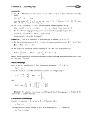
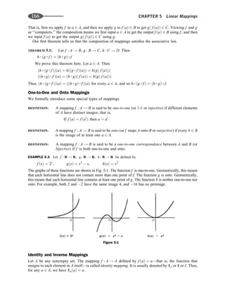
![Now let f : A ! B. We call g : B ! A the inverse of f, written f 1
, if
f g ¼ 1B and g f ¼ 1A
We emphasize that f has an inverse if and only if f is a one-to-one correspondence between A and B; that
is, f is one-to-one and onto (Problem 5.7). Also, if b 2 B, then f 1
ðbÞ ¼ a, where a is the unique element
of A for which f ðaÞ ¼ b
5.3 Linear Mappings (Linear Transformations)
We begin with a definition.
DEFINITION: Let V and U be vector spaces over the same field K. A mapping F : V ! U is called a
linear mapping or linear transformation if it satisfies the following two conditions:
(1) For any vectors v; w 2 V, Fðv þ wÞ ¼ FðvÞ þ FðwÞ.
(2) For any scalar k and vector v 2 V, FðkvÞ ¼ kFðvÞ.
Namely, F : V ! U is linear if it ‘‘preserves’’ the two basic operations of a vector space, that of
vector addition and that of scalar multiplication.
Substituting k ¼ 0 into condition (2), we obtain Fð0Þ ¼ 0. Thus, every linear mapping takes the zero
vector into the zero vector.
Now for any scalars a; b 2 K and any vector v; w 2 V, we obtain
Fðav þ bwÞ ¼ FðavÞ þ FðbwÞ ¼ aFðvÞ þ bFðwÞ
More generally, for any scalars ai 2 K and any vectors vi 2 V, we obtain the following basic property of
linear mappings:
Fða1v1 þ a2v2 þ þ amvmÞ ¼ a1Fðv1Þ þ a2Fðv2Þ þ þ amFðvmÞ
Remark 1: A linear mapping F : V ! U is completely characterized by the condition
Fðav þ bwÞ ¼ aFðvÞ þ bFðwÞ ð*Þ
and so this condition is sometimes used as its defintion.
Remark 2: The term linear transformation rather than linear mapping is frequently used for linear
mappings of the form F : Rn
! Rm
.
EXAMPLE 5.4
(a) Let F : R3
! R3
be the ‘‘projection’’ mapping into the xy-plane; that is, F is the mapping defined by
Fðx; y; zÞ ¼ ðx; y; 0Þ. We show that F is linear. Let v ¼ ða; b; cÞ and w ¼ ða0
; b0
; c0
Þ. Then
Fðv þ wÞ ¼ Fða þ a0
; b þ b0
; c þ c0
Þ ¼ ða þ a0
; b þ b0
; 0Þ
¼ ða; b; 0Þ þ ða0
; b0
; 0Þ ¼ FðvÞ þ FðwÞ
and, for any scalar k,
FðkvÞ ¼ Fðka; kb; kcÞ ¼ ðka; kb; 0Þ ¼ kða; b; 0Þ ¼ kFðvÞ
Thus, F is linear.
(b) Let G : R2
! R2
be the ‘‘translation’’ mapping defined by Gðx; yÞ ¼ ðx þ 1; y þ 2Þ. [That is, G adds the vector
(1, 2) to any vector v ¼ ðx; yÞ in R2
.] Note that
Gð0Þ ¼ Gð0; 0Þ ¼ ð1; 2Þ 6¼ 0
Thus, the zero vector is not mapped into the zero vector. Hence, G is not linear.
CHAPTER 5 Linear Mappings 167](https://image.slidesharecdn.com/linearalgebra4thedition-231030053714-df1faee2/85/Linear_Algebra-_4th_Edition-pdf-174-320.jpg)
![Vector Space Isomorphism
The notion of two vector spaces being isomorphic was defined in Chapter 4 when we investigated the
coordinates of a vector relative to a basis. We now redefine this concept.
DEFINITION: Two vector spaces V and U over K are isomorphic, written V ffi U, if there exists a
bijective (one-to-one and onto) linear mapping F : V ! U. The mapping F is then
called an isomorphism between V and U.
Consider any vector space V of dimension n and let S be any basis of V. Then the mapping
v 7! ½vS
which maps each vector v 2 V into its coordinate vector ½vS, is an isomorphism between V and Kn
.
5.4 Kernel and Image of a Linear Mapping
We begin by defining two concepts.
DEFINITION: Let F : V ! U be a linear mapping. The kernel of F, written Ker F, is the set of
elements in V that map into the zero vector 0 in U; that is,
Ker F ¼ fv 2 V : FðvÞ ¼ 0g
The image (or range) of F, written Im F, is the set of image points in U; that is,
Im F ¼ fu 2 U : there exists v 2 V for which FðvÞ ¼ ug
The following theorem is easily proved (Problem 5.22).
THEOREM 5.3: Let F : V ! U be a linear mapping. Then the kernel of F is a subspace of V and the
image of F is a subspace of U.
Now suppose that v1; v2; . . . ; vm span a vector space V and that F : V ! U is linear. We show that
Fðv1Þ; Fðv2Þ; . . . ; FðvmÞ span Im F. Let u 2 Im F. Then there exists v 2 V such that FðvÞ ¼ u. Because
the vi’s span V and v 2 V, there exist scalars a1; a2; . . . ; am for which
v ¼ a1v1 þ a2v2 þ þ amvm
Therefore,
u ¼ FðvÞ ¼ Fða1v1 þ a2v2 þ þ amvmÞ ¼ a1Fðv1Þ þ a2Fðv2Þ þ þ amFðvmÞ
Thus, the vectors Fðv1Þ; Fðv2Þ; . . . ; FðvmÞ span Im F.
We formally state the above result.
PROPOSITION 5.4: Suppose v1; v2; . . . ; vm span a vector space V, and suppose F : V ! U is linear.
Then Fðv1Þ; Fðv2Þ; . . . ; FðvmÞ span Im F.
EXAMPLE 5.7
(a) Let F : R3
! R3
be the projection of a vector v into the xy-plane [as pictured in Fig. 5-2(a)]; that is,
Fðx; y; zÞ ¼ ðx; y; 0Þ
Clearly the image of F is the entire xy-plane—that is, points of the form (x; y; 0). Moreover, the kernel of F is
the z-axis—that is, points of the form (0; 0; c). That is,
Im F ¼ fða; b; cÞ : c ¼ 0g ¼ xy-plane and Ker F ¼ fða; b; cÞ : a ¼ 0; b ¼ 0g ¼ z-axis
(b) Let G : R3
! R3
be the linear mapping that rotates a vector v about the z-axis through an angle y [as pictured in
Fig. 5-2(b)]; that is,
Gðx; y; zÞ ¼ ðx cos y y sin y; x sin y þ y cos y; zÞ
CHAPTER 5 Linear Mappings 169](https://image.slidesharecdn.com/linearalgebra4thedition-231030053714-df1faee2/85/Linear_Algebra-_4th_Edition-pdf-176-320.jpg)
![Observe that the distance of a vector v from the origin O does not change under the rotation, and so only the zero
vector 0 is mapped into the zero vector 0. Thus, Ker G ¼ f0g. On the other hand, every vector u in R3
is the image
of a vector v in R3
that can be obtained by rotating u back by an angle of y. Thus, Im G ¼ R3
, the entire space.
EXAMPLE 5.8 Consider the vector space V ¼ PðtÞ of polynomials over the real field R, and let H : V ! V be the
third-derivative operator; that is, H½ f ðtÞ ¼ d3
f =dt3
. [Sometimes the notation D3
is used for H, where D is the
derivative operator.] We claim that
Ker H ¼ fpolynomials of degree 2g ¼ P2ðtÞ and Im H ¼ V
The first comes from the fact that Hðat2
þ bt þ cÞ ¼ 0 but Hðtn
Þ 6¼ 0 for n 3. The second comes from that fact
that every polynomial gðtÞ in V is the third derivative of some polynomial f ðtÞ (which can be obtained by taking the
antiderivative of gðtÞ three times).
Kernel and Image of Matrix Mappings
Consider, say, a 3 4 matrix A and the usual basis fe1; e2; e3; e4g of K4
(written as columns):
A ¼
a1 a2 a3 a4
b1 b2 b3 b4
c1 c2 c3 c4
2
4
3
5; e1 ¼
1
0
0
0
2
6
6
4
3
7
7
5; e2 ¼
1
0
0
0
2
6
6
4
3
7
7
5; e3 ¼
1
0
0
0
2
6
6
4
3
7
7
5; e4 ¼
1
0
0
0
2
6
6
4
3
7
7
5
Recall that A may be viewed as a linear mapping A : K4
! K3
, where the vectors in K4
and K3
are
viewed as column vectors. Now the usual basis vectors span K4
, so their images Ae1, Ae2, Ae3, Ae4 span
the image of A. But the vectors Ae1, Ae2, Ae3, Ae4 are precisely the columns of A:
Ae1 ¼ ½a1; b1; c1T
; Ae2 ¼ ½a2; b2; c2T
; Ae3 ¼ ½a3; b3; c3T
; Ae4 ¼ ½a4; b4; c4T
Thus, the image of A is precisely the column space of A.
On the other hand, the kernel of A consists of all vectors v for which Av ¼ 0. This means that the
kernel of A is the solution space of the homogeneous system AX ¼ 0, called the null space of A.
We state the above results formally.
PROPOSITION 5.5: Let A be any m n matrix over a field K viewed as a linear map A : Kn
! Km
. Then
Ker A ¼ nullspðAÞ and Im A ¼ colspðAÞ
Here colsp(A) denotes the column space of A, and nullsp(A) denotes the null space of A.
Figure 5-2
170 CHAPTER 5 Linear Mappings](https://image.slidesharecdn.com/linearalgebra4thedition-231030053714-df1faee2/85/Linear_Algebra-_4th_Edition-pdf-177-320.jpg)
![THEOREM 5.12: Let V, U, W be vector spaces over K. Suppose the following mappings are linear:
F : V ! U; F0
: V ! U and G : U ! W; G0
: U ! W
Then, for any scalar k 2 K:
(i) G ðF þ F0
Þ ¼ G F þ G F0
.
(ii) ðG þ G0
Þ F ¼ G F þ G0 F.
(iii) kðG FÞ ¼ ðkGÞ F ¼ G ðkFÞ.
5.7 Algebra AðVÞ of Linear Operators
Let V be a vector space over a field K. This section considers the special case of linear mappings from the
vector space V into itself—that is, linear mappings of the form F : V ! V. They are also called linear
operators or linear transformations on V. We will write AðVÞ, instead of HomðV; VÞ, for the space of all
such mappings.
Now AðVÞ is a vector space over K (Theorem 5.8), and, if dim V ¼ n, then dim AðVÞ ¼ n2
. Moreover,
for any mappings F; G 2 AðVÞ, the composition G F exists and also belongs to AðVÞ. Thus, we have a
‘‘multiplication’’ defined in AðVÞ. [We sometimes write FG instead of G F in the space AðVÞ.]
Remark: An algebra A over a field K is a vector space over K in which an operation of
multiplication is defined satisfying, for every F; G; H 2 A and every k 2 K:
(i) FðG þ HÞ ¼ FG þ FH,
(ii) ðG þ HÞF ¼ GF þ HF,
(iii) kðGFÞ ¼ ðkGÞF ¼ GðkFÞ.
The algebra is said to be associative if, in addition, ðFGÞH ¼ FðGHÞ.
The above definition of an algebra and previous theorems give us the following result.
THEOREM 5.13: Let V be a vector space over K. Then AðVÞ is an associative algebra over K with
respect to composition of mappings. If dim V ¼ n, then dim AðVÞ ¼ n2
.
This is why AðVÞ is called the algebra of linear operators on V.
Polynomials and Linear Operators
Observe that the identity mapping I : V ! V belongs to AðVÞ. Also, for any linear operator F in AðVÞ,
we have FI ¼ IF ¼ F. We can also form ‘‘powers’’ of F. Namely, we define
F0
¼ I; F2
¼ F F; F3
¼ F2 F ¼ F F F; F4
¼ F3 F; . . .
Furthermore, for any polynomial pðtÞ over K, say,
pðtÞ ¼ a0 þ a1t þ a2t2
þ þ ast2
we can form the linear operator pðFÞ defined by
pðFÞ ¼ a0I þ a1F þ a2F2
þ þ asFs
(For any scalar k, the operator kI is sometimes denoted simply by k.) In particular, we say F is a zero of
the polynomial pðtÞ if pðFÞ ¼ 0.
EXAMPLE 5.11 Let F : K3
! K3
be defined by Fðx; y; zÞ ¼ ð0; x; yÞ. For any ða; b; cÞ 2 K3
,
ðF þ IÞða; b; cÞ ¼ ð0; a; bÞ þ ða; b; cÞ ¼ ða; a þ b; b þ cÞ
F3
ða; b; cÞ ¼ F2
ð0; a; bÞ ¼ Fð0; 0; aÞ ¼ ð0; 0; 0Þ
Thus, F3
¼ 0, the zero mapping in AðVÞ. This means F is a zero of the polynomial pðtÞ ¼ t3
.
174 CHAPTER 5 Linear Mappings](https://image.slidesharecdn.com/linearalgebra4thedition-231030053714-df1faee2/85/Linear_Algebra-_4th_Edition-pdf-181-320.jpg)
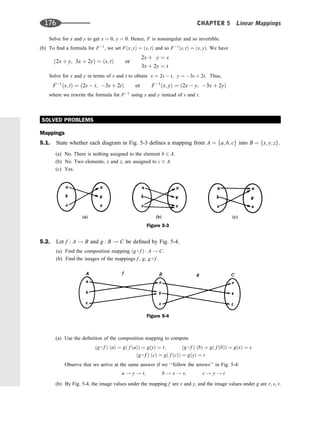
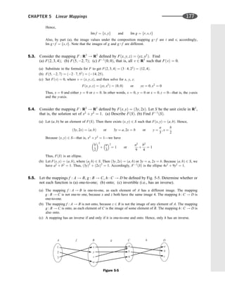
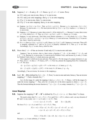
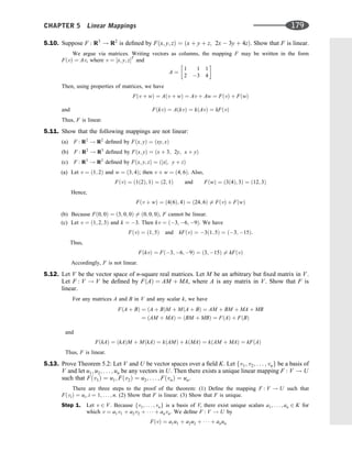
![(Because the ai are unique, the mapping F is well defined.) Now, for i ¼ 1; . . . ; n,
vi ¼ 0v1 þ þ 1vi þ þ 0vn
Hence,
FðviÞ ¼ 0u1 þ þ 1ui þ þ 0un ¼ ui
Thus, the first step of the proof is complete.
Step 2. Suppose v ¼ a1v1 þ a2v2 þ þ anvn and w ¼ b1v1 þ b2v2 þ þ bnvn. Then
v þ w ¼ ða1 þ b1Þv1 þ ða2 þ b2Þv2 þ þ ðan þ bnÞvn
and, for any k 2 K, kv ¼ ka1v1 þ ka2v2 þ þ kanvn. By definition of the mapping F,
FðvÞ ¼ a1u1 þ a2u2 þ þ anvn and FðwÞ ¼ b1u1 þ b2u2 þ þ bnun
Hence,
Fðv þ wÞ ¼ ða1 þ b1Þu1 þ ða2 þ b2Þu2 þ þ ðan þ bnÞun
¼ ða1u1 þ a2u2 þ þ anunÞ þ ðb1u1 þ b2u2 þ þ bnunÞ
¼ FðvÞ þ FðwÞ
and
FðkvÞ ¼ kða1u1 þ a2u2 þ þ anunÞ ¼ kFðvÞ
Thus, F is linear.
Step 3. Suppose G : V ! U is linear and Gðv1Þ ¼ ui; i ¼ 1; . . . ; n. Let
v ¼ a1v1 þ a2v2 þ þ anvn
Then
GðvÞ ¼ Gða1v1 þ a2v2 þ þ anvnÞ ¼ a1Gðv1Þ þ a2Gðv2Þ þ þ anGðvnÞ
¼ a1u1 þ a2u2 þ þ anun ¼ FðvÞ
Because GðvÞ ¼ FðvÞ for every v 2 V; G ¼ F. Thus, F is unique and the theorem is proved.
5.14. Let F : R2
! R2
be the linear mapping for which Fð1; 2Þ ¼ ð2; 3Þ and Fð0; 1Þ ¼ ð1; 4Þ. [Note that
fð1; 2Þ; ð0; 1Þg is a basis of R2
, so such a linear map F exists and is unique by Theorem 5.2.] Find
a formula for F; that is, find Fða; bÞ.
Write ða; bÞ as a linear combination of (1, 2) and (0, 1) using unknowns x and y,
ða; bÞ ¼ xð1; 2Þ þ yð0; 1Þ ¼ ðx; 2x þ yÞ; so a ¼ x; b ¼ 2x þ y
Solve for x and y in terms of a and b to get x ¼ a, y ¼ 2a þ b. Then
Fða; bÞ ¼ xFð1; 2Þ þ yFð0; 1Þ ¼ að2; 3Þ þ ð2a þ bÞð1; 4Þ ¼ ðb; 5a þ 4bÞ
5.15. Suppose a linear mapping F : V ! U is one-to-one and onto. Show that the inverse mapping
F1
: U ! V is also linear.
Suppose u; u0
2 U. Because F is one-to-one and onto, there exist unique vectors v; v0
2 V for which
FðvÞ ¼ u and Fðv0
Þ ¼ u0
. Because F is linear, we also have
Fðv þ v0
Þ ¼ FðvÞ þ Fðv0
Þ ¼ u þ u0
and FðkvÞ ¼ kFðvÞ ¼ ku
By definition of the inverse mapping,
F1
ðuÞ ¼ v; F1
ðu0
Þ ¼ v0
; F1
ðu þ u0
Þ ¼ v þ v0
; F1
ðkuÞ ¼ kv:
Then
F1
ðu þ u0
Þ ¼ v þ v0
¼ F1
ðuÞ þ F1
ðu0
Þ and F1
ðkuÞ ¼ kv ¼ kF1
ðuÞ
Thus, F1
is linear.
180 CHAPTER 5 Linear Mappings](https://image.slidesharecdn.com/linearalgebra4thedition-231030053714-df1faee2/85/Linear_Algebra-_4th_Edition-pdf-187-320.jpg)
![Kernel and Image of Linear Mappings
5.16. Let F : R4
! R3
be the linear mapping defined by
Fðx; y; z; tÞ ¼ ðx y þ z þ t; x þ 2z t; x þ y þ 3z 3tÞ
Find a basis and the dimension of (a) the image of F; (b) the kernel of F.
(a) Find the images of the usual basis of R4
:
Fð1; 0; 0; 0Þ ¼ ð1; 1; 1Þ; Fð0; 0; 1; 0Þ ¼ ð1; 2; 3Þ
Fð0; 1; 0; 0Þ ¼ ð1; 0; 1Þ; Fð0; 0; 0; 1Þ ¼ ð1; 1; 3Þ
By Proposition 5.4, the image vectors span Im F. Hence, form the matrix whose rows are these image
vectors, and row reduce to echelon form:
1 1 1
1 0 1
1 2 3
1 1 3
2
6
6
6
4
3
7
7
7
5
1 1 1
0 1 2
0 1 2
0 2 4
2
6
6
6
4
3
7
7
7
5
1 1 1
0 1 2
0 0 0
0 0 0
2
6
6
6
4
3
7
7
7
5
Thus, (1, 1, 1) and (0, 1, 2) form a basis for Im F; hence, dimðIm FÞ ¼ 2.
(b) Set FðvÞ ¼ 0, where v ¼ ðx; y; z; tÞ; that is, set
Fðx; y; z; tÞ ¼ ðx y þ z þ t; x þ 2z t; x þ y þ 3z 3tÞ ¼ ð0; 0; 0Þ
Set corresponding entries equal to each other to form the following homogeneous system whose solution
space is Ker F:
x y þ z þ t ¼ 0
x þ 2z t ¼ 0
x þ y þ 3z 3t ¼ 0
or
x y þ z þ t ¼ 0
y þ z 2t ¼ 0
2y þ 2z 4t ¼ 0
or
x y þ z þ t ¼ 0
y þ z 2t ¼ 0
The free variables are z and t. Hence, dimðKer FÞ ¼ 2.
(i) Set z ¼ 1, t ¼ 0 to obtain the solution (2; 1; 1; 0).
(ii) Set z ¼ 0, t ¼ 1 to obtain the solution (1, 2, 0, 1).
Thus, (2; 1; 1; 0) and (1, 2, 0, 1) form a basis of Ker F.
[As expected, dimðIm FÞ þ dimðKer FÞ ¼ 2 þ 2 ¼ 4 ¼ dim R4
, the domain of F.]
5.17. Let G : R3
! R3
be the linear mapping defined by
Gðx; y; zÞ ¼ ðx þ 2y z; y þ z; x þ y 2zÞ
Find a basis and the dimension of (a) the image of G, (b) the kernel of G.
(a) Find the images of the usual basis of R3
:
Gð1; 0; 0Þ ¼ ð1; 0; 1Þ; Gð0; 1; 0Þ ¼ ð2; 1; 1Þ; Gð0; 0; 1Þ ¼ ð1; 1; 2Þ
By Proposition 5.4, the image vectors span Im G. Hence, form the matrix M whose rows are these image
vectors, and row reduce to echelon form:
M ¼
1 0 1
2 1 1
1 1 2
2
4
3
5
1 0 1
0 1 1
0 1 1
2
4
3
5
1 0 1
0 1 1
0 0 0
2
4
3
5
Thus, (1, 0, 1) and (0; 1; 1) form a basis for Im G; hence, dimðIm GÞ ¼ 2.
(b) Set GðvÞ ¼ 0, where v ¼ ðx; y; zÞ; that is,
Gðx; y; zÞ ¼ ðx þ 2y z; y þ z; x þ y 2zÞ ¼ ð0; 0; 0Þ
CHAPTER 5 Linear Mappings 181](https://image.slidesharecdn.com/linearalgebra4thedition-231030053714-df1faee2/85/Linear_Algebra-_4th_Edition-pdf-188-320.jpg)
![Set corresponding entries equal to each other to form the following homogeneous system whose solution
space is Ker G:
x þ 2y z ¼ 0
y þ z ¼ 0
x þ y 2z ¼ 0
or
x þ 2y z ¼ 0
y þ z ¼ 0
y z ¼ 0
or
x þ 2y z ¼ 0
y þ z ¼ 0
The only free variable is z; hence, dimðKer GÞ ¼ 1. Set z ¼ 1; then y ¼ 1 and x ¼ 3. Thus, (3; 1; 1)
forms a basis of Ker G. [As expected, dimðIm GÞ þ dimðKer GÞ ¼ 2 þ 1 ¼ 3 ¼ dim R3
, the domain
of G.]
5.18. Consider the matrix mapping A : R4
! R3
, where A ¼
1 2 3 1
1 3 5 2
3 8 13 3
2
4
3
5. Find a basis and the
dimension of (a) the image of A, (b) the kernel of A.
(a) The column space of A is equal to Im A. Now reduce AT
to echelon form:
AT
¼
1 1 3
2 3 8
3 5 13
1 2 3
2
6
6
4
3
7
7
5
1 1 3
0 1 2
0 2 4
0 3 6
2
6
6
4
3
7
7
5
1 1 3
0 1 2
0 0 0
0 0 0
2
6
6
4
3
7
7
5
Thus, fð1; 1; 3Þ; ð0; 1; 2Þg is a basis of Im A, and dimðIm AÞ ¼ 2.
(b) Here Ker A is the solution space of the homogeneous system AX ¼ 0, where X ¼ fx; y; z; tÞT
. Thus,
reduce the matrix A of coefficients to echelon form:
1 2 3 1
0 1 2 3
0 2 4 6
2
4
3
5
1 2 3 1
0 1 2 3
0 0 0 0
2
4
3
5 or
x þ 2y þ 3z þ t ¼ 0
y þ 2z 3t ¼ 0
The free variables are z and t. Thus, dimðKer AÞ ¼ 2.
(i) Set z ¼ 1, t ¼ 0 to get the solution (1; 2; 1; 0).
(ii) Set z ¼ 0, t ¼ 1 to get the solution (7; 3; 0; 1).
Thus, (1; 2; 1; 0) and (7; 3; 0; 1) form a basis for Ker A.
5.19. Find a linear map F : R3
! R4
whose image is spanned by (1; 2; 0; 4) and (2; 0; 1; 3).
Form a 4 3 matrix whose columns consist only of the given vectors, say
A ¼
1 2 2
2 0 0
0 1 1
4 3 3
2
6
6
4
3
7
7
5
Recall that A determines a linear map A : R3
! R4
whose image is spanned by the columns of A. Thus, A
satisfies the required condition.
5.20. Suppose f : V ! U is linear with kernel W, and that f ðvÞ ¼ u. Show that the ‘‘coset’’
v þ W ¼ fv þ w : w 2 Wg is the preimage of u; that is, f 1
ðuÞ ¼ v þ W.
We must prove that (i) f 1
ðuÞ v þ W and (ii) v þ W f 1
ðuÞ.
We first prove (i). Suppose v0
2 f 1
ðuÞ. Then f ðv0
Þ ¼ u, and so
f ðv0
vÞ ¼ f ðv0
Þ f ðvÞ ¼ u u ¼ 0
that is, v0
v 2 W. Thus, v0
¼ v þ ðv0
vÞ 2 v þ W, and hence f 1
ðuÞ v þ W.
182 CHAPTER 5 Linear Mappings](https://image.slidesharecdn.com/linearalgebra4thedition-231030053714-df1faee2/85/Linear_Algebra-_4th_Edition-pdf-189-320.jpg)
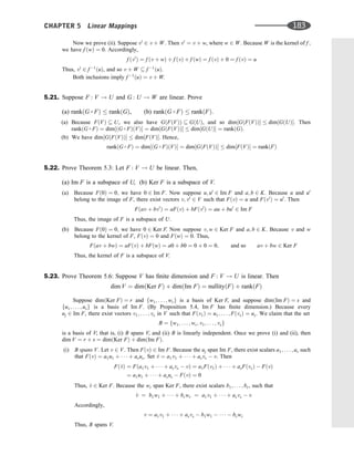
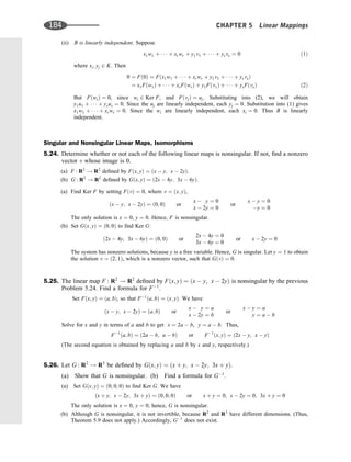
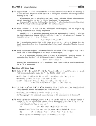
![5.33. Suppose F1; F2; . . . ; Fn are linear maps from V into U. Show that, for any scalars a1; a2; . . . ; an,
and for any v 2 V,
ða1F1 þ a2F2 þ þ anFnÞðvÞ ¼ a1F1ðvÞ þ a2F2ðvÞ þ þ anFnðvÞ
The mapping a1F1 is defined by ða1F1ÞðvÞ ¼ a1FðvÞ. Hence, the theorem holds for n ¼ 1. Accordingly,
by induction,
ða1F1 þ a2F2 þ þ anFnÞðvÞ ¼ ða1F1ÞðvÞ þ ða2F2 þ þ anFnÞðvÞ
¼ a1F1ðvÞ þ a2F2ðvÞ þ þ anFnðvÞ
5.34. Consider linear mappings F : R3
! R2
, G : R3
! R2
, H : R3
! R2
defined by
Fðx; y; zÞ ¼ ðx þ y þ z; x þ yÞ; Gðx; y; zÞ ¼ ð2x þ z; x þ yÞ; Hðx; y; zÞ ¼ ð2y; xÞ
Show that F, G, H are linearly independent [as elements of HomðR3
; R2
Þ].
Suppose, for scalars a; b; c 2 K,
aF þ bG þ cH ¼ 0 ð1Þ
(Here 0 is the zero mapping.) For e1 ¼ ð1; 0; 0Þ 2 R3
, we have 0ðe1Þ ¼ ð0; 0Þ and
ðaF þ bG þ cHÞðe1Þ ¼ aFð1; 0; 0Þ þ bGð1; 0; 0Þ þ cHð1; 0; 0Þ
¼ að1; 1Þ þ bð2; 1Þ þ cð0; 1Þ ¼ ða þ 2b; a þ b þ cÞ
Thus by (1), ða þ 2b; a þ b þ cÞ ¼ ð0; 0Þ and so
a þ 2b ¼ 0 and a þ b þ c ¼ 0 ð2Þ
Similarly for e2 ¼ ð0; 1; 0Þ 2 R3
, we have 0ðe2Þ ¼ ð0; 0Þ and
ðaF þ bG þ cHÞðe2Þ ¼ aFð0; 1; 0Þ þ bGð0; 1; 0Þ þ cHð0; 1; 0Þ
¼ að1; 1Þ þ bð0; 1Þ þ cð2; 0Þ ¼ ða þ 2c; a þ bÞ
Thus,
a þ 2c ¼ 0 and a þ b ¼ 0 ð3Þ
Using (2) and (3), we obtain
a ¼ 0; b ¼ 0; c ¼ 0 ð4Þ
Because (1) implies (4), the mappings F, G, H are linearly independent.
5.35. Let k be a nonzero scalar. Show that a linear map T is singular if and only if kT is singular. Hence,
T is singular if and only if T is singular.
Suppose T is singular. Then TðvÞ ¼ 0 for some vector v 6¼ 0. Hence,
ðkTÞðvÞ ¼ kTðvÞ ¼ k0 ¼ 0
and so kT is singular.
Now suppose kT is singular. Then ðkTÞðwÞ ¼ 0 for some vector w 6¼ 0. Hence,
TðkwÞ ¼ kTðwÞ ¼ ðkTÞðwÞ ¼ 0
But k 6¼ 0 and w 6¼ 0 implies kw 6¼ 0. Thus, T is also singular.
5.36. Find the dimension d of:
(a) HomðR3
; R4
Þ, (b) HomðR5
; R3
Þ, (c) HomðP3ðtÞ; R2
Þ, (d) HomðM2;3; R4
Þ.
Use dim½HomðV; UÞ ¼ mn, where dim V ¼ m and dim U ¼ n.
(a) d ¼ 3ð4Þ ¼ 12. (c) Because dim P3ðtÞ ¼ 4, d ¼ 4ð2Þ ¼ 8.
(b) d ¼ 5ð3Þ ¼ 15. (d) Because dim M2;3 ¼ 6, d ¼ 6ð4Þ ¼ 24.
186 CHAPTER 5 Linear Mappings](https://image.slidesharecdn.com/linearalgebra4thedition-231030053714-df1faee2/85/Linear_Algebra-_4th_Edition-pdf-193-320.jpg)
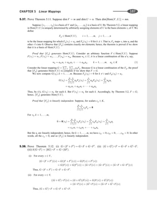
![(iii) For every v 2 V,
ðkðG FÞÞðvÞ ¼ kðG FÞðvÞ ¼ kðGðFðvÞÞÞ ¼ ðkGÞðFðvÞÞ ¼ ðkG FÞðvÞ
and
ðkðG FÞÞðvÞ ¼ kðG FÞðvÞ ¼ kðGðFðvÞÞÞ ¼ GðkFðvÞÞ ¼ GððkFÞðvÞÞ ¼ ðG kFÞðvÞ
Accordingly, kðG FÞ ¼ ðkGÞ F ¼ G ðkFÞ. (We emphasize that two mappings are shown to be equal
by showing that each of them assigns the same image to each point in the domain.)
Algebra of Linear Maps
5.39. Let F and G be the linear operators on R2
defined by Fðx; yÞ ¼ ðy; xÞ and Gðx; yÞ ¼ ð0; xÞ. Find
formulas defining the following operators:
(a) F þ G, (b) 2F 3G, (c) FG, (d) GF, (e) F2
, (f) G2
.
(a) ðF þ GÞðx; yÞ ¼ Fðx; yÞ þ Gðx; yÞ ¼ ðy; xÞ þ ð0; xÞ ¼ ðy; 2xÞ.
(b) ð2F 3GÞðx; yÞ ¼ 2Fðx; yÞ 3Gðx; yÞ ¼ 2ðy; xÞ 3ð0; xÞ ¼ ð2y; xÞ.
(c) ðFGÞðx; yÞ ¼ FðGðx; yÞÞ ¼ Fð0; xÞ ¼ ðx; 0Þ.
(d) ðGFÞðx; yÞ ¼ GðFðx; yÞÞ ¼ Gðy; xÞ ¼ ð0; yÞ.
(e) F2
ðx; yÞ ¼ FðFðx; yÞÞ ¼ Fðy; xÞ ¼ ðx; yÞ. (Note that F2
¼ I, the identity mapping.)
(f) G2
ðx; yÞ ¼ GðGðx; yÞÞ ¼ Gð0; xÞ ¼ ð0; 0Þ. (Note that G2
¼ 0, the zero mapping.)
5.40. Consider the linear operator T on R3
defined by Tðx; y; zÞ ¼ ð2x; 4x y; 2x þ 3y zÞ.
(a) Show that T is invertible. Find formulas for (b) T1
, (c) T2
, (d) T2
.
(a) Let W ¼ Ker T. We need only show that T is nonsingular (i.e., that W ¼ f0g). Set Tðx; y; zÞ ¼ ð0; 0; 0Þ,
which yields
Tðx; y; zÞ ¼ ð2x; 4x y; 2x þ 3y zÞ ¼ ð0; 0; 0Þ
Thus, W is the solution space of the homogeneous system
2x ¼ 0; 4x y ¼ 0; 2x þ 3y z ¼ 0
which has only the trivial solution (0, 0, 0). Thus, W ¼ f0g. Hence, T is nonsingular, and so T is
invertible.
(b) Set Tðx; y; zÞ ¼ ðr; s; tÞ [and so T1
ðr; s; tÞ ¼ ðx; y; zÞ]. We have
ð2x; 4x y; 2x þ 3y zÞ ¼ ðr; s; tÞ or 2x ¼ r; 4x y ¼ s; 2x þ 3y z ¼ t
Solve for x, y, z in terms of r, s, t to get x ¼ 1
2 r, y ¼ 2r s, z ¼ 7r 3s t. Thus,
T1
ðr; s; tÞ ¼ ð1
2 r; 2r s; 7r 3s tÞ or T1
ðx; y; zÞ ¼ ð1
2 x; 2x y; 7x 3y zÞ
(c) Apply T twice to get
T2
ðx; y; zÞ ¼ Tð2x; 4x y; 2x þ 3y zÞ
¼ ½4x; 4ð2xÞ ð4x yÞ; 2ð2xÞ þ 3ð4x yÞ ð2x þ 3y zÞ
¼ ð4x; 4x þ y; 14x 6y þ zÞ
(d) Apply T1
twice to get
T2
ðx; y; zÞ ¼ T2
ð1
2 x; 2x y; 7x 3y zÞ
¼ ½1
4 x; 2ð1
2 xÞ ð2x yÞ; 7ð1
2 xÞ 3ð2x yÞ ð7x 3y zÞ
¼ ð1
4 x; x þ y; 19
2 x þ 6y þ zÞ
188 CHAPTER 5 Linear Mappings](https://image.slidesharecdn.com/linearalgebra4thedition-231030053714-df1faee2/85/Linear_Algebra-_4th_Edition-pdf-195-320.jpg)
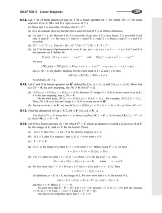
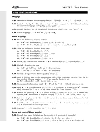
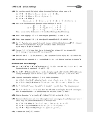
![5.90. Let F : V ! U be linear and let W be a subspace of V. The restriction of F to W is the map FjW : W ! U
defined by FjWðvÞ ¼ FðvÞ for every v in W. Prove the following:
(a) FjW is linear; (b) KerðFjWÞ ¼ ðKer FÞ W; (c) ImðFjWÞ ¼ FðWÞ.
5.91. A subset X of a vector space V is said to be convex if the line segment L between any two points (vectors)
P; Q 2 X is contained in X. (a) Show that the intersection of convex sets is convex; (b) suppose F : V ! U
is linear and X is convex. Show that FðXÞ is convex.
ANSWERS TO SUPPLEMENTARY PROBLEMS
5.45. ðaÞ 32
¼ 9; ðbÞ sr
5.46. (a) ð f gÞðxÞ ¼ 4x2
þ 1, (b) ðg f ÞðxÞ ¼ 2x2
þ 6x 1, (c) ðg gÞðxÞ ¼ 4x 9,
(d) ð f f ÞðxÞ ¼ x4
þ 6x3
þ 14x2
þ 15x þ 5
5.47. (a) f 1
ðxÞ ¼ 1
3 ðx þ 7Þ, (b) f 1
ðxÞ ¼
ffiffiffiffiffiffiffiffiffiffiffi
x 2
3
p
5.49. Fðx; y; zÞ ¼ Aðx; y; zÞT
, where (a) A ¼
1 2 3
4 5 6
, (b) A ¼
a b
c d
5.50. (a) u ¼ ð2; 2Þ, k ¼ 3; then FðkuÞ ¼ ð36; 36Þ but kFðuÞ ¼ ð12; 12Þ; (b) Fð0Þ 6¼ 0;
(c) u ¼ ð1; 2Þ, v ¼ ð3; 4Þ; then Fðu þ vÞ ¼ ð24; 6Þ but FðuÞ þ FðvÞ ¼ ð14; 6Þ;
(d) u ¼ ð1; 2; 3Þ, k ¼ 2; then FðkuÞ ¼ ð2; 10Þ but kFðuÞ ¼ ð2; 10Þ.
5.51. Fða; bÞ ¼ ða þ 2b; 3a þ bÞ
5.52. (a) A ¼
17 5
23 6
; (b) None. (2; 4) and (1; 2) are linearly dependent but not (1, 1) and (1, 3).
5.53. B ¼
1 0
3 0
[Hint: Send ð0; 1ÞT
into ð0; 0ÞT
.]
5.55. Fðx; yÞ ¼ ðx2
; y2
Þ
5.56. (a) 13x2
42xy þ 34y2
¼ 1, (b) 13x2
þ 42xy þ 34y2
¼ 1
5.57. (a) x2
8xy þ 26y2
þ 6xz 38yz þ 14z2
¼ 1, (b) x2
þ 2xy þ 3y2
þ 2xz 8yz þ 14z2
¼ 1
5.58. (a) x y þ 2z ¼ 4, (b) x þ 6z ¼ 4
5.61. (a) dimðKer FÞ ¼ 1, fð7; 2; 1Þg; dimðIm FÞ ¼ 2, fð1; 2; 1Þ; ð0; 1; 2Þg;
(b) dimðKer FÞ ¼ 2, fð2; 1; 0; 0Þ; ð1; 0; 1; 1Þg; dimðIm FÞ ¼ 2, fð1; 2; 1Þ; ð0; 1; 3Þg
5.62. (a) dimðKer GÞ ¼ 2, fð1; 0; 1Þ; ð1; 1; 0Þg; dimðIm GÞ ¼ 1, fð1; 2Þg;
(b) dimðKer GÞ ¼ 1, fð1; 1; 1Þg; Im G ¼ R2
, fð1; 0Þ; ð0; 1Þg;
(c) dimðKer GÞ ¼ 3, fð2; 1; 0; 0; 0Þ; ð1; 0; 1; 1; 0Þ; ð5; 0; 2; 0; 1Þg; dimðIm GÞ ¼ 2,
fð1; 1; 3Þ; ð0; 1; 2Þg
5.63. (a) dimðKer AÞ ¼ 2, fð4; 2; 5; 0Þ; ð1; 3; 0; 5Þg; dimðIm AÞ ¼ 2, fð1; 2; 1Þ; ð0; 1; 1Þg;
(b) dimðKer BÞ ¼ 1, fð1; 2
3 ; 1; 1Þg; Im B ¼ R3
5.64. Fðx; y; zÞ ¼ ðx þ 4y; 2x þ 5y; 3x þ 6yÞ
CHAPTER 5 Linear Mappings 193](https://image.slidesharecdn.com/linearalgebra4thedition-231030053714-df1faee2/85/Linear_Algebra-_4th_Edition-pdf-200-320.jpg)
![5.65. Fðx; y; z; tÞ ¼ ðx þ y z; 2x þ y t; 0Þ
5.66. (a) f1; t; t2
; . . . ; t6
g, (b) f1; t; t2
; t3
g
5.68. None, because dim R4
dim R3
:
5.69. Ker 0 ¼ V, Im 0 ¼ f0g
5.70. ðF þ GÞðx; y; zÞ ¼ ðy þ 2z; 2x y þ zÞ, ð3F 2GÞðx; y; zÞ ¼ ð3y 4z; x þ 2y þ 3zÞ
5.71. (a) ðH FÞðx; y; zÞ ¼ ðx þ z; 2yÞ, ðH GÞðx; y; zÞ ¼ ðx y; 4zÞ; (b) not defined;
(c) ðH ðF þ GÞÞðx; y; zÞ ¼ ðH F þ H GÞðx; y; zÞ ¼ ð2x y þ z; 2y þ 4zÞ
5.74. Fðx; yÞ ¼ ðx; y; yÞ; Gðx; y; zÞ ¼ ðx; yÞ
5.75. (a) 16, (b) 15, (c) 24
5.76. (a) v ¼ ð2; 3; 1Þ; (b) G1
ðat2
þ bt þ cÞ ¼ ðb 2c; a b þ 2c; a þ b cÞ;
(c) H is nonsingular, but not invertible, because dim P2ðtÞ dim R2
.
5.77. dim U ¼ 1; that is, U ¼ K.
5.78. (a) ðF þ GÞðx; yÞ ¼ ðx; xÞ; (b) ð5F 3GÞðx; yÞ ¼ ð5x þ 8y; 3xÞ; (c) ðFGÞðx; yÞ ¼ ðx y; 0Þ;
(d) ðGFÞðx; yÞ ¼ ð0; x þ yÞ; (e) F2
ðx; yÞ ¼ ðx þ y; 0Þ (note that F2
¼ F); ( f ) G2
ðx; yÞ ¼ ðx; yÞ.
[Note that G2
þ I ¼ 0; hence, G is a zero of f ðtÞ ¼ t2
þ 1.]
5.79. (a) T1
ðx; yÞ ¼ ð3x þ 2y; 2x yÞ, (b) T1
ðx; yÞ ¼ ð4x þ 3y; 3x þ 2yÞ
5.80. (a) T1
ðx; y; zÞ ¼ ðx þ 3y þ 14z; y 4z; zÞ, (b) T1
ðx; y; zÞ ¼ ðy þ z; y; x y zÞ
5.81. (a) 49, (b) 36, (c) 144
5.82. Squares: 9, 25, 36, 64, 100
5.83. (a) Tðx; yÞ ¼ ð6x þ 14y; 21x þ 27yÞ; (b) Tðx; yÞ ¼ ð0; 0Þ—that is, f ðTÞ ¼ 0
194 CHAPTER 5 Linear Mappings](https://image.slidesharecdn.com/linearalgebra4thedition-231030053714-df1faee2/85/Linear_Algebra-_4th_Edition-pdf-201-320.jpg)
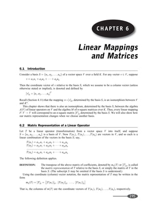
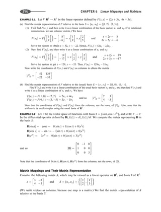
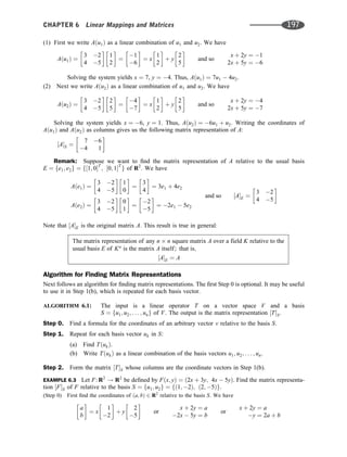
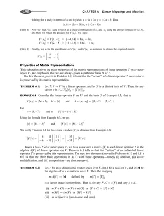
![THEOREM 6.3: For any linear operators F; G 2 AðVÞ,
mðG FÞ ¼ mðGÞmðFÞ or ½G F ¼ ½G½F
(Here G F denotes the composition of the maps G and F.)
6.3 Change of Basis
Let V be an n-dimensional vector space over a field K. We have shown that once we have selected a basis
S of V, every vector v 2 V can be represented by means of an n-tuple ½vS in Kn
, and every linear operator
T in AðVÞ can be represented by an n n matrix over K. We ask the following natural question:
How do our representations change if we select another basis?
In order to answer this question, we first need a definition.
DEFINITION: Let S ¼ fu1; u2; . . . ; ung be a basis of a vector space V; and let S0
¼ fv1; v2; . . . ; vng
be another basis. (For reference, we will call S the ‘‘old’’ basis and S0
the ‘‘new’’
basis.) Because S is a basis, each vector in the ‘‘new’’ basis S0
can be written uniquely
as a linear combination of the vectors in S; say,
v1 ¼ a11u1 þ a12u2 þ þ a1nun
v2 ¼ a21u1 þ a22u2 þ þ a2nun
:::::::::::::::::::::::::::::::::::::::::::::::::
vn ¼ an1u1 þ an2u2 þ þ annun
Let P be the transpose of the above matrix of coefficients; that is, let P ¼ ½pij, where
pij ¼ aji. Then P is called the change-of-basis matrix (or transition matrix) from the
‘‘old’’ basis S to the ‘‘new’’ basis S0
.
The following remarks are in order.
Remark 1: The above change-of-basis matrix P may also be viewed as the matrix whose columns
are, respectively, the coordinate column vectors of the ‘‘new’’ basis vectors vi relative to the ‘‘old’’ basis
S; namely,
P ¼ ½v1S; ½v2S; . . . ; ½vnS
Remark 2: Analogously, there is a change-of-basis matrix Q from the ‘‘new’’ basis S0
to the
‘‘old’’ basis S. Similarly, Q may be viewed as the matrix whose columns are, respectively, the coordinate
column vectors of the ‘‘old’’ basis vectors ui relative to the ‘‘new’’ basis S0
; namely,
Q ¼ ½u1S0 ; ½u2S0 ; . . . ; ½unS0
Remark 3: Because the vectors v1; v2; . . . ; vn in the new basis S0
are linearly independent, the
matrix P is invertible (Problem 6.18). Similarly, Q is invertible. In fact, we have the following
proposition (proved in Problem 6.18).
PROPOSITION 6.4: Let P and Q be the above change-of-basis matrices. Then Q ¼ P1
.
Now suppose S ¼ fu1; u2; . . . ; ung is a basis of a vector space V, and suppose P ¼ ½pij is any
nonsingular matrix. Then the n vectors
vi ¼ p1iui þ p2iu2 þ þ pniun; i ¼ 1; 2; . . . ; n
corresponding to the columns of P, are linearly independent [Problem 6.21(a)]. Thus, they form another
basis S0
of V. Moreover, P will be the change-of-basis matrix from S to the new basis S0
.
CHAPTER 6 Linear Mappings and Matrices 199](https://image.slidesharecdn.com/linearalgebra4thedition-231030053714-df1faee2/85/Linear_Algebra-_4th_Edition-pdf-206-320.jpg)
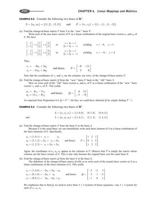
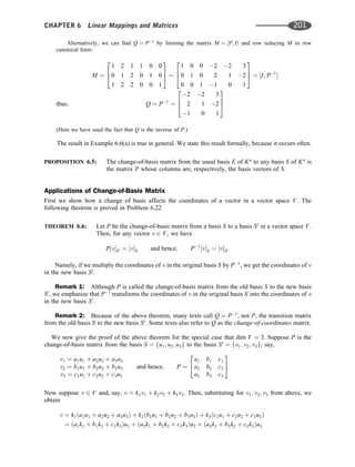
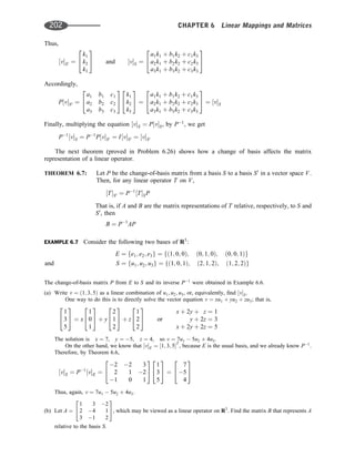
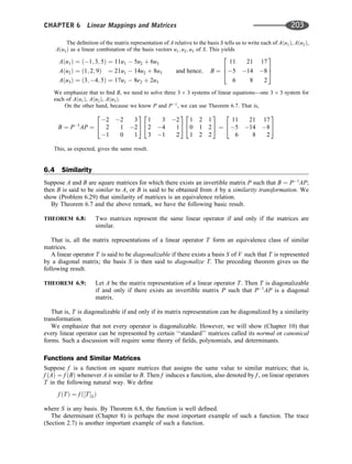
![EXAMPLE 6.8 Consider the following linear operator F and bases E and S of R2
:
Fðx; yÞ ¼ ð2x þ 3y; 4x 5yÞ; E ¼ fð1; 0Þ; ð0; 1Þg; S ¼ fð1; 2Þ; ð2; 5Þg
By Example 6.1, the matrix representations of F relative to the bases E and S are, respectively,
A ¼
2 3
4 5
and B ¼
52 129
22 55
Using matrix A, we have
(i) Determinant of F ¼ detðAÞ ¼ 10 12 ¼ 22; (ii) Trace of F ¼ trðAÞ ¼ 2 5 ¼ 3:
On the other hand, using matrix B, we have
(i) Determinant of F ¼ detðBÞ ¼ 2860 þ 2838 ¼ 22; (ii) Trace of F ¼ trðBÞ ¼ 52 55 ¼ 3.
As expected, both matrices yield the same result.
6.5 Matrices and General Linear Mappings
Last, we consider the general case of linear mappings from one vector space into another. Suppose V and
U are vector spaces over the same field K and, say, dim V ¼ m and dim U ¼ n. Furthermore, suppose
S ¼ fv1; v2; . . . ; vmg and S0
¼ fu1; u2; . . . ; ung
are arbitrary but fixed bases, respectively, of V and U.
Suppose F: V ! U is a linear mapping. Then the vectors Fðv1Þ, Fðv2Þ; . . . ; FðvmÞ belong to U,
and so each is a linear combination of the basis vectors in S0
; say,
Fðv1Þ ¼ a11u1 þ a12u2 þ þ a1nun
Fðv2Þ ¼ a21u1 þ a22u2 þ þ a2nun
:::::::::::::::::::::::::::::::::::::::::::::::::::::::
FðvmÞ ¼ am1u1 þ am2u2 þ þ amnun
DEFINITION: The transpose of the above matrix of coefficients, denoted by mS;S0 ðFÞ or ½FS;S0 , is
called the matrix representation of F relative to the bases S and S0
. [We will use the
simple notation mðFÞ and ½F when the bases are understood.]
The following theorem is analogous to Theorem 6.1 for linear operators (Problem 6.67).
THEOREM 6.10: For any vector v 2 V, ½FS;S0 ½vS ¼ ½FðvÞS0 .
That is, multiplying the coordinates of v in the basis S of V by ½F, we obtain the coordinates of FðvÞ
in the basis S0
of U.
Recall that for any vector spaces V and U, the collection of all linear mappings from V into U is a
vector space and is denoted by HomðV; UÞ. The following theorem is analogous to Theorem 6.2 for linear
operators, where now we let M ¼ Mm;n denote the vector space of all m n matrices (Problem 6.67).
THEOREM 6.11: The mapping m: HomðV; UÞ ! M defined by mðFÞ ¼ ½F is a vector space
isomorphism. That is, for any F; G 2 HomðV; UÞ and any scalar k,
(i) mðF þ GÞ ¼ mðFÞ þ mðGÞ or ½F þ G ¼ ½F þ ½G
(ii) mðkFÞ ¼ kmðFÞ or ½kF ¼ k½F
(iii) m is bijective (one-to-one and onto).
204 CHAPTER 6 Linear Mappings and Matrices](https://image.slidesharecdn.com/linearalgebra4thedition-231030053714-df1faee2/85/Linear_Algebra-_4th_Edition-pdf-211-320.jpg)
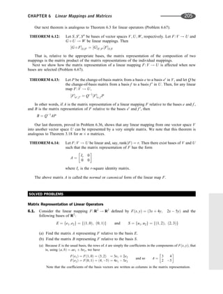
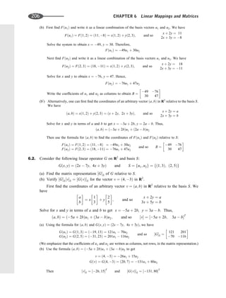
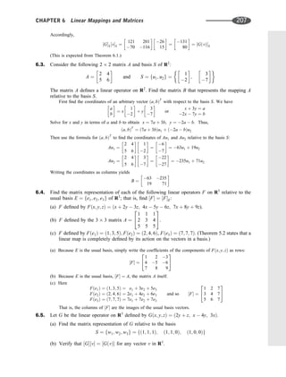
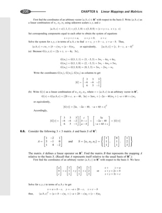
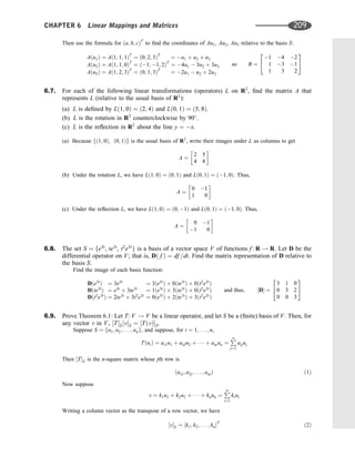
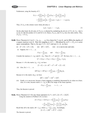
![6.12. Let A be the matrix representation of a linear operator T. Prove that, for any polynomial f ðtÞ, we
have that f ðAÞ is the matrix representation of f ðTÞ. [Thus, f ðTÞ ¼ 0 if and only if f ðAÞ ¼ 0.]
Let f be the mapping that sends an operator T into its matrix representation A. We need to prove that
fð f ðTÞÞ ¼ f ðAÞ. Suppose f ðtÞ ¼ antn
þ þ a1t þ a0. The proof is by induction on n, the degree of f ðtÞ.
Suppose n ¼ 0. Recall that fðI0
Þ ¼ I, where I0
is the identity mapping and I is the identity matrix. Thus,
fð f ðTÞÞ ¼ fða0I0
Þ ¼ a0fðI0
Þ ¼ a0I ¼ f ðAÞ
and so the theorem holds for n ¼ 0.
Now assume the theorem holds for polynomials of degree less than n. Then, because f is an algebra
isomorphism,
fð f ðTÞÞ ¼ fðanTn
þ an1Tn1
þ þ a1T þ a0I0
Þ
¼ anfðTÞfðTn1
Þ þ fðan1Tn1
þ þ a1T þ a0I0
Þ
¼ anAAn1
þ ðan1An1
þ þ a1A þ a0IÞ ¼ f ðAÞ
and the theorem is proved.
Change of Basis
The coordinate vector ½vS in this section will always denote a column vector; that is,
½vS ¼ ½a1; a2; . . . ; anT
6.13. Consider the following bases of R2
:
E ¼ fe1; e2g ¼ fð1; 0Þ; ð0; 1Þg and S ¼ fu1; u2g ¼ fð1; 3Þ; ð1; 4Þg
(a) Find the change-of-basis matrix P from the usual basis E to S.
(b) Find the change-of-basis matrix Q from S back to E.
(c) Find the coordinate vector ½v of v ¼ ð5; 3Þ relative to S.
(a) Because E is the usual basis, simply write the basis vectors in S as columns: P ¼
1 1
3 4
(b) Method 1. Use the definition of the change-of-basis matrix. That is, express each vector in E as a
linear combination of the vectors in S. We do this by first finding the coordinates of an arbitrary vector
v ¼ ða; bÞ relative to S. We have
ða; bÞ ¼ xð1; 3Þ þ yð1; 4Þ ¼ ðx þ y; 3x þ 4yÞ or
x þ y ¼ a
3x þ 4y ¼ b
Solve for x and y to obtain x ¼ 4a b, y ¼ 3a þ b. Thus,
v ¼ ð4a bÞu1 þ ð3a þ bÞu2 and ½vS ¼ ½ða; bÞS ¼ ½4a b; 3a þ bT
Using the above formula for ½vS and writing the coordinates of the ei as columns yields
e1 ¼ ð1; 0Þ ¼ 4u1 3u2
e2 ¼ ð0; 1Þ ¼ u1 þ u2
and Q ¼
4 1
3 1
Method 2. Because Q ¼ P1
; find P1
, say by using the formula for the inverse of a 2 2 matrix.
Thus,
P1
¼
4 1
3 1
(c) Method 1. Write v as a linear combination of the vectors in S, say by using the above formula for
v ¼ ða; bÞ. We have v ¼ ð5; 3Þ ¼ 23u1 18u2; and so ½vS ¼ ½23; 18T
.
Method 2. Use, from Theorem 6.6, the fact that ½vS ¼ P1
½vE and the fact that ½vE ¼ ½5; 3T
:
½vS ¼ P1
½vE ¼
4 1
3 1
5
3
¼
23
18
CHAPTER 6 Linear Mappings and Matrices 211](https://image.slidesharecdn.com/linearalgebra4thedition-231030053714-df1faee2/85/Linear_Algebra-_4th_Edition-pdf-218-320.jpg)
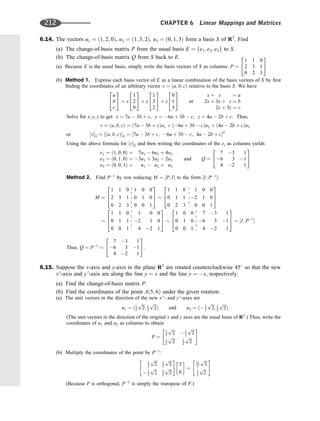
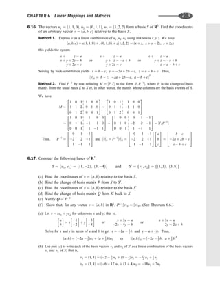
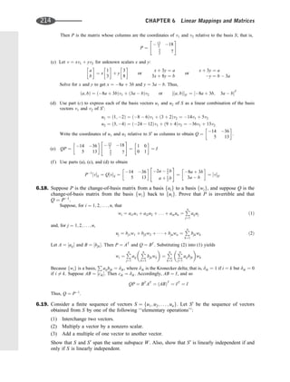
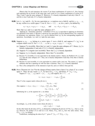
![Linear Operators and Change of Basis
6.23. Consider the linear transformation F on R2
defined by Fðx; yÞ ¼ ð5x y; 2x þ yÞ and the
following bases of R2
:
E ¼ fe1; e2g ¼ fð1; 0Þ; ð0; 1Þg and S ¼ fu1; u2g ¼ fð1; 4Þ; ð2; 7Þg
(a) Find the change-of-basis matrix P from E to S and the change-of-basis matrix Q from S back
to E.
(b) Find the matrix A that represents F in the basis E.
(c) Find the matrix B that represents F in the basis S.
(a) Because E is the usual basis, simply write the vectors in S as columns to obtain the change-of-basis
matrix P. Recall, also, that Q ¼ P1
. Thus,
P ¼
1 2
4 7
and Q ¼ P1
¼
7 2
4 1
(b) Write the coefficients of x and y in Fðx; yÞ ¼ ð5x y; 2x þ yÞ as rows to get
A ¼
5 1
2 1
(c) Method 1. Find the coordinates of Fðu1Þ and Fðu2Þ relative to the basis S. This may be done by first
finding the coordinates of an arbitrary vector ða; bÞ in R2
relative to the basis S. We have
ða; bÞ ¼ xð1; 4Þ þ yð2; 7Þ ¼ ðx þ 2y; 4x þ 7yÞ; and so
x þ 2y ¼ a
4x þ 7y ¼ b
Solve for x and y in terms of a and b to get x ¼ 7a þ 2b, y ¼ 4a b. Then
ða; bÞ ¼ ð7a þ 2bÞu1 þ ð4a bÞu2
Now use the formula for ða; bÞ to obtain
Fðu1Þ ¼ Fð1; 4Þ ¼ ð1; 6Þ ¼ 5u1 2u2
Fðu2Þ ¼ Fð2; 7Þ ¼ ð3; 11Þ ¼ u1 þ u2
and so B ¼
5 1
2 1
Method 2. By Theorem 6.7, B ¼ P1
AP. Thus,
B ¼ P1
AP ¼
7 2
4 1
5 1
2 1
1 2
4 7
¼
5 1
2 1
6.24. Let A ¼
2 3
4 1
. Find the matrix B that represents the linear operator A relative to the basis
S ¼ fu1; u2g ¼ f½1; 3T
; ½2; 5T
g. [Recall A defines a linear operator A: R2
! R2
relative to the
usual basis E of R2
].
Method 1. Find the coordinates of Aðu1Þ and Aðu2Þ relative to the basis S by first finding the coordinates
of an arbitrary vector ½a; bT
in R2
relative to the basis S. By Problem 6.2,
½a; bT
¼ ð5a þ 2bÞu1 þ ð3a bÞu2
Using the formula for ½a; bT
, we obtain
Aðu1Þ ¼
2 3
4 1
1
3
¼
11
1
¼ 53u1 þ 32u2
and Aðu2Þ ¼
2 3
4 1
2
5
¼
19
3
¼ 89u1 þ 54u2
Thus; B ¼
53 89
32 54
Method 2. Use B ¼ P1
AP, where P is the change-of-basis matrix from the usual basis E to S. Thus,
simply write the vectors in S (as columns) to obtain the change-of-basis matrix P and then use the formula
216 CHAPTER 6 Linear Mappings and Matrices](https://image.slidesharecdn.com/linearalgebra4thedition-231030053714-df1faee2/85/Linear_Algebra-_4th_Edition-pdf-223-320.jpg)
![for P1
. This gives
P ¼
1 2
3 5
and P1
¼
5 2
3 1
Then B ¼ P1
AP ¼
1 2
3 5
2 3
4 1
5 2
3 1
¼
53 89
32 54
6.25. Let A ¼
1 3 1
2 5 4
1 2 2
2
4
3
5: Find the matrix B that represents the linear operator A relative to the
basis
S ¼ fu1; u2; u3g ¼ f½1; 1; 0T
; ½0; 1; 1T
; ½1; 2; 2T
g
[Recall A that defines a linear operator A: R3
! R3
relative to the usual basis E of R3
.]
Method 1. Find the coordinates of Aðu1Þ, Aðu2Þ, Aðu3Þ relative to the basis S by first finding the
coordinates of an arbitrary vector v ¼ ða; b; cÞ in R3
relative to the basis S. By Problem 6.16,
½vS ¼ ðb cÞu1 þ ð2a þ 2b cÞu2 þ ða b þ cÞu3
Using this formula for ½a; b; cT
, we obtain
Aðu1Þ ¼ ½4; 7; 1T
¼ 8u1 þ 7u2 5u3; Aðu2Þ ¼ ½4; 1; 0T
¼ u1 6u2 þ 3u3
Aðu3Þ ¼ ½9; 4; 1T
¼ 3u1 11u2 þ 6u3
Writing the coefficients of u1; u2; u3 as columns yields
B ¼
8 1 3
7 6 11
5 3 6
2
4
3
5
Method 2. Use B ¼ P1
AP, where P is the change-of-basis matrix from the usual basis E to S. The matrix
P (whose columns are simply the vectors in S) and P1
appear in Problem 6.16. Thus,
B ¼ P1
AP ¼
0 1 1
2 2 1
1 1 1
2
4
3
5
1 3 1
2 5 4
1 2 2
2
4
3
5
1 0 1
1 1 2
0 1 2
2
4
3
5 ¼
8 1 3
7 6 11
5 3 6
2
4
3
5
6.26. Prove Theorem 6.7: Let P be the change-of-basis matrix from a basis S to a basis S0
in a vector
space V. Then, for any linear operator T on V, ½TS0 ¼ P1
½TSP.
Let v be a vector in V. Then, by Theorem 6.6, P½vS0 ¼ ½vS. Therefore,
P1
½TSP½vS0 ¼ P1
½TS½vS ¼ P1
½TðvÞS ¼ ½TðvÞS0
But ½TS0 ½vS0 ¼ ½TðvÞS0 . Hence,
P1
½TSP½vS0 ¼ ½TS0 ½vS0
Because the mapping v 7! ½vS0 is onto Kn
, we have P1
½TSPX ¼ ½TS0 X for every X 2 Kn
. Thus,
P1
½TSP ¼ ½TS0 , as claimed.
Similarity of Matrices
6.27. Let A ¼
4 2
3 6
and P ¼
1 2
3 4
.
(a) Find B ¼ P1
AP. (b) Verify trðBÞ ¼ trðAÞ: (c) Verify detðBÞ ¼ detðAÞ:
(a) First find P1
using the formula for the inverse of a 2 2 matrix. We have
P1
¼
2 1
3
2 1
2
#
CHAPTER 6 Linear Mappings and Matrices 217](https://image.slidesharecdn.com/linearalgebra4thedition-231030053714-df1faee2/85/Linear_Algebra-_4th_Edition-pdf-224-320.jpg)
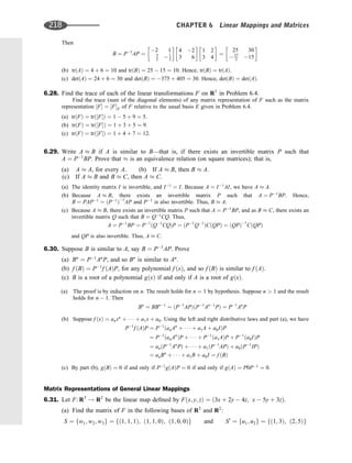
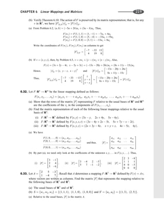
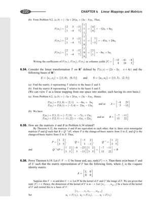
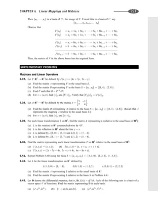
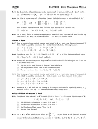
![6.65. Let F: R3
! R2
be defined by Fðx; y; zÞ ¼ ð2x þ y z; 3x 2y þ 4zÞ.
(a) Find the matrix A representing F relative to the bases
S ¼ fð1; 1; 1Þ; ð1; 1; 0Þ; ð1; 0; 0Þg and S0
¼ ð1; 3Þ; ð1; 4Þg
(b) Verify that, for any v ¼ ða; b; cÞ in R3
, A½vS ¼ ½FðvÞS0 .
6.66. Let S and S0
be bases of V, and let 1V be the identity mapping on V. Show that the matrix A representing
1V relative to the bases S and S0
is the inverse of the change-of-basis matrix P from S to S0
; that is,
A ¼ P1
.
6.67. Prove (a) Theorem 6.10, (b) Theorem 6.11, (c) Theorem 6.12, (d) Theorem 6.13. [Hint: See the proofs
of the analogous Theorems 6.1 (Problem 6.9), 6.2 (Problem 6.10), 6.3 (Problem 6.11), and 6.7
(Problem 6.26).]
Miscellaneous Problems
6.68. Suppose F: V ! V is linear. A subspace W of V is said to be invariant under F if FðWÞ W. Suppose W is
invariant under F and dim W ¼ r. Show that F has a block triangular matrix representation M ¼
A B
0 C
where A is an r r submatrix.
6.69. Suppose V ¼ U þ W, and suppose U and V are each invariant under a linear operator F: V ! V. Also,
suppose dim U ¼ r and dim W ¼ S. Show that F has a block diagonal matrix representation M ¼
A 0
0 B
where A and B are r r and s s submatrices.
6.70. Two linear operators F and G on V are said to be similar if there exists an invertible linear operator T on V
such that G ¼ T1
F T. Prove
(a) F and G are similar if and only if, for any basis S of V, ½FS and ½GS are similar matrices.
(b) If F is diagonalizable (similar to a diagonal matrix), then any similar matrix G is also diagonalizable.
ANSWERS TO SUPPLEMENTARY PROBLEMS
Notation: M ¼ ½R1; R2; . . . represents a matrix M with rows R1; R2; . . . :
6.37. (a) A ¼ ½4; 5; 2; 1; (b) B ¼ ½220; 487; 98; 217; (c) P ¼ ½1; 2; 4; 9;
(d) ½vS ¼ ½9a 2b; 4a þ bT
and ½FðvÞS ¼ ½32a þ 47b; 14a 21bT
6.38. (a) B ¼ ½6; 28; 4; 15;
(b) ½vS ¼ ½4a b; 3
2 a þ 1
2 bT
and ½AðvÞS ¼ ½18a 8b; 1
2 ð13a þ 7bÞ
6.39. (a) ½
ffiffiffi
2
p
;
ffiffiffi
2
p
;
ffiffiffi
2
p
;
ffiffiffi
2
p
; (b) ½0; 1; 1; 0; (c) ½3; 7; 5; 2;
(d) ½1; 2; 18; 11
6.40. (a) ½1; 0; 0; 0; 1; 0; 0; 0; 0; (b) ½0; 0; 1; 0; 1; 1; 1; 1; 1;
(c) ½2; 7; 4; 3; 1; 4; 6; 8; 1
6.41. (a) ½1; 3; 5; 0; 5; 10; 0; 3; 6; (b) ½0; 1; 2; 1; 2; 3; 1; 0; 0;
(c) ½15; 65; 104; 49; 219; 351; 29; 130; 208
6.42. (a) ½1; 1; 2; 1; 3; 2; 1; 5; 2; (b) ½0; 2; 14; 22; 0; 5; 8
6.43. (a) ½1; 0; 0; 0; 2; 1; 0; 0; 2; (b) ½0; 1; 0; 0; 0; 0; 0; 0; 3; 0; 0; 3; 0;
(c) ½5; 1; 0; 0; 5; 2; 0; 0; 5
224 CHAPTER 6 Linear Mappings and Matrices](https://image.slidesharecdn.com/linearalgebra4thedition-231030053714-df1faee2/85/Linear_Algebra-_4th_Edition-pdf-231-320.jpg)
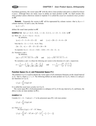
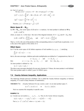
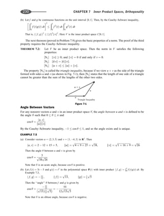
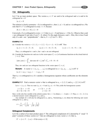
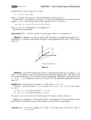
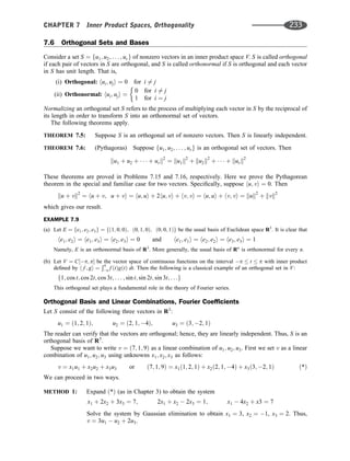
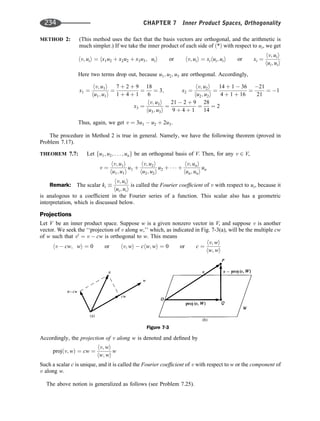
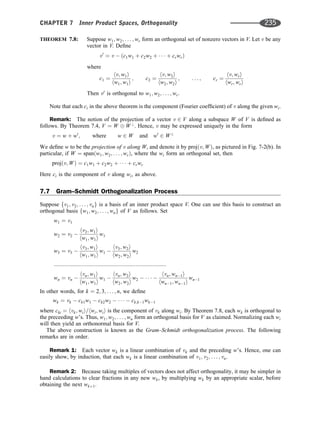
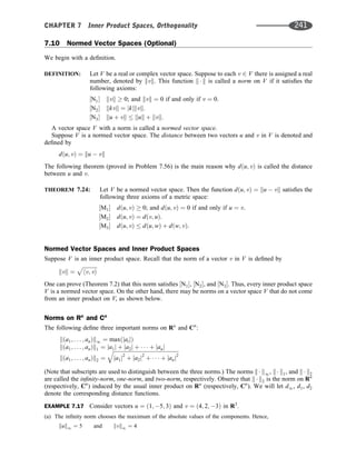
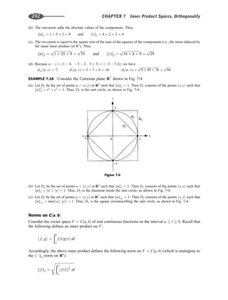
![(a) Take the inner product of each term on the left with each term on the right:
h5u1 þ 8u2; 6v1 7v2i ¼ h5u1; 6v1i þ h5u1; 7v2i þ h8u2; 6v1i þ h8u2; 7v2i
¼ 30hu1; v1i 35hu1; v2i þ 48hu2; v1i 56hu2; v2i
[Remark: Observe the similarity between the above expansion and the expansion (5a–8b)(6c–7d ) in
ordinary algebra.]
(b) h3u þ 5v; 4u 6vi ¼ 12hu; ui 18hu; vi þ 20hv; ui 30hv; vi
¼ 12hu; ui þ 2hu; vi 30hv; vi
(c) k2u 3vk2
¼ h2u 3v; 2u 3vi ¼ 4hu; ui 6hu; vi 6hv; ui þ 9hv; vi
¼ 4kuk2
12ðu; vÞ þ 9kvk2
7.2. Consider vectors u ¼ ð1; 2; 4Þ; v ¼ ð2; 3; 5Þ; w ¼ ð4; 2; 3Þ in R3
. Find
(a) u v, (b) u w; (c) v w, (d) ðu þ vÞ w, (e) kuk, (f ) kvk.
(a) Multiply corresponding components and add to get u v ¼ 2 6 þ 20 ¼ 16:
(b) u w ¼ 4 þ 4 12 ¼ 4.
(c) v w ¼ 8 6 15 ¼ 13.
(d) First find u þ v ¼ ð3; 1; 9Þ. Then ðu þ vÞ w ¼ 12 2 27 ¼ 17. Alternatively, using ½I1,
ðu þ vÞ w ¼ u w þ v w ¼ 4 13 ¼ 17.
(e) First find kuk2
by squaring the components of u and adding:
kuk2
¼ 12
þ 22
þ 42
¼ 1 þ 4 þ 16 ¼ 21; and so kuk ¼
ffiffiffiffiffi
21
p
(f ) kvk2
¼ 4 þ 9 þ 25 ¼ 38, and so kvk ¼
ffiffiffiffiffi
38
p
.
7.3. Verify that the following defines an inner product in R2
:
hu; vi ¼ x1y1 x1y2 x2y1 þ 3x2y2; where u ¼ ðx1; x2Þ; v ¼ ðy1; y2Þ
We argue via matrices. We can write hu; vi in matrix notation as follows:
hu; vi ¼ uT
Av ¼ ½x1; x2
1 1
1 3
y1
y2
Because A is real and symmetric, we need only show that A is positive definite. The diagonal elements 1 and
3 are positive, and the determinant kAk ¼ 3 1 ¼ 2 is positive. Thus, by Theorem 7.14, A is positive
definite. Accordingly, by Theorem 7.15, hu; vi is an inner product.
7.4. Consider the vectors u ¼ ð1; 5Þ and v ¼ ð3; 4Þ in R2
. Find
(a) hu; vi with respect to the usual inner product in R2
.
(b) hu; vi with respect to the inner product in R2
in Problem 7.3.
(c) kvk using the usual inner product in R2
.
(d) kvk using the inner product in R2
in Problem 7.3.
(a) hu; vi ¼ 3 þ 20 ¼ 23.
(b) hu; vi ¼ 1 3 1 4 5 3 þ 3 5 4 ¼ 3 4 15 þ 60 ¼ 44.
(c) kvk2
¼ hv; vi ¼ hð3; 4Þ; ð3; 4Þi ¼ 9 þ 16 ¼ 25; hence, jvk ¼ 5.
(d) kvk2
¼ hv; vi ¼ hð3; 4Þ; ð3; 4Þi ¼ 9 12 12 þ 48 ¼ 33; hence, kvk ¼
ffiffiffiffiffi
33
p
.
7.5. Consider the following polynomials in PðtÞ with the inner product h f ; gi ¼
Ð1
0 f ðtÞgðtÞ dt:
f ðtÞ ¼ t þ 2; gðtÞ ¼ 3t 2; hðtÞ ¼ t2
2t 3
(a) Find h f ; gi and h f ; hi.
(b) Find k f k and kgk.
(c) Normalize f and g.
244 CHAPTER 7 Inner Product Spaces, Orthogonality](https://image.slidesharecdn.com/linearalgebra4thedition-231030053714-df1faee2/85/Linear_Algebra-_4th_Edition-pdf-251-320.jpg)
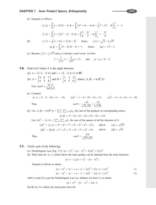
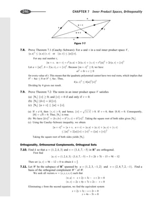
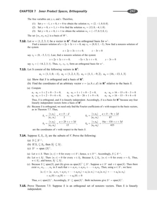
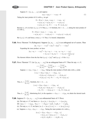
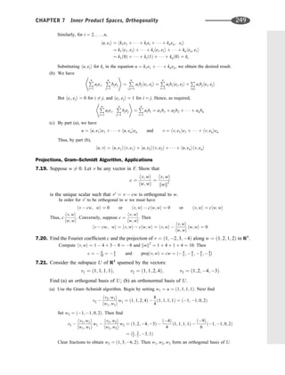
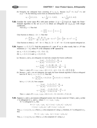
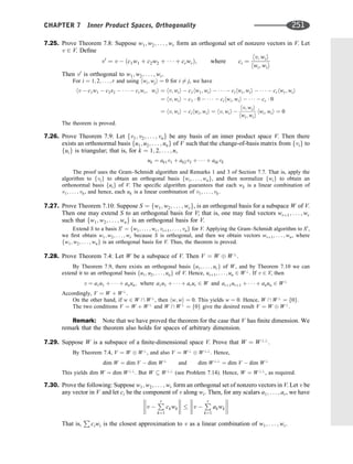
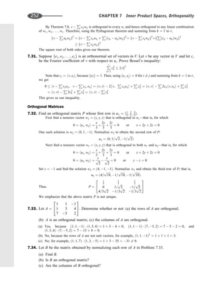
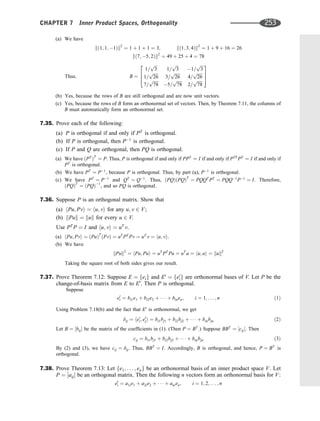
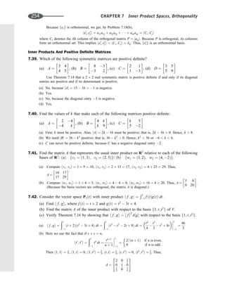
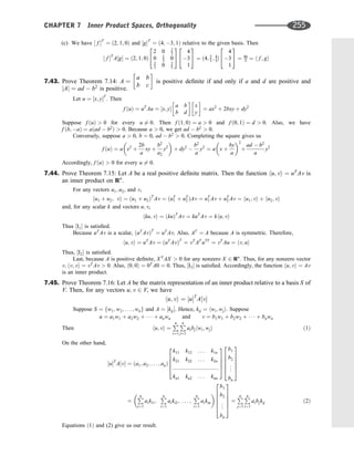
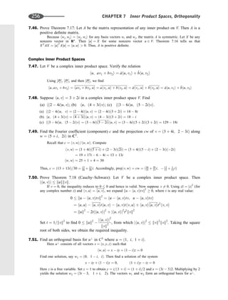
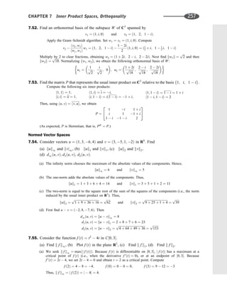
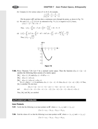
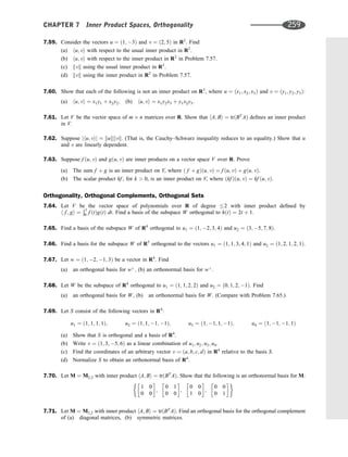
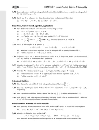
![7.85. Find the matrix C that represents the usual basis on R3
relative to the basis S of R3
consisting of the vectors
u1 ¼ ð1; 1; 1Þ, u2 ¼ ð1; 2; 1Þ, u3 ¼ ð1; 1; 3Þ.
7.86. Let V ¼ P2ðtÞ with inner product h f ; gi ¼
Ð1
0 f ðtÞgðtÞ dt.
(a) Find h f ; gi, where f ðtÞ ¼ t þ 2 and gðtÞ ¼ t2
3t þ 4.
(b) Find the matrix A of the inner product with respect to the basis f1; t; t2
g of V.
(c) Verify Theorem 7.16 that h f ; gi ¼ ½ f T
A½g with respect to the basis f1; t; t2
g.
7.87. Determine which of the following matrices are positive definite:
(a)
1 3
3 5
, (b)
3 4
4 7
, (c)
4 2
2 1
, (d)
6 7
7 9
.
7.88. Suppose A and B are positive definite matrices. Show that:
(a) A þ B is positive definite and (b) kA is positive definite for k 0.
7.89. Suppose B is a real nonsingular matrix. Show that: (a) BT
B is symmetric and (b) BT
B is positive definite.
Complex Inner Product Spaces
7.90. Verify that
ha1u1 þ a2u2 b1v1 þ b2v2i ¼ a1
b1hu1; v1i þ a1
b2hu1; v2i þ a2
b1hu2; v1i þ a2
b2hu2; v2i
More generally, prove that h
Pm
i¼1 aiui;
Pn
j¼1 bjvji ¼
P
i;j ai
bjhui; vii.
7.91. Consider u ¼ ð1 þ i; 3; 4 iÞ and v ¼ ð3 4i; 1 þ i; 2iÞ in C3
. Find
(a) hu; vi, (b) hv; ui, (c) kuk, (d) kvk, (e) dðu; vÞ.
7.92. Find the Fourier coefficient c and the projection cw of
(a) u ¼ ð3 þ i; 5 2iÞ along w ¼ ð5 þ i; 1 þ iÞ in C2
,
(b) u ¼ ð1 i; 3i; 1 þ iÞ along w ¼ ð1; 2 i; 3 þ 2iÞ in C3
.
7.93. Let u ¼ ðz1; z2Þ and v ¼ ðw1; w2Þ belong to C2
. Verify that the following is an inner product of C2
:
f ðu; vÞ ¼ z1
w1 þ ð1 þ iÞz1
w2 þ ð1 iÞz2
w1 þ 3z2
w2
7.94. Find an orthogonal basis and an orthonormal basis for the subspace W of C3
spanned by u1 ¼ ð1; i; 1Þ and
u2 ¼ ð1 þ i; 0; 2Þ.
7.95. Let u ¼ ðz1; z2Þ and v ¼ ðw1; w2Þ belong to C2
. For what values of a; b; c; d 2 C is the following an inner
product on C2
?
f ðu; vÞ ¼ az1
w1 þ bz1
w2 þ cz2
w1 þ dz2
w2
7.96. Prove the following form for an inner product in a complex space V:
hu; vi ¼ 1
4 ku þ vk2
1
4 ku vk2
þ 1
4 ku þ ivk2
1
4 ku ivk2
[Compare with Problem 7.7(b).]
7.97. Let V be a real inner product space. Show that
(i) kuk ¼ kvk if and only if hu þ v; u vi ¼ 0;
(ii) ku þ vk2
¼ kuk2
þ kvk2
if and only if hu; vi ¼ 0.
Show by counterexamples that the above statements are not true for, say, C2
.
7.98. Find the matrix P that represents the usual inner product on C3
relative to the basis f1; 1 þ i; 1 2ig.
CHAPTER 7 Inner Product Spaces, Orthogonality 261](https://image.slidesharecdn.com/linearalgebra4thedition-231030053714-df1faee2/85/Linear_Algebra-_4th_Edition-pdf-268-320.jpg)
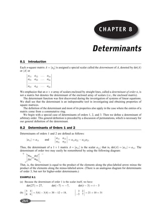
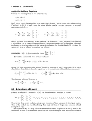
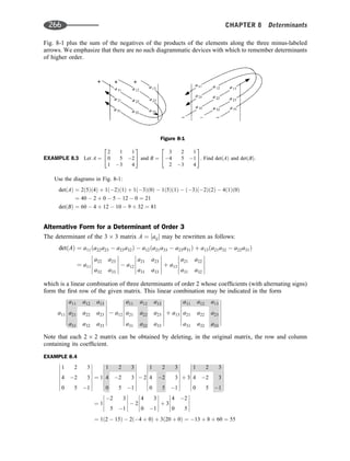
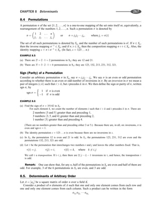
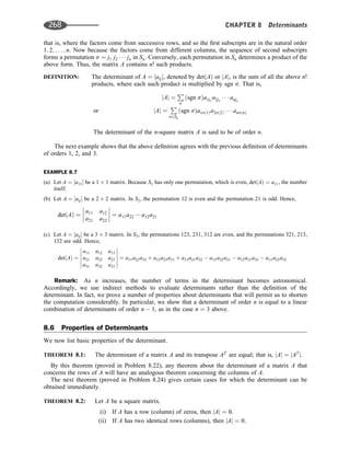
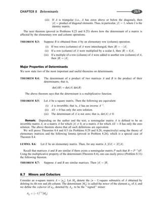
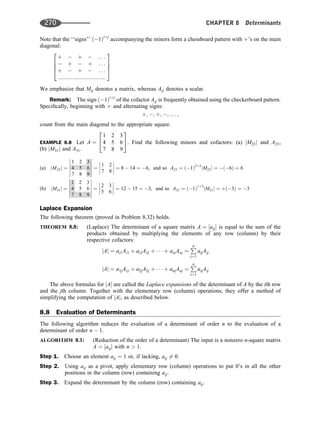
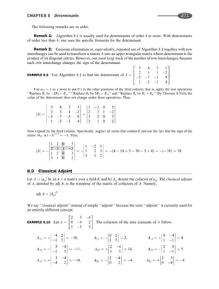
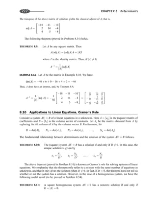
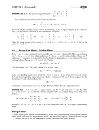
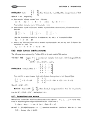
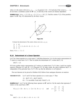
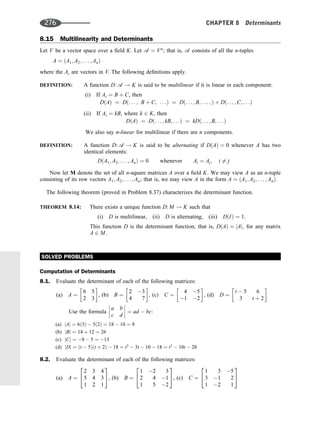
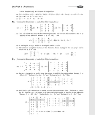
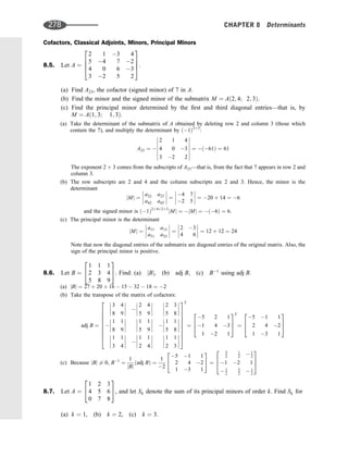
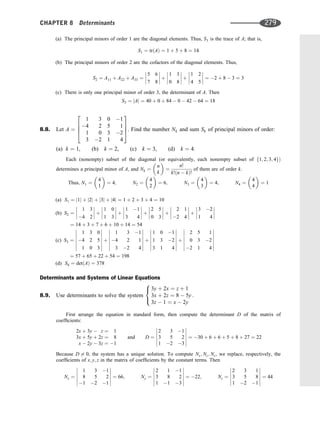
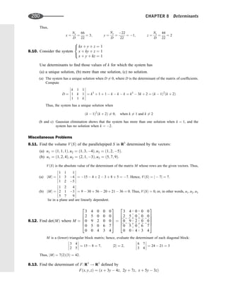
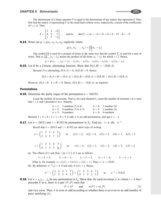
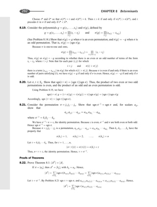
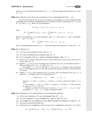
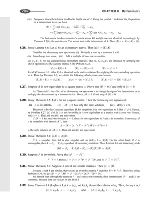
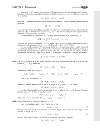
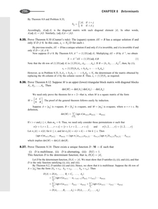
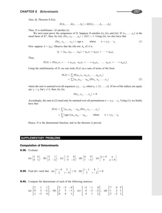
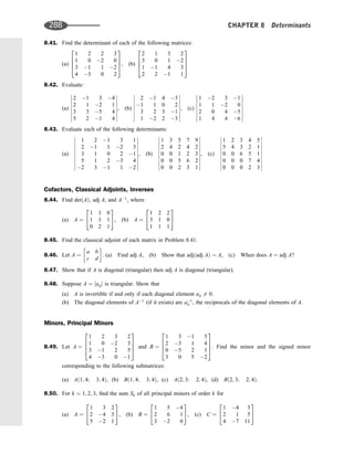
![8.51. For k ¼ 1; 2; 3; 4, find the sum Sk of all principal minors of order k for
(a) A ¼
1 2 3 1
1 2 0 5
0 1 2 2
4 0 1 3
2
6
6
4
3
7
7
5, (b) B ¼
1 2 1 2
0 1 2 3
1 3 0 4
2 7 4 5
2
6
6
4
3
7
7
5
Determinants and Linear Equations
8.52. Solve the following systems by determinants:
(a)
3x þ 5y ¼ 8
4x 2y ¼ 1
, (b)
2x 3y ¼ 1
4x þ 7y ¼ 1
, (c)
ax 2by ¼ c
3ax 5by ¼ 2c
ðab 6¼ 0Þ
8.53. Solve the following systems by determinants:
(a)
2x 5y þ 2z ¼ 2
x þ 2y 4z ¼ 5
3x 4y 6z ¼ 1
8
:
, (b)
2z þ 3 ¼ y þ 3x
x 3z ¼ 2y þ 1
3y þ z ¼ 2 2x
8
:
8.54. Prove Theorem 8.11: The system AX ¼ 0 has a nonzero solution if and only if D ¼ jAj ¼ 0.
Permutations
8.55. Find the parity of the permutations s ¼ 32154, t ¼ 13524, p ¼ 42531 in S5.
8.56. For the permutations in Problem 8.55, find
(a) t s, (b) p s, (c) s1
, (d) t1
.
8.57. Let t 2 Sn: Show that t s runs through Sn as s runs through Sn; that is, Sn ¼ ft s : s 2 Sng:
8.58. Let s 2 Sn have the property that sðnÞ ¼ n. Let s* 2 Sn1 be defined by s*ðxÞ ¼ sðxÞ.
(a) Show that sgn s* ¼ sgn s,
(b) Show that as s runs through Sn, where sðnÞ ¼ n, s* runs through Sn1; that is,
Sn1 ¼ fs* : s 2 Sn; sðnÞ ¼ ng:
8.59. Consider a permutation s ¼ j1 j2 . . . jn. Let feig be the usual basis of Kn
, and let A be the matrix whose ith
row is eji
[i.e., A ¼ ðej1
, ej2
; . . . ; ejn
Þ]. Show that jAj ¼ sgn s.
Determinant of Linear Operators
8.60. Find the determinant of each of the following linear transformations:
(a) T:R2
! R2
defined by Tðx; yÞ ¼ ð2x 9y; 3x 5yÞ,
(b) T:R3
! R3
defined by Tðx; y; zÞ ¼ ð3x 2z; 5y þ 7z; x þ y þ zÞ,
(c) T:R3
! R2
defined by Tðx; y; zÞ ¼ ð2x þ 7y 4z; 4x 6y þ 2zÞ.
8.61. Let D:V ! V be the differential operator; that is, Dð f ðtÞÞ ¼ df =dt. Find detðDÞ if V is the vector space of
functions with the following bases: (a) f1; t; . . . ; t5
g, (b) fet
; e2t
; e3t
g, (c) fsin t; cos tg.
8.62. Prove Theorem 8.13: Let F and G be linear operators on a vector space V. Then
(i) detðF GÞ ¼ detðFÞ detðGÞ, (ii) F is invertible if and only if detðFÞ 6¼ 0.
8.63. Prove (a) detð1V Þ ¼ 1, where 1V is the identity operator, (b) -detðT1
Þ ¼ detðTÞ1
when T is invertible.
CHAPTER 8 Determinants 289](https://image.slidesharecdn.com/linearalgebra4thedition-231030053714-df1faee2/85/Linear_Algebra-_4th_Edition-pdf-296-320.jpg)
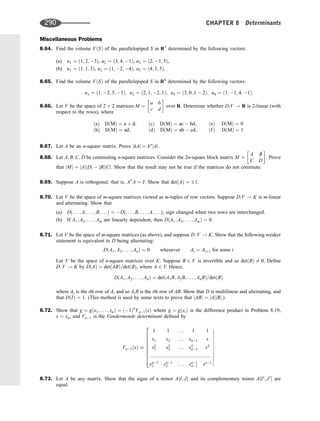
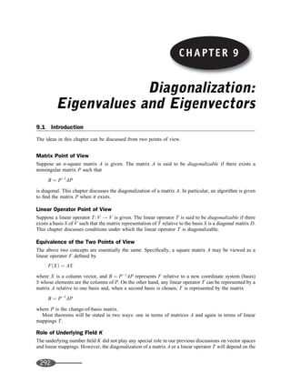
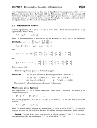
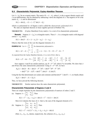
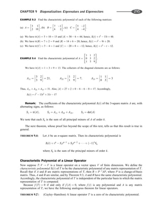
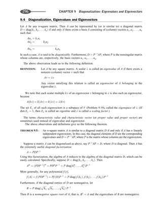
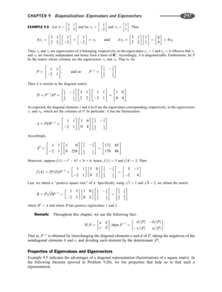
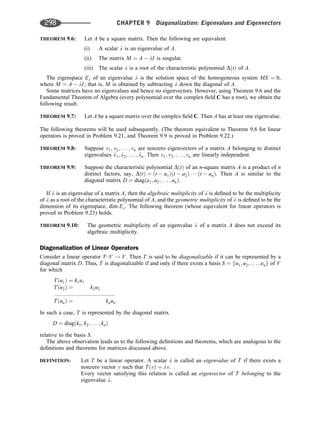
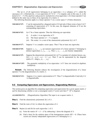
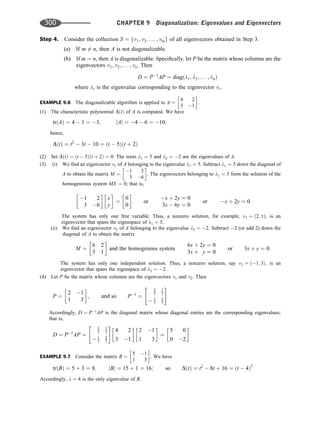
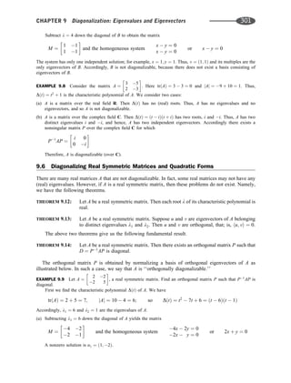
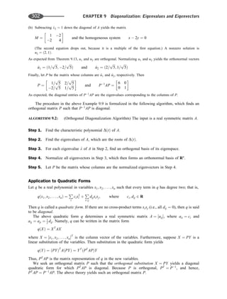
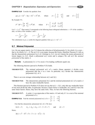
![The minimal polynomial mðtÞ must divide DðtÞ. Also, each irreducible factor of DðtÞ (i.e., t 1 and t 3) must
also be a factor of mðtÞ. Thus, mðtÞ is exactly one of the following:
f ðtÞ ¼ ðt 3Þðt 1Þ or gðtÞ ¼ ðt 3Þðt 1Þ2
We know, by the Cayley–Hamilton theorem, that gðAÞ ¼ DðAÞ ¼ 0. Hence, we need only test f ðtÞ. We have
f ðAÞ ¼ ðA IÞðA 3IÞ ¼
1 2 5
3 6 15
1 2 5
2
4
3
5
1 2 5
3 4 15
1 2 7
2
4
3
5 ¼
0 0 0
0 0 0
0 0 0
2
4
3
5
Thus, f ðtÞ ¼ mðtÞ ¼ ðt 1Þðt 3Þ ¼ t2
4t þ 3 is the minimal polynomial of A.
EXAMPLE 9.12
(a) Consider the following two r-square matrices, where a 6¼ 0:
Jðl; rÞ ¼
l 1 0 . . . 0 0
0 l 1 . . . 0 0
:::::::::::::::::::::::::::::::::
0 0 0 . . . l 1
0 0 0 . . . 0 l
2
6
6
6
6
4
3
7
7
7
7
5
and A ¼
l a 0 . . . 0 0
0 l a . . . 0 0
:::::::::::::::::::::::::::::::::
0 0 0 . . . l a
0 0 0 . . . 0 l
2
6
6
6
6
4
3
7
7
7
7
5
The first matrix, called a Jordan Block, has l’s on the diagonal, 1’s on the superdiagonal (consisting of the
entries above the diagonal entries), and 0’s elsewhere. The second matrix A has l’s on the diagonal, a’s on the
superdiagonal, and 0’s elsewhere. [Thus, A is a generalization of Jðl; rÞ.] One can show that
f ðtÞ ¼ ðt lÞr
is both the characteristic and minimal polynomial of both Jðl; rÞ and A.
(b) Consider an arbitrary monic polynomial:
f ðtÞ ¼ tn
þ an1tn1
þ þ a1t þ a0
Let Cð f Þ be the n-square matrix with 1’s on the subdiagonal (consisting of the entries below the diagonal
entries), the negatives of the coefficients in the last column, and 0’s elsewhere as follows:
Cð f Þ ¼
0 0 . . . 0 a0
1 0 . . . 0 a1
0 1 . . . 0 a2
::::::::::::::::::::::::::::::::::
0 0 . . . 1 an1
2
6
6
6
6
4
3
7
7
7
7
5
Then Cð f Þ is called the companion matrix of the polynomial f ðtÞ. Moreover, the minimal polynomial mðtÞ and
the characteristic polynomial DðtÞ of the companion matrix Cð f Þ are both equal to the original polynomial f ðtÞ.
Minimal Polynomial of a Linear Operator
The minimal polynomial mðtÞ of a linear operator T is defined to be the monic polynomial of lowest
degree for which T is a root. However, for any polynomial f ðtÞ, we have
f ðTÞ ¼ 0 if and only if f ðAÞ ¼ 0
where A is any matrix representation of T. Accordingly, T and A have the same minimal polynomials.
Thus, the above theorems on the minimal polynomial of a matrix also hold for the minimal polynomial of
a linear operator. That is, we have the following theorems.
THEOREM 9.150
: The minimal polynomial mðtÞ of a linear operator T divides every polynomial that
has T as a root. In particular, mðtÞ divides the characteristic polynomial DðtÞ of T.
304 CHAPTER 9 Diagonalization: Eigenvalues and Eigenvectors](https://image.slidesharecdn.com/linearalgebra4thedition-231030053714-df1faee2/85/Linear_Algebra-_4th_Edition-pdf-311-320.jpg)
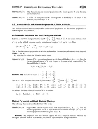
![EXAMPLE 9.14 Find the characteristic polynomal DðtÞ and the minimal polynomial mðtÞ of the block diagonal
matrix:
M ¼
2 5 0 0 0
0 2 0 0 0
0 0 4 2 0
0 0 3 5 0
0 0 0 0 7
2
6
6
6
6
4
3
7
7
7
7
5
¼ diagðA1; A2; A3Þ; where A1 ¼
2 5
0 2
; A2 ¼
4 2
3 5
; A3 ¼ ½7
Then DðtÞ is the product of the characterization polynomials D1ðtÞ, D2ðtÞ, D3ðtÞ of A1; A2; A3, respectively.
One can show that
D1ðtÞ ¼ ðt 2Þ2
; D2ðtÞ ¼ ðt 2Þðt 7Þ; D3ðtÞ ¼ t 7
Thus, DðtÞ ¼ ðt 2Þ3
ðt 7Þ2
. [As expected, deg DðtÞ ¼ 5:
The minimal polynomials m1ðtÞ, m2ðtÞ, m3ðtÞ of the diagonal blocks A1; A2; A3, respectively, are equal to the
characteristic polynomials; that is,
m1ðtÞ ¼ ðt 2Þ2
; m2ðtÞ ¼ ðt 2Þðt 7Þ; m3ðtÞ ¼ t 7
But mðtÞ is equal to the least common multiple of m1ðtÞ; m2ðtÞ; m3ðtÞ. Thus, mðtÞ ¼ ðt 2Þ2
ðt 7Þ.
SOLVED PROBLEMS
Polynomials of Matrices, Characteristic Polynomials
9.1. Let A ¼
1 2
4 5
. Find f ðAÞ, where
ðaÞ f ðtÞ ¼ t2
3t þ 7; ðbÞ f ðtÞ ¼ t2
6t þ 13
First find A2
¼
1 2
4 5
1 2
4 5
¼
7 12
24 17
. Then
(a) f ðAÞ ¼ A2
3A þ 7I ¼
7 12
24 17
þ
3 6
12 15
þ
7 0
0 7
¼
3 6
12 9
(b) f ðAÞ ¼ A2
6A þ 13I ¼
7 12
24 17
þ
6 12
24 30
þ
13 0
0 13
¼
0 0
0 0
[Thus, A is a root of f ðtÞ.]
9.2. Find the characteristic polynomial DðtÞ of each of the following matrices:
(a) A ¼
2 5
4 1
, (b) B ¼
7 3
5 2
, (c) C ¼
3 2
9 3
Use the formula ðtÞ ¼ t2
trðMÞ t þ jMj for a 2 2 matrix M:
(a) trðAÞ ¼ 2 þ 1 ¼ 3, jAj ¼ 2 20 ¼ 18, so DðtÞ ¼ t2
3t 18
(b) trðBÞ ¼ 7 2 ¼ 5, jBj ¼ 14 þ 15 ¼ 1, so DðtÞ ¼ t2
5t þ 1
(c) trðCÞ ¼ 3 3 ¼ 0, jCj ¼ 9 þ 18 ¼ 9, so DðtÞ ¼ t2
þ 9
9.3. Find the characteristic polynomial DðtÞ of each of the following matrices:
(a) A ¼
1 2 3
3 0 4
6 4 5
2
4
3
5, (b) B ¼
1 6 2
3 2 0
0 3 4
2
4
3
5
306 CHAPTER 9 Diagonalization: Eigenvalues and Eigenvectors](https://image.slidesharecdn.com/linearalgebra4thedition-231030053714-df1faee2/85/Linear_Algebra-_4th_Edition-pdf-313-320.jpg)
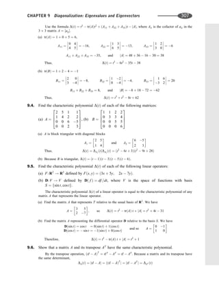
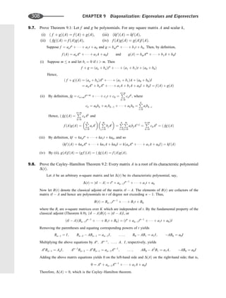
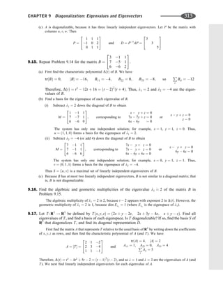
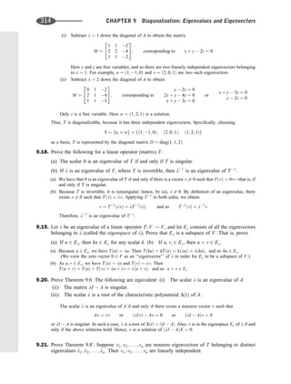
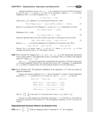
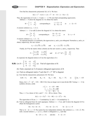
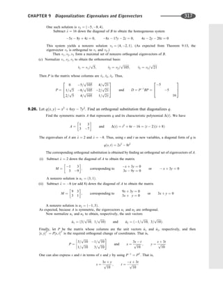
![Minimal Polynomial
9.27. Let A ¼
4 2 2
6 3 4
3 2 3
2
4
3
5 and B ¼
3 2 2
4 4 6
2 3 5
2
4
3
5. The characteristic polynomial of both matrices is
DðtÞ ¼ ðt 2Þðt 1Þ2
. Find the minimal polynomial mðtÞ of each matrix.
The minimal polynomial mðtÞ must divide DðtÞ. Also, each factor of DðtÞ (i.e., t 2 and t 1) must
also be a factor of mðtÞ. Thus, mðtÞ must be exactly one of the following:
f ðtÞ ¼ ðt 2Þðt 1Þ or gðtÞ ¼ ðt 2Þðt 1Þ2
(a) By the Cayley–Hamilton theorem, gðAÞ ¼ DðAÞ ¼ 0, so we need only test f ðtÞ. We have
f ðAÞ ¼ ðA 2IÞðA IÞ ¼
2 2 2
6 5 4
3 2 1
2
4
3
5
3 2 2
6 4 4
3 2 2
2
4
3
5 ¼
0 0 0
0 0 0
0 0 0
2
4
3
5
Thus, mðtÞ ¼ f ðtÞ ¼ ðt 2Þðt 1Þ ¼ t2
3t þ 2 is the minimal polynomial of A.
(b) Again gðBÞ ¼ DðBÞ ¼ 0, so we need only test f ðtÞ. We get
f ðBÞ ¼ ðB 2IÞðB IÞ ¼
1 2 2
4 6 6
2 3 3
2
4
3
5
2 2 2
4 5 6
2 3 4
2
4
3
5 ¼
2 2 2
4 4 4
2 2 2
2
4
3
5 6¼ 0
Thus, mðtÞ 6¼ f ðtÞ. Accordingly, mðtÞ ¼ gðtÞ ¼ ðt 2Þðt 1Þ2
is the minimal polynomial of B. [We
emphasize that we do not need to compute gðBÞ; we know gðBÞ ¼ 0 from the Cayley–Hamilton theorem.]
9.28. Find the minimal polynomial mðtÞ of each of the following matrices:
(a) A ¼
5 1
3 7
, (b) B ¼
1 2 3
0 2 3
0 0 3
2
4
3
5, (c) C ¼
4 1
1 2
(a) The characteristic polynomial of A is DðtÞ ¼ t2
12t þ 32 ¼ ðt 4Þðt 8Þ. Because DðtÞ has distinct
factors, the minimal polynomial mðtÞ ¼ DðtÞ ¼ t2
12t þ 32.
(b) Because B is triangular, its eigenvalues are the diagonal elements 1; 2; 3; and so its characteristic
polynomial is DðtÞ ¼ ðt 1Þðt 2Þðt 3Þ. Because DðtÞ has distinct factors, mðtÞ ¼ DðtÞ.
(c) The characteristic polynomial of C is DðtÞ ¼ t2
6t þ 9 ¼ ðt 3Þ2
. Hence the minimal polynomial of C
is f ðtÞ ¼ t 3 or gðtÞ ¼ ðt 3Þ2
. However, f ðCÞ 6¼ 0; that is, C 3I 6¼ 0. Hence,
mðtÞ ¼ gðtÞ ¼ DðtÞ ¼ ðt 3Þ2
:
9.29. Suppose S ¼ fu1; u2; . . . ; ung is a basis of V, and suppose F and G are linear operators on V such
that ½F has 0’s on and below the diagonal, and ½G has a 6¼ 0 on the superdiagonal and 0’s
elsewhere. That is,
½F ¼
0 a21 a31 . . . an1
0 0 a32 . . . an2
::::::::::::::::::::::::::::::::::::::::
0 0 0 . . . an;n1
0 0 0 . . . 0
2
6
6
6
6
4
3
7
7
7
7
5
; ½G ¼
0 a 0 . . . 0
0 0 a . . . 0
:::::::::::::::::::::::::::
0 0 0 . . . a
0 0 0 . . . 0
2
6
6
6
6
4
3
7
7
7
7
5
Show that (a) Fn
¼ 0, (b) Gn1
6¼ 0, but Gn
¼ 0. (These conditions also hold for ½F and ½G.)
(a) We have Fðu1Þ ¼ 0 and, for r 1, FðurÞ is a linear combination of vectors preceding ur in S. That is,
FðurÞ ¼ ar1u1 þ ar2u2 þ þ ar;r1ur1
318 CHAPTER 9 Diagonalization: Eigenvalues and Eigenvectors](https://image.slidesharecdn.com/linearalgebra4thedition-231030053714-df1faee2/85/Linear_Algebra-_4th_Edition-pdf-325-320.jpg)
![Hence, F2
ðurÞ ¼ FðFðurÞÞ is a linear combination of vectors preceding ur1, and so on. Hence,
Fr
ðurÞ ¼ 0 for each r. Thus, for each r, Fn
ðurÞ ¼ Fnr
ð0Þ ¼ 0, and so Fn
¼ 0, as claimed.
(b) We have Gðu1Þ ¼ 0 and, for each k 1, GðukÞ ¼ auk1. Hence, Gr
ðukÞ ¼ ar
ukr for r k. Because a 6¼ 0,
an1
6¼ 0. Therefore, Gn1
ðunÞ ¼ an1
u1 6¼ 0, and so Gn1
6¼ 0. On the other hand, by (a), Gn
¼ 0.
9.30. Let B be the matrix in Example 9.12(a) that has 1’s on the diagonal, a’s on the superdiagonal,
where a 6¼ 0, and 0’s elsewhere. Show that f ðtÞ ¼ ðt lÞn
is both the characteristic polynomial
DðtÞ and the minimum polynomial mðtÞ of A.
Because A is triangular with l’s on the diagonal, DðtÞ ¼ f ðtÞ ¼ ðt lÞn
is its characteristic polynomial.
Thus, mðtÞ is a power of t l. By Problem 9.29, ðA lIÞr1
6¼ 0. Hence, mðtÞ ¼ DðtÞ ¼ ðt lÞn
.
9.31. Find the characteristic polynomial DðtÞ and minimal polynomial mðtÞ of each matrix:
(a) M ¼
4 1 0 0 0
0 4 1 0 0
0 0 4 0 0
0 0 0 4 1
0 0 0 0 4
2
6
6
6
6
4
3
7
7
7
7
5
, (b) M0
¼
2 7 0 0
0 2 0 0
0 0 1 1
0 0 2 4
2
6
6
4
3
7
7
5
(a) M is block diagonal with diagonal blocks
A ¼
4 1 0
0 4 1
0 0 4
2
4
3
5 and B ¼
4 1
0 4
The characteristic and minimal polynomial of A is f ðtÞ ¼ ðt 4Þ3
and the characteristic and minimal
polynomial of B is gðtÞ ¼ ðt 4Þ2
. Then
DðtÞ ¼ f ðtÞgðtÞ ¼ ðt 4Þ5
but mðtÞ ¼ LCM½ f ðtÞ; gðtÞ ¼ ðt 4Þ3
(where LCM means least common multiple). We emphasize that the exponent in mðtÞ is the size of the
largest block.
(b) Here M0
is block diagonal with diagonal blocks A0
¼
2 7
0 2
and B0
¼
1 1
2 4
The char-
acteristic and minimal polynomial of A0
is f ðtÞ ¼ ðt 2Þ2
. The characteristic polynomial of B0
is
gðtÞ ¼ t2
5t þ 6 ¼ ðt 2Þðt 3Þ, which has distinct factors. Hence, gðtÞ is also the minimal polynomial
of B. Accordingly,
DðtÞ ¼ f ðtÞgðtÞ ¼ ðt 2Þ3
ðt 3Þ but mðtÞ ¼ LCM½ f ðtÞ; gðtÞ ¼ ðt 2Þ2
ðt 3Þ
9.32. Find a matrix A whose minimal polynomial is f ðtÞ ¼ t3
8t2
þ 5t þ 7.
Simply let A ¼
0 0 7
1 0 5
0 1 8
2
4
3
5, the companion matrix of f ðtÞ [defined in Example 9.12(b)].
9.33. Prove Theorem 9.15: The minimal polynomial mðtÞ of a matrix (linear operator) A divides every
polynomial that has A as a zero. In particular (by the Cayley–Hamilton theorem), mðtÞ divides the
characteristic polynomial DðtÞ of A.
Suppose f ðtÞ is a polynomial for which f ðAÞ ¼ 0. By the division algorithm, there exist polynomials
qðtÞ and rðtÞ for which f ðtÞ ¼ mðtÞqðtÞ þ rðtÞ and rðtÞ ¼ 0 or deg rðtÞ deg mðtÞ. Substituting t ¼ A in this
equation, and using that f ðAÞ ¼ 0 and mðAÞ ¼ 0, we obtain rðAÞ ¼ 0. If rðtÞ 6¼ 0, then rðtÞ is a polynomial
of degree less than mðtÞ that has A as a zero. This contradicts the definition of the minimal polynomial. Thus,
rðtÞ ¼ 0, and so f ðtÞ ¼ mðtÞqðtÞ; that is, mðtÞ divides f ðtÞ.
CHAPTER 9 Diagonalization: Eigenvalues and Eigenvectors 319](https://image.slidesharecdn.com/linearalgebra4thedition-231030053714-df1faee2/85/Linear_Algebra-_4th_Edition-pdf-326-320.jpg)
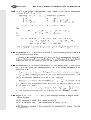
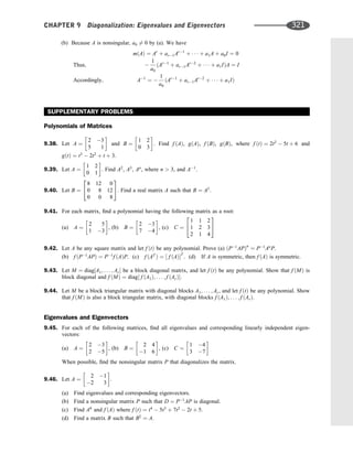
![9.47. Repeat Problem 9.46 for A ¼
5 6
2 2
.
9.48. For each of the following matrices, find all eigenvalues and a maximum set S of linearly independent
eigenvectors:
(a) A ¼
1 3 3
3 5 3
6 6 4
2
4
3
5, (b) B ¼
3 1 1
7 5 1
6 6 2
2
4
3
5, (c) C ¼
1 2 2
1 2 1
1 1 4
2
4
3
5
Which matrices can be diagonalized, and why?
9.49. For each of the following linear operators T: R2
! R2
, find all eigenvalues and a basis for each eigenspace:
(a) Tðx; yÞ ¼ ð3x þ 3y; x þ 5yÞ, (b) Tðx; yÞ ¼ ð3x 13y; x 3yÞ.
9.50. Let A ¼
a b
c d
be a real matrix. Find necessary and sufficient conditions on a; b; c; d so that A is
diagonalizable—that is, so that A has two (real) linearly independent eigenvectors.
9.51. Show that matrices A and AT
have the same eigenvalues. Give an example of a 2 2 matrix A where A and
AT
have different eigenvectors.
9.52. Suppose v is an eigenvector of linear operators F and G. Show that v is also an eigenvector of the linear
operator kF þ k0
G, where k and k0
are scalars.
9.53. Suppose v is an eigenvector of a linear operator T belonging to the eigenvalue l. Prove
(a) For n 0; v is an eigenvector of Tn
belonging to ln
.
(b) f ðlÞ is an eigenvalue of f ðTÞ for any polynomial f ðtÞ.
9.54. Suppose l 6¼ 0 is an eigenvalue of the composition F G of linear operators F and G. Show that l is also an
eigenvalue of the composition G F. [Hint: Show that GðvÞ is an eigenvector of G F.]
9.55. Let E: V ! V be a projection mapping; that is, E2
¼ E. Show that E is diagonalizable and, in fact, can be
represented by the diagonal matrix M ¼
Ir 0
0 0
, where r is the rank of E.
Diagonalizing Real Symmetric Matrices and Quadratic Forms
9.56. For each of the following symmetric matrices A, find an orthogonal matrix P and a diagonal matrix D such
that D ¼ P1
AP:
(a) A ¼
5 4
4 1
, (b) A ¼
4 1
1 4
, (c) A ¼
7 3
3 1
9.57. For each of the following symmetric matrices B, find its eigenvalues, a maximal orthogonal set S of
eigenvectors, and an orthogonal matrix P such that D ¼ P1
BP is diagonal:
(a) B ¼
0 1 1
1 0 1
1 1 0
2
4
3
5, (b) B ¼
2 2 4
2 5 8
4 8 17
2
4
3
5
9.58. Using variables s and t, find an orthogonal substitution that diagonalizes each of the following quadratic
forms:
(a) qðx; yÞ ¼ 4x2
þ 8xy 11y2
, (b) qðx; yÞ ¼ 2x2
6xy þ 10y2
9.59. For each of the following quadratic forms qðx; y; zÞ, find an orthogonal substitution expressing x; y; z in terms
of variables r; s; t, and find qðr; s; tÞ:
(a) qðx; y; zÞ ¼ 5x2
þ 3y2
þ 12xz; (b) qðx; y; zÞ ¼ 3x2
4xy þ 6y2
þ 2xz 4yz þ 3z2
322 CHAPTER 9 Diagonalization: Eigenvalues and Eigenvectors](https://image.slidesharecdn.com/linearalgebra4thedition-231030053714-df1faee2/85/Linear_Algebra-_4th_Edition-pdf-329-320.jpg)
![9.60. Find a real 2 2 symmetric matrix A with eigenvalues:
(a) l ¼ 1 and l ¼ 4 and eigenvector u ¼ ð1; 1Þ belonging to l ¼ 1;
(b) l ¼ 2 and l ¼ 3 and eigenvector u ¼ ð1; 2Þ belonging to l ¼ 2.
In each case, find a matrix B for which B2
¼ A.
Characteristic and Minimal Polynomials
9.61. Find the characteristic and minimal polynomials of each of the following matrices:
(a) A ¼
3 1 1
2 4 2
1 1 3
2
4
3
5, (b) B ¼
3 2 1
3 8 3
3 6 1
2
4
3
5
9.62. Find the characteristic and minimal polynomials of each of the following matrices:
(a) A ¼
2 5 0 0 0
0 2 0 0 0
0 0 4 2 0
0 0 3 5 0
0 0 0 0 7
2
6
6
6
6
4
3
7
7
7
7
5
, (b) B ¼
4 1 0 0 0
1 2 0 0 0
0 0 3 1 0
0 0 0 3 1
0 0 0 0 3
2
6
6
6
6
4
3
7
7
7
7
5
, (c) C ¼
3 2 0 0 0
1 4 0 0 0
0 0 3 1 0
0 0 1 3 0
0 0 0 0 4
2
6
6
6
6
4
3
7
7
7
7
5
9.63. Let A ¼
1 1 0
0 2 0
0 0 1
2
4
3
5 and B ¼
2 0 0
0 2 2
0 0 1
2
4
3
5. Show that A and B have different characteristic polynomials
(and so are not similar) but have the same minimal polynomial. Thus, nonsimilar matrices may have the
same minimal polynomial.
9.64. Let A be an n-square matrix for which Ak
¼ 0 for some k n. Show that An
¼ 0.
9.65. Show that a matrix A and its transpose AT
have the same minimal polynomial.
9.66. Suppose f ðtÞ is an irreducible monic polynomial for which f ðAÞ ¼ 0 for a matrix A. Show that f ðtÞ is the
minimal polynomial of A.
9.67. Show that A is a scalar matrix kI if and only if the minimal polynomial of A is mðtÞ ¼ t k.
9.68. Find a matrix A whose minimal polynomial is (a) t3
5t2
þ 6t þ 8, (b) t4
5t3
2t þ 7t þ 4.
9.69. Let f ðtÞ and gðtÞ be monic polynomials (leading coefficient one) of minimal degree for which A is a root.
Show f ðtÞ ¼ gðtÞ: [Thus, the minimal polynomial of A is unique.]
ANSWERS TO SUPPLEMENTARY PROBLEMS
Notation: M ¼ ½R1; R2; . . . denotes a matrix M with rows R1; R2; . . . :
9.38. f ðAÞ ¼ ½26; 3; 5; 27, gðAÞ ¼ ½40; 39; 65; 27,
f ðBÞ ¼ ½3; 6; 0; 9, gðBÞ ¼ ½3; 12; 0; 15
9.39. A2
¼ ½1; 4; 0; 1, A3
¼ ½1; 6; 0; 1, An
¼ ½1; 2n; 0; 1, A1
¼ ½1; 2; 0; 1
9.40. Let A ¼ ½2; a; b; 0; 2; c; 0; 0; 2. Set B ¼ A3
and then a ¼ 1, b ¼ 1
2, c ¼ 1
CHAPTER 9 Diagonalization: Eigenvalues and Eigenvectors 323](https://image.slidesharecdn.com/linearalgebra4thedition-231030053714-df1faee2/85/Linear_Algebra-_4th_Edition-pdf-330-320.jpg)
![9.41. Find DðtÞ: (a) t2
þ t 11, (b) t2
þ 2t þ 13, (c) t3
7t2
þ 6t 1
9.45. (a) l ¼ 1; u ¼ ð3; 1Þ; l ¼ 4; v ¼ ð1; 2Þ, (b) l ¼ 4; u ¼ ð2; 1Þ,
(c) l ¼ 1; u ¼ ð2; 1Þ; l ¼ 5; v ¼ ð2; 3Þ. Only A and C can be diagonalized; use P ¼ ½u; v.
9.46. (a) l ¼ 1; u ¼ ð1; 1Þ; l ¼ 4; v ¼ ð1; 2Þ,
(b) P ¼ ½u; v,
(c) f ðAÞ ¼ ½3; 1; 2; 1; A8
¼ ½21 846; 21 845; 43 690; 43 691,
(d) B ¼ 4
3 ; 1
3 ; 2
3 ; 5
3
9.47. (a) l ¼ 1; u ¼ ð3; 2Þ; l ¼ 2; v ¼ ð2; 1Þ, (b) P ¼ ½u; v,
(c) f ðAÞ ¼ ½2; 6; 2; 9; A8
¼ ½1021; 1530; 510; 764,
(d) B ¼ ½3 þ 4
ffiffiffi
2
p
; 6 þ 6
ffiffiffi
2
p
; 2 2
ffiffiffi
2
p
; 4 3
ffiffiffi
2
p
9.48. (a) l ¼ 2; u ¼ ð1; 1; 0Þ; v ¼ ð1; 0; 1Þ; l ¼ 4; w ¼ ð1; 1; 2Þ,
(b) l ¼ 2; u ¼ ð1; 1; 0Þ; l ¼ 4; v ¼ ð0; 1; 1Þ,
(c) l ¼ 3; u ¼ ð1; 1; 0Þ; v ¼ ð1; 0; 1Þ; l ¼ 1; w ¼ ð2; 1; 1Þ. Only A and C can be diagonalized; use
P ¼ ½u; v; w:
9.49. (a) l ¼ 2; u ¼ ð3; 1Þ; l ¼ 6; v ¼ ð1; 1Þ, (b) No real eigenvalues
9.50. We need ½trðAÞ2
4½detðAÞ 0 or ða dÞ2
þ 4bc 0.
9.51. A ¼ ½1; 1; 0; 1
9.56. (a) P ¼ ½2; 1; 1; 2=
ffiffiffi
5
p
, D ¼ ½7; 0; 0; 3,
(b) P ¼ ½1; 1; 1; 1=
ffiffiffi
2
p
, D ¼ ½3; 0; 0; 5,
(c) P ¼ ½3; 1; 1; 3=
ffiffiffiffiffi
10
p
, D ¼ ½8; 0; 0; 2
9.57. (a) l ¼ 1; u ¼ ð1; 1; 0Þ; v ¼ ð1; 1; 2Þ; l ¼ 2; w ¼ ð1; 1; 1Þ,
(b) l ¼ 1; u ¼ ð2; 1; 1Þ; v ¼ ð2; 3; 1Þ; l ¼ 22; w ¼ ð1; 2; 4Þ;
Normalize u; v; w, obtaining ^
u; ^
v; ^
w, and set P ¼ ½^
u; ^
v; ^
w. (Remark: u and v are not unique.)
9.58. (a) x ¼ ð4s þ tÞ=
ffiffiffiffiffi
17
p
; y ¼ ðs þ 4tÞ=
ffiffiffiffiffi
17
p
; qðs; tÞ ¼ 5s2
12t2
,
(b) x ¼ ð3s tÞ=
ffiffiffiffiffi
10
p
; y ¼ ðs þ 3tÞ=
ffiffiffiffiffi
10
p
; qðs; tÞ ¼ s2
þ 11t2
9.59. (a) x ¼ ð3s þ 2tÞ=
ffiffiffiffiffi
13
p
; y ¼ r; z ¼ ð2s 3tÞ=
ffiffiffiffiffi
13
p
; qðr; s; tÞ ¼ 3r2
þ 9s2
4t2
,
(b) x ¼ 5Ks þ Lt; y ¼ Jr þ 2Ks 2Lt; z ¼ 2Jr Ks Lt, where J ¼ 1=
ffiffiffi
5
p
, K ¼ 1=
ffiffiffiffiffi
30
p
,
L ¼ 1=
ffiffiffi
6
p
; qðr; s; tÞ ¼ 2r2
þ 2s2
þ 8t2
9.60. (a) A ¼ 1
2 ½5; 3; 3; 5; B ¼ 1
2 ½3; 1; 1; 3,
(b) A ¼ 1
5 ½14; 2; 2; 11, B ¼ 1
5 ½
ffiffiffi
2
p
þ 4
ffiffiffi
3
p
; 2
ffiffiffi
2
p
2
ffiffiffi
3
p
; 2
ffiffiffi
2
p
2
ffiffiffi
3
p
; 4
ffiffiffi
2
p
þ
ffiffiffi
3
p
9.61. (a) DðtÞ ¼ mðtÞ ¼ ðt 2Þ2
ðt 6Þ, (b) DðtÞ ¼ ðt 2Þ2
ðt 6Þ; mðtÞ ¼ ðt 2Þðt 6Þ
9.62. (a) DðtÞ ¼ ðt 2Þ3
ðt 7Þ2
; mðtÞ ¼ ðt 2Þ2
ðt 7Þ,
(b) DðtÞ ¼ ðt 3Þ5
; mðtÞ ¼ ðt 3Þ3
,
(c) DðtÞ ¼ ðt 2Þ2
ðt 4Þ2
ðt 5Þ; mðtÞ ¼ ðt 2Þðt 4Þðt 5Þ
9.68. Let A be the companion matrix [Example 9.12(b)] with last column: (a) ½8; 6; 5T
, (b) ½4; 7; 2; 5T
9.69. Hint: A is a root of hðtÞ ¼ f ðtÞ gðtÞ, where hðtÞ 0 or the degree of hðtÞ is less than the degree of f ðtÞ:
324 CHAPTER 9 Diagonalization: Eigenvalues and Eigenvectors](https://image.slidesharecdn.com/linearalgebra4thedition-231030053714-df1faee2/85/Linear_Algebra-_4th_Edition-pdf-331-320.jpg)
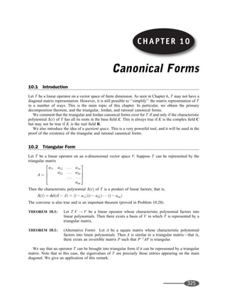
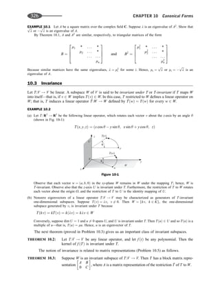
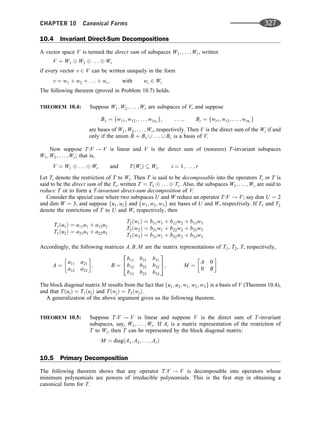
![THEOREM 10.6: (Primary Decomposition Theorem) Let T:V ! V be a linear operator with
minimal polynomial
mðtÞ ¼ f1ðtÞn1
f2ðtÞn2
frðtÞnr
where the fiðtÞ are distinct monic irreducible polynomials. Then V is the direct sum
of T-invariant subspaces W1; . . . ; Wr, where Wi is the kernel of fiðTÞni
. Moreover,
fiðtÞni
is the minimal polynomial of the restriction of T to Wi.
The above polynomials fiðtÞni
are relatively prime. Therefore, the above fundamental theorem
follows (Problem 10.11) from the next two theorems (proved in Problems 10.9 and 10.10, respectively).
THEOREM 10.7: Suppose T:V ! V is linear, and suppose f ðtÞ ¼ gðtÞhðtÞ are polynomials such that
f ðTÞ ¼ 0 and gðtÞ and hðtÞ are relatively prime. Then V is the direct sum of the
T-invariant subspace U and W, where U ¼ Ker gðTÞ and W ¼ Ker hðTÞ.
THEOREM 10.8: In Theorem 10.7, if f ðtÞ is the minimal polynomial of T [and gðtÞ and hðtÞ are
monic], then gðtÞ and hðtÞ are the minimal polynomials of the restrictions of T to U
and W, respectively.
We will also use the primary decomposition theorem to prove the following useful characterization of
diagonalizable operators (see Problem 10.12 for the proof).
THEOREM 10.9: A linear operator T:V ! V is diagonalizable if and only if its minimal polynomial
mðtÞ is a product of distinct linear polynomials.
THEOREM 10.9: (Alternative Form) A matrix A is similar to a diagonal matrix if and only if its
minimal polynomial is a product of distinct linear polynomials.
EXAMPLE 10.3 Suppose A 6¼ I is a square matrix for which A3
¼ I. Determine whether or not A is similar to a
diagonal matrix if A is a matrix over: (i) the real field R, (ii) the complex field C.
Because A3
¼ I, A is a zero of the polynomial f ðtÞ ¼ t3
1 ¼ ðt 1Þðt2
þ t þ 1Þ: The minimal polynomial mðtÞ
of A cannot be t 1, because A 6¼ I. Hence,
mðtÞ ¼ t2
þ t þ 1 or mðtÞ ¼ t3
1
Because neither polynomial is a product of linear polynomials over R, A is not diagonalizable over R. On the
other hand, each of the polynomials is a product of distinct linear polynomials over C. Hence, A is diagonalizable
over C.
10.6 Nilpotent Operators
A linear operator T:V ! V is termed nilpotent if Tn
¼ 0 for some positive integer n; we call k the index
of nilpotency of T if Tk
¼ 0 but Tk1
6¼ 0: Analogously, a square matrix A is termed nilpotent if An
¼ 0
for some positive integer n, and of index k if Ak
¼ 0 but Ak1
6¼ 0. Clearly the minimum polynomial of a
nilpotent operator (matrix) of index k is mðtÞ ¼ tk
; hence, 0 is its only eigenvalue.
EXAMPLE 10.4 The following two r-square matrices will be used throughout the chapter:
N ¼ NðrÞ ¼
0 1 0 . . . 0 0
0 0 1 . . . 0 0
::::::::::::::::::::::::::::::::
0 0 0 . . . 0 1
0 0 0 . . . 0 0
2
6
6
6
6
4
3
7
7
7
7
5
and JðlÞ ¼
l 1 0 . . . 0 0
0 l 1 . . . 0 0
::::::::::::::::::::::::::::::::
0 0 0 . . . l 1
0 0 0 . . . 0 l
2
6
6
6
6
4
3
7
7
7
7
5
328 CHAPTER 10 Canonical Forms](https://image.slidesharecdn.com/linearalgebra4thedition-231030053714-df1faee2/85/Linear_Algebra-_4th_Edition-pdf-335-320.jpg)
![The first matrix N, called a Jordan nilpotent block, consists of 1’s above the diagonal (called the super-
diagonal), and 0’s elsewhere. It is a nilpotent matrix of index r. (The matrix N of order 1 is just the 1 1 zero
matrix [0].)
The second matrix JðlÞ, called a Jordan block belonging to the eigenvalue l, consists of l’s on the diagonal, 1’s
on the superdiagonal, and 0’s elsewhere. Observe that
JðlÞ ¼ lI þ N
In fact, we will prove that any linear operator T can be decomposed into operators, each of which is the sum of a
scalar operator and a nilpotent operator.
The following (proved in Problem 10.16) is a fundamental result on nilpotent operators.
THEOREM 10.10: Let T:V ! V be a nilpotent operator of index k. Then T has a block diagonal
matrix representation in which each diagonal entry is a Jordan nilpotent block N.
There is at least one N of order k, and all other N are of orders k. The number of
N of each possible order is uniquely determined by T. The total number of N of all
orders is equal to the nullity of T.
The proof of Theorem 10.10 shows that the number of N of order i is equal to 2mi miþ1 mi1,
where mi is the nullity of Ti
.
10.7 Jordan Canonical Form
An operator T can be put into Jordan canonical form if its characteristic and minimal polynomials factor
into linear polynomials. This is always true if K is the complex field C. In any case, we can always extend
the base field K to a field in which the characteristic and minimal polynomials do factor into linear
factors; thus, in a broad sense, every operator has a Jordan canonical form. Analogously, every matrix is
similar to a matrix in Jordan canonical form.
The following theorem (proved in Problem 10.18) describes the Jordan canonical form J of a linear
operator T.
THEOREM 10.11: Let T:V ! V be a linear operator whose characteristic and minimal polynomials
are, respectively,
DðtÞ ¼ ðt l1Þn1
ðt lrÞnr
and mðtÞ ¼ ðt l1Þm1
ðt lrÞmr
where the li are distinct scalars. Then T has a block diagonal matrix representa-
tion J in which each diagonal entry is a Jordan block Jij ¼ JðliÞ. For each lij, the
corresponding Jij have the following properties:
(i) There is at least one Jij of order mi; all other Jij are of order mi.
(ii) The sum of the orders of the Jij is ni.
(iii) The number of Jij equals the geometric multiplicity of li.
(iv) The number of Jij of each possible order is uniquely determined by T.
EXAMPLE 10.5 Suppose the characteristic and minimal polynomials of an operator T are, respec-
tively,
DðtÞ ¼ ðt 2Þ4
ðt 5Þ3
and mðtÞ ¼ ðt 2Þ2
ðt 5Þ3
CHAPTER 10 Canonical Forms 329](https://image.slidesharecdn.com/linearalgebra4thedition-231030053714-df1faee2/85/Linear_Algebra-_4th_Edition-pdf-336-320.jpg)
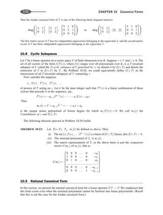
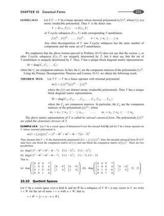
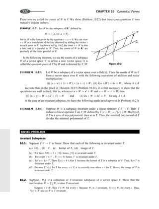
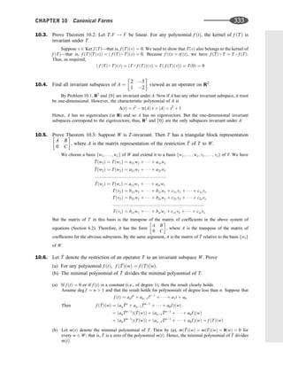
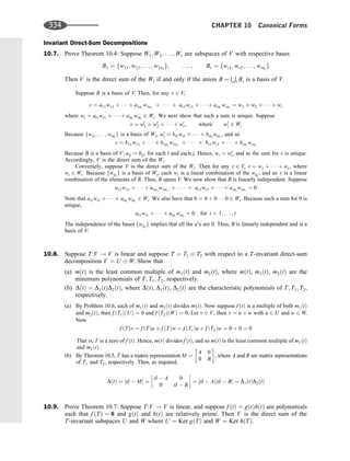
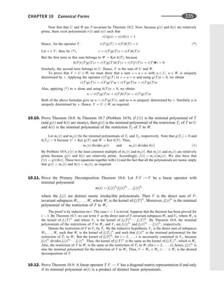
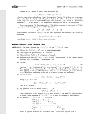
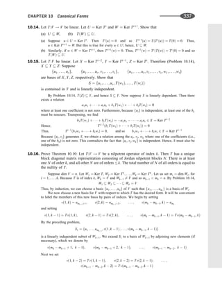
![Again by the preceding problem,
S2 ¼ fu1; . . . ; umks
; vð1; k 2Þ; . . . ; vðmk1 mk2; k 2Þg
is a linearly independent subset of Wk2, which we can extend to a basis of Wk2 by adjoining elements
vðmk1 mk2 þ 1; k 2Þ; vðmk1 mk2 þ 2; k 2Þ; . . . ; vðmk2 mk3; k 2Þ
Continuing in this manner, we get a new basis for V, which for convenient reference we arrange as follows:
vð1; kÞ . . . ; vðmk mk1; kÞ
vð1; k 1Þ; . . . ; vðmk mk1; k 1Þ . . . ; vðmk1 mk2; k 1Þ
:::::::::::::::::::::::::::::::::::::::::::::::::::::::::::::::::::::::
vð1; 2Þ; . . . ; vðmk mk1; 2Þ; . . . ; vðmk1 mk2; 2Þ; . . . ; vðm2 m1; 2Þ
vð1; 1Þ; . . . ; vðmk mk1; 1Þ; . . . ; vðmk1 mk2; 1Þ; . . . ; vðm2 m1; 1Þ; . . . ; vðm1; 1Þ
The bottom row forms a basis of W1, the bottom two rows form a basis of W2, and so forth. But what is
important for us is that T maps each vector into the vector immediately below it in the table or into 0 if the
vector is in the bottom row. That is,
Tvði; jÞ ¼
vði; j 1Þ for j 1
0 for j ¼ 1
Now it is clear [see Problem 10.13(d)] that T will have the desired form if the vði; jÞ are ordered
lexicographically: beginning with vð1; 1Þ and moving up the first column to vð1; kÞ, then jumping to vð2; 1Þ
and moving up the second column as far as possible.
Moreover, there will be exactly mk mk1 diagonal entries of order k: Also, there will be
ðmk1 mk2Þ ðmk mk1Þ ¼ 2mk1 mk mk2 diagonal entries of order k 1
:::::::::::::::::::::::::::::::::::::::::::::::::::::::::::::::::::::::::::::::
2m2 m1 m3 diagonal entries of order 2
2m1 m2 diagonal entries of order 1
as can be read off directly from the table. In particular, because the numbers m1; . . . ; mk are uniquely
determined by T, the number of diagonal entries of each order is uniquely determined by T. Finally, the
identity
m1 ¼ ðmk mk1Þ þ ð2mk1 mk mk2Þ þ þ ð2m2 m1 m3Þ þ ð2m1 m2Þ
shows that the nullity m1 of T is the total number of diagonal entries of T.
10.17. Let A ¼
0 1 1 0 1
0 0 1 1 1
0 0 0 0 0
0 0 0 0 0
0 0 0 0 0
2
6
6
6
6
4
3
7
7
7
7
5
and B ¼
0 1 1 0 0
0 0 1 1 1
0 0 0 1 1
0 0 0 0 0
0 0 0 0 0
2
6
6
6
6
4
3
7
7
7
7
5
. The reader can verify that A and B
are both nilpotent of index 3; that is, A3
¼ 0 but A2
6¼ 0, and B3
¼ 0 but B2
6¼ 0. Find the
nilpotent matrices MA and MB in canonical form that are similar to A and B, respectively.
Because A and B are nilpotent of index 3, MA and MB must each contain a Jordan nilpotent block of
order 3, and none greater then 3. Note that rankðAÞ ¼ 2 and rankðBÞ ¼ 3, so nullityðAÞ ¼ 5 2 ¼ 3 and
nullityðBÞ ¼ 5 3 ¼ 2. Thus, MA must contain three diagonal blocks, which must be one of order 3 and
two of order 1; and MB must contain two diagonal blocks, which must be one of order 3 and one of order 2.
Namely,
MA ¼
0 1 0 0 0
0 0 1 0 0
0 0 0 0 0
0 0 0 0 0
0 0 0 0 0
2
6
6
6
6
4
3
7
7
7
7
5
and MB ¼
0 1 0 0 0
0 0 1 0 0
0 0 0 0 0
0 0 0 0 1
0 0 0 0 0
2
6
6
6
6
4
3
7
7
7
7
5
338 CHAPTER 10 Canonical Forms](https://image.slidesharecdn.com/linearalgebra4thedition-231030053714-df1faee2/85/Linear_Algebra-_4th_Edition-pdf-345-320.jpg)
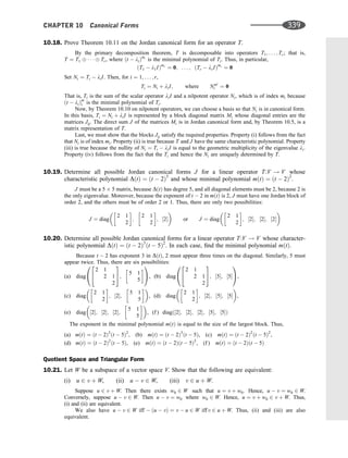
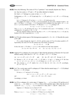
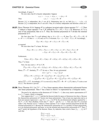
![Now let v2; . . . ; vn be elements of V that belong to the cosets v2; . . . ; vn, respectively. Then fv; v2; . . . ; vng
is a basis of V (Problem 10.26). Because
Tðv2Þ ¼ a22
v2, we have
Tð
v2Þ a22
v22 ¼ 0; and so Tðv2Þ a22v2 2 W
But W is spanned by v; hence, Tðv2Þ a22v2 is a multiple of v, say,
Tðv2Þ a22v2 ¼ a21v; and so Tðv2Þ ¼ a21v þ a22v2
Similarly, for i ¼ 3; . . . ; n
TðviÞ ai2v2 ai3v3 aiivi 2 W; and so TðviÞ ¼ ai1v þ ai2v2 þ þ aiivi
Thus,
TðvÞ ¼ a11v
Tðv2Þ ¼ a21v þ a22v2
::::::::::::::::::::::::::::::::::::::::
TðvnÞ ¼ an1v þ an2v2 þ þ annvn
and hence the matrix of T in this basis is triangular.
Cyclic Subspaces, Rational Canonical Form
10.29. Prove Theorem 10.12: Let Zðv; TÞ be a T-cyclic subspace, Tv the restriction of T to Zðv; TÞ, and
mvðtÞ ¼ tk
þ ak1tk1
þ þ a0 the T-annihilator of v. Then,
(i) The set fv; TðvÞ; . . . ; Tk1
ðvÞg is a basis of Zðv; TÞ; hence, dim Zðv; TÞ ¼ k.
(ii) The minimal polynomial of Tv is mvðtÞ.
(iii) The matrix of Tv in the above basis is the companion matrix C ¼ CðmvÞ of mvðtÞ [which
has 1’s below the diagonal, the negative of the coefficients a0; a1; . . . ; ak1 of mvðtÞ in the
last column, and 0’s elsewhere].
(i) By definition of mvðtÞ, Tk
ðvÞ is the first vector in the sequence v, TðvÞ, T2
ðvÞ; ... that, is a linear
combination of those vectors that precede it in the sequence; hence, the set B ¼ fv; TðvÞ; ... ; Tk1
ðvÞg is
linearly independent. We now only have to show that Zðv; TÞ ¼ LðBÞ, the linear span of B. By the above,
Tk
ðvÞ 2 LðBÞ. We prove by induction that Tn
ðvÞ 2 LðBÞ for every n. Suppose n k and
Tn1
ðvÞ 2 LðBÞ—that is, Tn1
ðvÞ is a linear combination of v; ... ; Tk1
ðvÞ. Then
Tn
ðvÞ ¼ TðTn1
ðvÞÞ is a linear combination of TðvÞ; ... ; Tk
ðvÞ. But Tk
ðvÞ 2 LðBÞ; hence,
Tn
ðvÞ 2 LðBÞ for every n. Consequently, f ðTÞðvÞ 2 LðBÞ for any polynomial f ðtÞ. Thus,
Zðv; TÞ ¼ LðBÞ, and so B is a basis, as claimed.
(ii) Suppose mðtÞ ¼ ts
þ bs1ts1
þ þ b0 is the minimal polynomial of Tv. Then, because v 2 Zðv; TÞ,
0 ¼ mðTvÞðvÞ ¼ mðTÞðvÞ ¼ Ts
ðvÞ þ bs1Ts1
ðvÞ þ þ b0v
Thus, Ts
ðvÞ is a linear combination of v, TðvÞ; . . . ; Ts1
ðvÞ, and therefore k s. However,
mvðTÞ ¼ 0 and so mvðTvÞ ¼ 0: Then mðtÞ divides mvðtÞ; and so s k: Accordingly, k ¼ s and
hence mvðtÞ ¼ mðtÞ.
(iii)
TvðvÞ ¼ TðvÞ
TvðTðvÞÞ ¼ T2
ðvÞ
:::::::::::::::::::::::::::::::::::::::::::::::::::::::::::::::::::::::::::::::::::::::::::::::::::::::::
TvðTk2
ðvÞÞ ¼ Tk1
ðvÞ
TvðTk1
ðvÞÞ ¼ Tk
ðvÞ ¼ a0v a1 TðvÞ a2T2
ðvÞ ak1 Tk1
ðvÞ
By definition, the matrix of Tv in this basis is the tranpose of the matrix of coefficients of the above
system of equations; hence, it is C, as required.
10.30. Let T:V ! V be linear. Let W be a T-invariant subspace of V and
T the induced operator on
V=W. Prove
(a) The T-annihilator of v 2 V divides the minimal polynomial of T.
(b) The
T-annihilator of
v 2 V=W divides the minimal polynomial of T.
342 CHAPTER 10 Canonical Forms](https://image.slidesharecdn.com/linearalgebra4thedition-231030053714-df1faee2/85/Linear_Algebra-_4th_Edition-pdf-349-320.jpg)
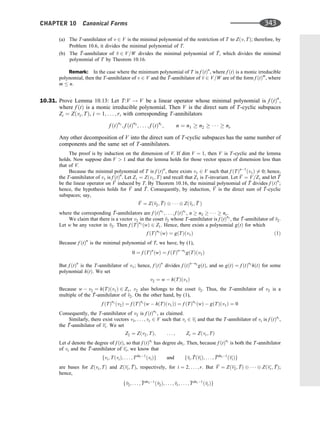
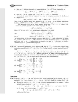
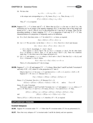
![10.38. Let W be invariant under T1: V ! V and T2: V ! V. Prove W is also invariant under T1 þ T2 and T1T2.
10.39. Let T:V ! V be linear. Prove that any eigenspace, El is T-invariant.
10.40. Let V be a vector space of odd dimension (greater than 1) over the real field R. Show that any linear
operator on V has an invariant subspace other than V or f0g.
10.41. Determine the invariant subspace of A ¼
2 4
5 2
viewed as a linear operator on (a) R2
, (b) C2
.
10.42. Suppose dim V ¼ n. Show that T:V ! V has a triangular matrix representation if and only if there exist
T-invariant subspaces W1 W2 Wn ¼ V for which dim Wk ¼ k, k ¼ 1; . . . ; n.
Invariant Direct Sums
10.43. The subspaces W1; . . . ; Wr are said to be independent if w1 þ þ wr ¼ 0, wi 2 Wi, implies that each
wi ¼ 0. Show that spanðWiÞ ¼ W1 Wr if and only if the Wi are independent. [Here spanðWiÞ
denotes the linear span of the Wi.]
10.44. Show that V ¼ W1 Wr if and only if (i) V ¼ spanðWiÞ and (ii) for k ¼ 1; 2; . . . ; r,
Wk spanðW1; . . . ; Wk1; Wkþ1; . . . ; WrÞ ¼ f0g.
10.45. Show that spanðWiÞ ¼ W1 Wr if and only if dim ½spanðWiÞ ¼ dim W1 þ þ dim Wr.
10.46. Suppose the characteristic polynomial of T:V ! V is DðtÞ ¼ f1ðtÞn1
f2ðtÞn2
frðtÞnr
, where the fiðtÞ are
distinct monic irreducible polynomials. Let V ¼ W1 Wr be the primary decomposition of V into T-
invariant subspaces. Show that fiðtÞni
is the characteristic polynomial of the restriction of T to Wi.
Nilpotent Operators
10.47. Suppose T1 and T2 are nilpotent operators that commute (i.e., T1T2 ¼ T2T1). Show that T1 þ T2 and T1T2
are also nilpotent.
10.48. Suppose A is a supertriangular matrix (i.e., all entries on and below the main diagonal are 0). Show that A is
nilpotent.
10.49. Let V be the vector space of polynomials of degree n. Show that the derivative operator on V is nilpotent
of index n þ 1.
10.50. Show that any Jordan nilpotent block matrix N is similar to its transpose NT
(the matrix with 1’s below the
diagonal and 0’s elsewhere).
10.51. Show that two nilpotent matrices of order 3 are similar if and only if they have the same index of
nilpotency. Show by example that the statement is not true for nilpotent matrices of order 4.
Jordan Canonical Form
10.52. Find all possible Jordan canonical forms for those matrices whose characteristic polynomial DðtÞ and
minimal polynomial mðtÞ are as follows:
(a) DðtÞ ¼ ðt 2Þ4
ðt 3Þ2
; mðtÞ ¼ ðt 2Þ2
ðt 3Þ2
,
(b) DðtÞ ¼ ðt 7Þ5
; mðtÞ ¼ ðt 7Þ2
, (c) DðtÞ ¼ ðt 2Þ7
; mðtÞ ¼ ðt 2Þ3
10.53. Show that every complex matrix is similar to its transpose. (Hint: Use its Jordan canonical form.)
10.54. Show that all n n complex matrices A for which An
¼ I but Ak 6¼ I for k n are similar.
10.55. Suppose A is a complex matrix with only real eigenvalues. Show that A is similar to a matrix with only real
entries.
346 CHAPTER 10 Canonical Forms](https://image.slidesharecdn.com/linearalgebra4thedition-231030053714-df1faee2/85/Linear_Algebra-_4th_Edition-pdf-353-320.jpg)
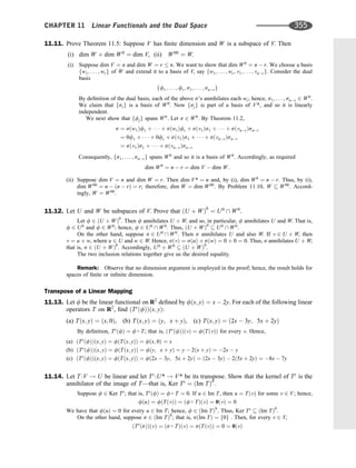
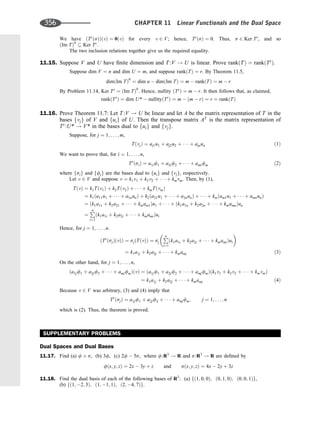
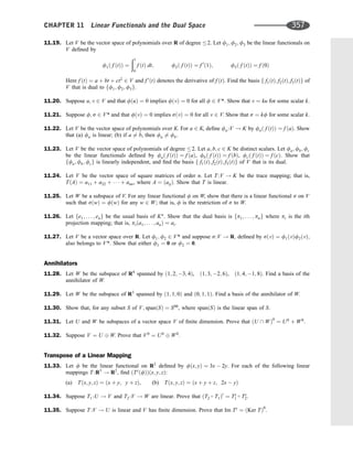
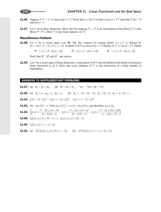
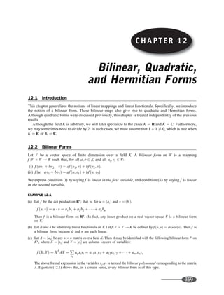
![Space of Bilinear Forms
Let BðVÞ denote the set of all bilinear forms on V. A vector space structure is placed on BðVÞ, where for
any f ; g 2 BðVÞ and any k 2 K, we define f þ g and kf as follows:
ð f þ gÞðu; vÞ ¼ f ðu; vÞ þ gðu; vÞ and ðkf Þðu; vÞ ¼ kf ðu; vÞ
The following theorem (proved in Problem 12.4) applies.
THEOREM 12.1: Let V be a vector space of dimension n over K. Let ff1; . . . ; fng be any basis of the
dual space V*. Then f fij : i; j ¼ 1; . . . ; ng is a basis of BðVÞ, where fij is defined by
fijðu; vÞ ¼ fiðuÞfjðvÞ. Thus, in particular, dim BðVÞ ¼ n2
.
12.3 Bilinear Forms and Matrices
Let f be a bilinear form on V and let S ¼ fu1; . . . ; ung be a basis of V. Suppose u; v 2 V and
u ¼ a1u1 þ þ anun and v ¼ b1u1 þ þ bnun
Then
f ðu; vÞ ¼ f ða1u1 þ þ anun; b1u1 þ þ bnunÞ ¼
P
i;j
aibjf ðui; ujÞ
Thus, f is completely determined by the n2
values f ðui; ujÞ.
The matrix A ¼ ½aij where aij ¼ f ðui; ujÞ is called the matrix representation of f relative to the basis S
or, simply, the ‘‘matrix of f in S.’’ It ‘‘represents’’ f in the sense that, for all u; v 2 V,
f ðu; vÞ ¼
P
i;j
aibj f ðui; ujÞ ¼ ½uT
S A½vS ð12:1Þ
[As usual, ½uS denotes the coordinate (column) vector of u in the basis S.]
Change of Basis, Congruent Matrices
We now ask, how does a matrix representing a bilinear form transform when a new basis is selected? The
answer is given in the following theorem (proved in Problem 12.5).
THEOREM 12.2: Let P be a change-of-basis matrix from one basis S to another basis S0
. If A is the
matrix representing a bilinear form f in the original basis S, then B ¼ PT
AP is the
matrix representing f in the new basis S0
.
The above theorem motivates the following definition.
DEFINITION: A matrix B is congruent to a matrix A, written B ’ A, if there exists a nonsingular
matrix P such that B ¼ PT
AP.
Thus, by Theorem 12.2, matrices representing the same bilinear form are congruent. We remark that
congruent matrices have the same rank, because P and PT
are nonsingular; hence, the following definition
is well defined.
DEFINITION: The rank of a bilinear form f on V, written rankð f Þ, is the rank of any matrix
representation of f . We say f is degenerate or nondegenerate according to whether
rankð f Þ dim V or rankð f Þ ¼ dim V.
12.4 Alternating Bilinear Forms
Let f be a bilinear form on V. Then f is called
(i) alternating if f ðv; vÞ ¼ 0 for every v 2 V;
(ii) skew-symmetric if f ðu; vÞ ¼ f ðv; uÞ for every u; v 2 V.
360 CHAPTER 12 Bilinear, Quadratic, and Hermitian Forms](https://image.slidesharecdn.com/linearalgebra4thedition-231030053714-df1faee2/85/Linear_Algebra-_4th_Edition-pdf-367-320.jpg)
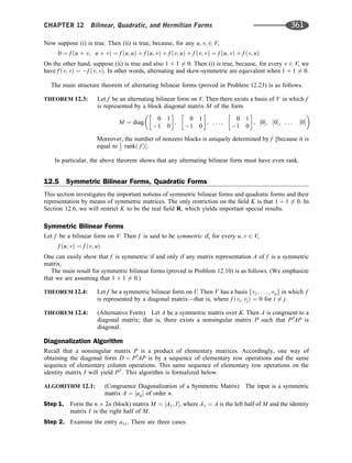
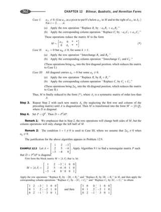
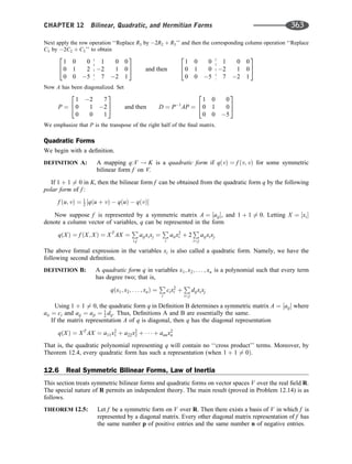
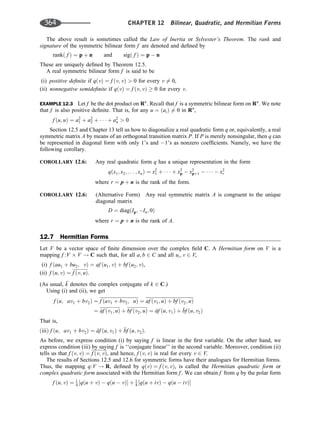
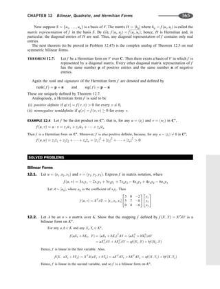
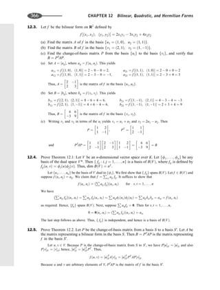
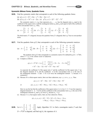
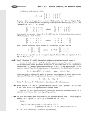
![12.12. Consider the quadratic form qðx; yÞ ¼ 3x2
þ 2xy y2
and the linear substitution
x ¼ s 3t; y ¼ 2s þ t
(a) Rewrite qðx; yÞ in matrix notation, and find the matrix A representing qðx; yÞ.
(b) Rewrite the linear substitution using matrix notation, and find the matrix P corresponding to
the substitution.
(c) Find qðs; tÞ using direct substitution.
(d) Find qðs; tÞ using matrix notation.
(a) Here qðx; yÞ ¼ ½x; y
3 1
1 1
x
y
. Thus, A ¼
3 1
1 1
; and qðXÞ ¼ XT
AX, where X ¼ ½x; yT
.
(b) Here
x
y
¼
1 3
2 1
s
t
. Thus, P ¼
1 3
2 1
; and X ¼
x
y
; Y ¼
s
t
and X ¼ PY.
(c) Substitute for x and y in q to obtain
qðs; tÞ ¼ 3ðs 3tÞ2
þ 2ðs 3tÞð2s þ tÞ ð2s þ tÞ2
¼ 3ðs2
6st þ 9t2
Þ þ 2ð2s2
5st 3t2
Þ ð4s2
þ 4st þ t2
Þ ¼ 3s2
32st þ 20t2
(d) Here qðXÞ ¼ XT
AX and X ¼ PY. Thus, XT
¼ YT
PT
. Therefore,
qðs; tÞ ¼ qðYÞ ¼ YT
PT
APY ¼ ½s; t
1 2
3 1
3 1
1 1
1 3
2 1
s
t
¼ ½s; t
3 16
16 20
s
t
¼ 3s2
32st þ 20t2
[As expected, the results in parts (c) and (d) are equal.]
12.13. Consider any diagonal matrix A ¼ diagða1; . . . ; anÞ over K. Show that for any nonzero scalars
k1; . . . ; kn 2 K; A is congruent to a diagonal matrix D with diagonal entries a1k2
1; . . . ; ank2
n.
Furthermore, show that
(a) If K ¼ C, then we can choose D so that its diagonal entries are only 1’s and 0’s.
(b) If K ¼ R, then we can choose D so that its diagonal entries are only 1’s, 1’s, and 0’s.
Let P ¼ diagðk1; . . . ; knÞ. Then, as required,
D ¼ PT
AP ¼ diagðkiÞ diagðaiÞ diagðkiÞ ¼ diagða1k2
1 ; . . . ; ank2
n Þ
(a) Let P ¼ diagðbiÞ, where bi ¼
1=
ffiffiffiffi
ai
p
if ai 6¼ 0
1 if ai ¼ 0
Then PT
AP has the required form.
(b) Let P ¼ diagðbiÞ, where bi ¼
1=
ffiffiffiffiffiffiffi
jaij
p
if ai 6¼ 0
1 if ai ¼ 0
Then PT
AP has the required form.
Remark: We emphasize that (b) is no longer true if ‘‘congruence’’ is replaced by
‘‘Hermitian congruence.’’
12.14. Prove Theorem 12.5: Let f be a symmetric bilinear form on V over R. Then there exists a basis
of V in which f is represented by a diagonal matrix. Every other diagonal matrix representation
of f has the same number p of positive entries and the same number n of negative entries.
By Theorem 12.4, there is a basis fu1; . . . ; ung of V in which f is represented by a diagonal matrix
with, say, p positive and n negative entries. Now suppose fw1; . . . ; wng is another basis of V, in which f is
represented by a diagonal matrix with p0
positive and n0
negative entries. We can assume without loss of
generality that the positive entries in each matrix appear first. Because rankð f Þ ¼ p þ n ¼ p0
þ n0
, it
suffices to prove that p ¼ p0
.
CHAPTER 12 Bilinear, Quadratic, and Hermitian Forms 369](https://image.slidesharecdn.com/linearalgebra4thedition-231030053714-df1faee2/85/Linear_Algebra-_4th_Edition-pdf-376-320.jpg)
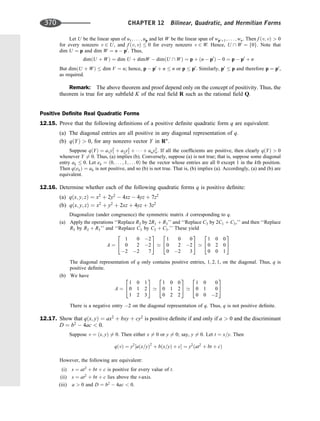
![Thus, q is positive definite if and only if a 0 and D 0. [Remark: D 0 is the same as detðAÞ 0,
where A is the symmetric matrix corresponding to q.]
12.18. Determine whether or not each of the following quadratic forms q is positive definite:
(a) qðx; yÞ ¼ x2
4xy þ 7y2
, (b) qðx; yÞ ¼ x2
þ 8xy þ 5y2
, (c) qðx; yÞ ¼ 3x2
þ 2xy þ y2
Compute the discriminant D ¼ b2
4ac, and then use Problem 12.17.
(a) D ¼ 16 28 ¼ 12. Because a ¼ 1 0 and D 0; q is positive definite.
(b) D ¼ 64 20 ¼ 44. Because D 0; q is not positive definite.
(c) D ¼ 4 12 ¼ 8. Because a ¼ 3 0 and D 0; q is positive definite.
Hermitian Forms
12.19. Determine whether the following matrices are Hermitian:
(a)
2 2 þ 3i 4 5i
2 3i 5 6 þ 2i
4 þ 5i 6 2i 7
2
4
3
5, (b)
3 2 i 4 þ i
2 i 6 i
4 þ i i 7
2
4
3
5, (c)
4 3 5
3 2 1
5 1 6
2
4
3
5
A complex matrix A ¼ ½aij is Hermitian if A* ¼ A—that is, if aij ¼
aji:
(a) Yes, because it is equal to its conjugate transpose.
(b) No, even though it is symmetric.
(c) Yes. In fact, a real matrix is Hermitian if and only if it is symmetric.
12.20. Let A be a Hermitian matrix. Show that f is a Hermitian form on Cn
where f is defined by
f ðX; YÞ ¼ XT
A
Y.
For all a; b 2 C and all X1; X2; Y 2 Cn
,
f ðaX1 þ bX2; YÞ ¼ ðaX1 þ bX2ÞT
A
Y ¼ ðaXT
1 þ bXT
2 ÞA
Y
¼ aXT
1 A
Y þ bXT
2 A
Y ¼ af ðX1; YÞ þ bf ðX2; YÞ
Hence, f is linear in the first variable. Also,
f ðX; YÞ ¼ XTA
Y ¼ ðXTA
YÞT
¼
YT AT X ¼ YT
A*
X ¼ YT
A
X ¼ f ðY; XÞ
Hence, f is a Hermitian form on Cn
.
Remark: We use the fact that XT
A
Y is a scalar and so it is equal to its transpose.
12.21. Let f be a Hermitian form on V. Let H be the matrix of f in a basis S ¼ fuig of V. Prove the
following:
(a) f ðu; vÞ ¼ ½uT
S H½vS for all u; v 2 V.
(b) If P is the change-of-basis matrix from S to a new basis S0
of V, then B ¼ PT
H
P (or
B ¼ Q*HQ, where Q ¼
PÞ is the matrix of f in the new basis S0
.
Note that (b) is the complex analog of Theorem 12.2.
(a) Let u; v 2 V and suppose u ¼ a1u1 þ þ anun and v ¼ b1u1 þ þ bnun. Then, as required,
f ðu; vÞ ¼ f ða1u1 þ þ anun; b1u1 þ þ bnunÞ
¼
P
i;j
ai
bjf ðui; vjÞ ¼ ½a1; . . . ; anH½
b1; . . . ;
bnT
¼ ½uT
S H½vS
CHAPTER 12 Bilinear, Quadratic, and Hermitian Forms 371](https://image.slidesharecdn.com/linearalgebra4thedition-231030053714-df1faee2/85/Linear_Algebra-_4th_Edition-pdf-378-320.jpg)
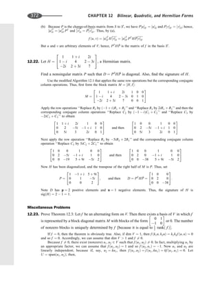
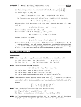
![(a) The set BðV; WÞ of bilinear forms on V and W is a subspace of the vector space of functions from
V W into K.
(b) If ff1; ... ; fmg is a basis of V* and fs1; ... ; sng is a basis of W*, then
f fij : i ¼ 1; ... ; m; j ¼ 1; ... ; ng is a basis of BðV; WÞ, where fij is defined by fijðv; wÞ ¼ fiðvÞsjðwÞ.
Thus, dim BðV; WÞ ¼ dim V dim W.
[Note that if V ¼ W, then we obtain the space BðVÞ investigated in this chapter.]
12.50. Let V be a vector space over K. A mapping f :V V . . . V
zfflfflfflfflfflfflfflfflfflfflfflfflffl}|fflfflfflfflfflfflfflfflfflfflfflfflffl{
m times
! K is called a multilinear (or m-linear)
form on V if f is linear in each variable; that is, for i ¼ 1; . . . ; m,
f ð. . . ; au þ bv; . . .Þ ¼ af ð. . . ; ^
u; . . .Þ þ bf ð. . . ; ^
v; . . .Þ
where c
. . . denotes the ith element, and other elements are held fixed. An m-linear form f is said to be
alternating if f ðv1; . . . vmÞ ¼ 0 whenever vi ¼ vj for i 6¼ j. Prove the following:
(a) The set BmðVÞ of m-linear forms on V is a subspace of the vector space of functions from
V V V into K.
(b) The set AmðVÞ of alternating m-linear forms on V is a subspace of BmðVÞ.
Remark 1: If m ¼ 2, then we obtain the space BðVÞ investigated in this chapter.
Remark 2: If V ¼ Km
, then the determinant function is an alternating m-linear form on V.
ANSWERS TO SUPPLEMENTARY PROBLEMS
Notation: M ¼ ½R1; R2; . . . denotes a matrix M with rows R1; R2; . . ..
12.24. (a) yes, (b) no, (c) yes, (d) no, (e) no, (f ) yes
12.25. (a) A ¼ ½4; 1; 7; 3, (b) B ¼ ½0; 4; 20; 32, (c) P ¼ ½3; 5; 2; 2
12.26. (b) ½1; 0; 2; 0; 0; 1; 0; 2; 3; 0; 5; 0; 0; 3; 0; 5
12.33. (a) ½2; 4; 8; 4; 1; 7; 8; 7; 5, (b) ½1; 0; 1
2 ; 0; 1; 0; 1
2 ; 0; 0,
(c) ½0; 1
2 ; 2; 1
2 ; 1; 0; 2; 0; 1, (d) ½0; 1
2 ; 0; 1
2 ; 0; 1; 1
2 ; 0; 1
2 ; 0; 1
2 ; 0
12.34. (a) P ¼ ½1; 0; 2; 0; 1; 2; 0; 0; 1; D ¼ diagð1; 3; 9Þ;
(b) P ¼ ½1; 2; 11; 0; 1; 5; 0; 0; 1; D ¼ diagð1; 1; 28Þ;
(c) P ¼ ½1; 1; 1; 4; 0; 1; 1; 2; 0; 0; 1; 0; 0; 0; 0; 1; D ¼ diagð1; 1; 0; 9Þ
12.35. A ¼ ½2; 3; 3; 3, P ¼ ½1; 2; 3; 1, qðs; tÞ ¼ 43s2
4st þ 17t2
12.36. (a) x ¼ r 3s 19t, y ¼ s þ 7t, z ¼ t; qðr; s; tÞ ¼ r2
s2
þ 36t2
;
(b) x ¼ r 2t; y ¼ s þ 2t; z ¼ t; qðr; s; tÞ ¼ 2r2
3s2
þ 29t2
;
(c) x ¼ r s t; y ¼ s t; z ¼ t; qðr; s; tÞ ¼ r2
2s2
12.37. qðx; yÞ ¼ x2
y2
, u ¼ ð1; 1Þ, v ¼ ð1; 1Þ
12.40. (a) yes, (b) no, (c) no, (d) yes
12.41. (a) k 25
8 , (b) 12 k 12, (c) k 5
12.44. (a) P ¼ ½1; i; 0; 1, D ¼ I; s ¼ 2; (b) P ¼ ½1; 2 þ 3i; 0; 1, D ¼ diagð1; 14Þ, s ¼ 0;
(c) P ¼ ½1; i; 3 þ i; 0; 1; i; 0; 0; 1, D ¼ diagð1; 1; 4Þ; s ¼ 1
d
376 CHAPTER 12 Bilinear, Quadratic, and Hermitian Forms](https://image.slidesharecdn.com/linearalgebra4thedition-231030053714-df1faee2/85/Linear_Algebra-_4th_Edition-pdf-383-320.jpg)
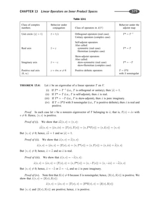
![Remark: Each of the above operators T commutes with its adjoint; that is, TT* ¼ T*T. Such
operators are called normal operators.
13.4 Self-Adjoint Operators
Let T be a self-adjoint operator on an inner product space V; that is, suppose
T* ¼ T
(If T is defined by a matrix A, then A is symmetric or Hermitian according as A is real or complex.) By
Theorem 13.4, the eigenvalues of T are real. The following is another important property of T.
THEOREM 13.5: Let T be a self-adjoint operator on V. Suppose u and v are eigenvectors of T
belonging to distinct eigenvalues. Then u and v are orthogonal; that is, hu; vi ¼ 0.
Proof. Suppose TðuÞ ¼ l1u and TðvÞ ¼ l2v, where l1 6¼ l2. We show that l1hu; vi ¼ l2hu; vi:
l1hu; vi ¼ hl1u; vi ¼ hTðuÞ; vi ¼ hu; T*ðvÞi ¼ hu; TðvÞi
¼ hu; l2vi ¼
l2hu; vi ¼ l2hu; vi
(The fourth equality uses the fact that T* ¼ T, and the last equality uses the fact that the eigenvalue l2 is
real.) Because l1 6¼ l2, we get hu; vi ¼ 0. Thus, the theorem is proved.
13.5 Orthogonal and Unitary Operators
Let U be a linear operator on a finite-dimensional inner product space V. Suppose
U* ¼ U1
or equivalently UU* ¼ U*U ¼ I
Recall that U is said to be orthogonal or unitary according as the underlying field is real or complex. The
next theorem (proved in Problem 13.10) gives alternative characterizations of these operators.
THEOREM 13.6: The following conditions on an operator U are equivalent:
(i) U* ¼ U1
; that is, UU* ¼ U*U ¼ I. [U is unitary (orthogonal).]
(ii) U preserves inner products; that is, for every v; w 2 V,
hUðvÞ, UðwÞi ¼ hv; wi.
(iii) U preserves lengths; that is, for every v 2 V, kUðvÞk ¼ kvk.
EXAMPLE 13.2
(a) Let T :R3
! R3
be the linear operator that rotates each vector v about the z-axis by a fixed angle y as shown in
Fig. 10-1 (Section 10.3). That is, T is defined by
Tðx; y; zÞ ¼ ðx cos y y sin y; x sin y þ y cos y; zÞ
We note that lengths (distances from the origin) are preserved under T. Thus, T is an orthogonal operator.
(b) Let V be l2-space (Hilbert space), defined in Section 7.3. Let T :V ! V be the linear operator defined by
Tða1; a2; a3; . . .Þ ¼ ð0; a1; a2; a3; . . .Þ
Clearly, T preserves inner products and lengths. However, T is not surjective, because, for example, ð1; 0; 0; . . .Þ
does not belong to the image of T; hence, T is not invertible. Thus, we see that Theorem 13.6 is not valid for
spaces of infinite dimension.
An isomorphism from one inner product space into another is a bijective mapping that preserves the
three basic operations of an inner product space: vector addition, scalar multiplication, and inner
380 CHAPTER 13 Linear Operators on Inner Product Spaces](https://image.slidesharecdn.com/linearalgebra4thedition-231030053714-df1faee2/85/Linear_Algebra-_4th_Edition-pdf-387-320.jpg)
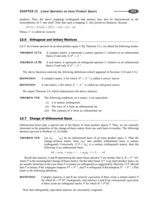
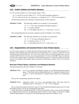
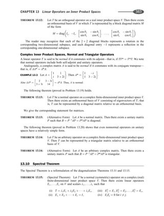
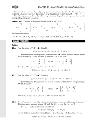
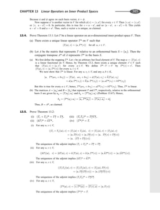
![13.6. Show that ðaÞ I* ¼ I, and ðbÞ 0* ¼ 0.
(a) For every u; v 2 V, hIðuÞ; vi ¼ hu; vi ¼ hu; IðvÞi; hence, I* ¼ I.
(b) For every u; v 2 V, h0ðuÞ; vi ¼ h0; vi ¼ 0 ¼ hu; 0i ¼ hu; 0ðvÞi; hence, 0* ¼ 0.
13.7. Suppose T is invertible. Show that ðT1
Þ* ¼ ðT*Þ1
.
I ¼ I* ¼ ðTT1
Þ* ¼ ðT1
Þ*T*; hence; ðT1
Þ* ¼ ðT*Þ1
:
13.8. Let T be a linear operator on V, and let W be a T-invariant subspace of V. Show that W?
is
invariant under T*.
Let u 2 W?
. If w 2 W, then TðwÞ 2 W and so hw; T*ðuÞi ¼ hTðwÞ; ui ¼ 0. Thus, T*ðuÞ 2 W?
because it is orthogonal to every w 2 W. Hence, W?
is invariant under T*.
13.9. Let T be a linear operator on V. Show that each of the following conditions implies T ¼ 0:
(i) hTðuÞ; vi ¼ 0 for every u; v 2 V.
(ii) V is a complex space, and hTðuÞ; ui ¼ 0 for every u 2 V.
(iii) T is self-adjoint and hTðuÞ; ui ¼ 0 for every u 2 V.
Give an example of an operator T on a real space V for which hTðuÞ; ui ¼ 0 for every u 2 V but T 6¼ 0.
[Thus, (ii) need not hold for a real space V.]
(i) Set v ¼ TðuÞ. Then hTðuÞ; TðuÞi ¼ 0, and hence, TðuÞ ¼ 0, for every u 2 V. Accordingly, T ¼ 0.
(ii) By hypothesis, hTðv þ wÞ; v þ wi ¼ 0 for any v; w 2 V. Expanding and setting hTðvÞ; vi ¼ 0 and
hTðwÞ; wi ¼ 0, we find
hTðvÞ; wi þ hTðwÞ; vi ¼ 0 ð1Þ
Note w is arbitrary in (1). Substituting iw for w, and using hTðvÞ; iwi ¼
ihTðvÞ; wi ¼ ihTðvÞ; wi and
hTðiwÞ; vi ¼ hiTðwÞ; vi ¼ ihTðwÞ; vi, we find
ihTðvÞ; wi þ ihTðwÞ; vi ¼ 0
Dividing through by i and adding to (1), we obtain hTðwÞ; vi ¼ 0 for any v; w; 2 V. By (i), T ¼ 0.
(iii) By (ii), the result holds for the complex case; hence we need only consider the real case. Expanding
hTðv þ wÞ; v þ wi ¼ 0, we again obtain (1). Because T is self-adjoint and as it is a real space, we
have hTðwÞ; vi ¼ hw; TðvÞi ¼ hTðvÞ; wi. Substituting this into (1), we obtain hTðvÞ; wi ¼ 0 for any
v; w 2 V. By (i), T ¼ 0.
For an example, consider the linear operator T on R2
defined by Tðx; yÞ ¼ ðy; xÞ. Then
hTðuÞ; ui ¼ 0 for every u 2 V, but T 6¼ 0.
Orthogonal and Unitary Operators and Matrices
13.10. Prove Theorem 13.6: The following conditions on an operator U are equivalent:
(i) U* ¼ U1
; that is, U is unitary. (ii) hUðvÞ; UðwÞi ¼ hu; wi. (iii) kUðvÞk ¼ kvk.
Suppose (i) holds. Then, for every v; w; 2 V,
hUðvÞ; UðwÞi ¼ hv; U*UðwÞi ¼ hv; IðwÞi ¼ hv; wi
Thus, (i) implies (ii). Now if (ii) holds, then
kUðvÞk ¼
ffiffiffiffiffiffiffiffiffiffiffiffiffiffiffiffiffiffiffiffiffiffiffiffiffiffi
hUðvÞ; UðvÞi
p
¼
ffiffiffiffiffiffiffiffiffiffiffi
hv; vi
p
¼ kvk
Hence, (ii) implies (iii). It remains to show that (iii) implies (i).
Suppose (iii) holds. Then for every v 2 V,
hU*UðvÞi ¼ hUðvÞ; UðvÞi ¼ hv; vi ¼ hIðvÞ; vi
Hence, hðU*U IÞðvÞ; vi ¼ 0 for every v 2 V. But U*U I is self-adjoint (Prove!); then, by Problem
13.9, we have U*U I ¼ 0 and so U*U ¼ I. Thus, U* ¼ U1
, as claimed.
386 CHAPTER 13 Linear Operators on Inner Product Spaces](https://image.slidesharecdn.com/linearalgebra4thedition-231030053714-df1faee2/85/Linear_Algebra-_4th_Edition-pdf-393-320.jpg)
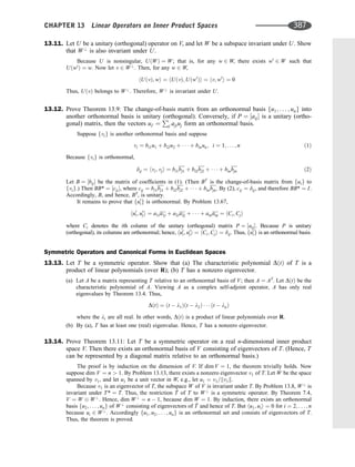
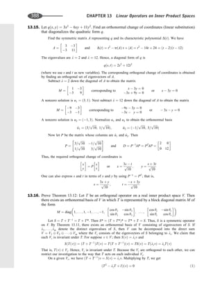
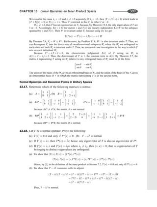
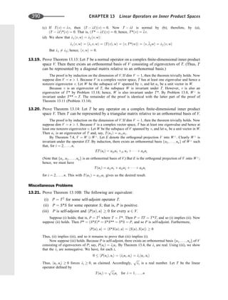
![Because T is represented by a real diagonal matrix relative to the orthonormal basis fuig, T is self-adjoint.
Moreover, for each i,
T2
ðuiÞ ¼ Tð
ffiffiffiffi
li
p
uiÞ ¼
ffiffiffiffi
li
p
TðiiÞ ¼
ffiffiffiffi
li
p ffiffiffiffi
li
p
ui ¼ liui ¼ PðuiÞ
Because T2
and P agree on a basis of V; P ¼ T2
. Thus, the theorem is proved.
Remark: The above operator T is the unique positive operator such that P ¼ T2
; it is called the
positive square root of P.
13.22. Show that any operator T is the sum of a self-adjoint operator and a skew-adjoint operator.
Set S ¼ 1
2 ðT þ T*Þ and U ¼ 1
2 ðT T*Þ: Then T ¼ S þ U; where
S* ¼ ½1
2 ðT þ T*Þ* ¼ 1
2 ðT* þ T**Þ ¼ 1
2 ðT* þ TÞ ¼ S
U* ¼ ½1
2 ðT T*Þ* ¼ 1
2 ðT* TÞ ¼ 1
2 ðT T*Þ ¼ U
and
that is, S is self-adjoint and U is skew-adjoint.
13.23. Prove: Let T be an arbitrary linear operator on a finite-dimensional inner product space V. Then
T is a product of a unitary (orthogonal) operator U and a unique positive operator P; that is,
T ¼ UP. Furthermore, if T is invertible, then U is also uniquely determined.
By Theorem 13.10, T*T is a positive operator; hence, there exists a (unique) positive operator P such
that P2
¼ T*T (Problem 13.43). Observe that
kPðvÞk2
¼ hPðvÞ; PðvÞi ¼ hP2
ðvÞ; vi ¼ hT*TðvÞ; vi ¼ hTðvÞ; TðvÞi ¼ kTðvÞk2
ð1Þ
We now consider separately the cases when T is invertible and noninvertible.
If T is invertible, then we set ^
U ¼ PT1
. We show that ^
U is unitary:
^
U* ¼ ðPT1
Þ* ¼ T1
P* ¼ ðT*Þ1
P and ^
U ^
U ¼ ðT*Þ1
PPT1
¼ ðT*Þ1
T*TT1
¼ I
Thus, ^
U is unitary. We next set U ¼ ^
U1
. Then U is also unitary, and T ¼ UP as required.
To prove uniqueness, we assume T ¼ U0P0, where U0 is unitary and P0 is positive. Then
T*T ¼ P0
*U0
*U0P0 ¼ P0IP0 ¼ P2
0
But the positive square root of T*T is unique (Problem 13.43); hence, P0 ¼ P. (Note that the invertibility
of T is not used to prove the uniqueness of P.) Now if T is invertible, then P is also invertible by (1).
Multiplying U0P ¼ UP on the right by P1
yields U0 ¼ U. Thus, U is also unique when T is invertible.
Now suppose T is not invertible. Let W be the image of P; that is, W ¼ Im P. We define U1 :W ! V by
U1ðwÞ ¼ TðvÞ; where PðvÞ ¼ w ð2Þ
We must show that U1 is well defined; that is, that PðvÞ ¼ Pðv0
Þ implies TðvÞ ¼ Tðv0
Þ. This follows from
the fact that Pðv v0
Þ ¼ 0 is equivalent to kPðv v0
Þk ¼ 0, which forces kTðv v0
Þk ¼ 0 by (1). Thus,
U1 is well defined. We next define U2 :W ! V. Note that, by (1), P and T have the same kernels. Hence, the
images of P and T have the same dimension; that is, dimðIm PÞ ¼ dim W ¼ dimðIm TÞ. Consequently,
W?
and ðIm TÞ?
also have the same dimension. We let U2 be any isomorphism between W?
and ðIm TÞ?
.
We next set U ¼ U1 U2. [Here U is defined as follows: If v 2 V and v ¼ w þ w0
, where w 2 W,
w0
2 W?
, then UðvÞ ¼ U1ðwÞ þ U2ðw0
Þ.] Now U is linear (Problem 13.69), and, if v 2 V and PðvÞ ¼ w,
then, by (2),
TðvÞ ¼ U1ðwÞ ¼ UðwÞ ¼ UPðvÞ
Thus, T ¼ UP, as required.
It remains to show that U is unitary. Now every vector x 2 V can be written in the form x ¼ PðvÞ þ w0
,
where w0
2 W?
. Then UðxÞ ¼ UPðvÞ þ U2ðw0
Þ ¼ TðvÞ þ U2ðw0
Þ, where hTðvÞ; U2ðw0
Þi ¼ 0 by definition
CHAPTER 13 Linear Operators on Inner Product Spaces 391](https://image.slidesharecdn.com/linearalgebra4thedition-231030053714-df1faee2/85/Linear_Algebra-_4th_Edition-pdf-398-320.jpg)
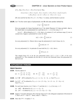
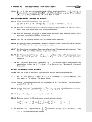
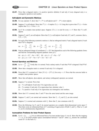
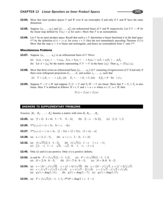
![Multilinear Products
A.1 Introduction
The material in this appendix is much more abstract than that which has previously appeared. Accordingly,
many of the proofs will be omitted. Also, we motivate the material with the following observation.
Let S be a basis of a vector space V. Theorem 5.2 may be restated as follows.
THEOREM 5.2: Let g:S ! V be the inclusion map of the basis S into V. Then, for any vector space
U and any mapping f :S ! U; there exists a unique linear mapping f
:V ! U such
that f ¼ f
g:
Another way to state the fact that f ¼ f
g is that the diagram in Fig. A-1(a) commutes.
A.2 Bilinear Mapping and Tensor Products
Let U, V, W be vector spaces over a field K. Consider a map
f : V W ! U
Then f is said to be bilinear if, for each v 2 V; the map fv :W ! U defined by fv w
ð Þ ¼ f v; w
ð Þ is linear;
and, for each w 2 W; the map fw :V ! U defined by fw v
ð Þ ¼ f v; w
ð Þ is linear.
That is, f is linear in each of its two variables. Note that f is similar to a bilinear form except that the
values of the map f are in a vector space U rather than the field K.
DEFINITION A.1: Let V and W be vector spaces over the same field K. The tensor product of V and
W is a vector space T over K together with a bilinear map g : V W ! T;
denoted by g v; w
ð Þ ¼ v w; with the following property: (*) For any vector
space U over K and any bilinear map f :V W ! U there exists a unique linear
map f
:T ! U such that f
g ¼ f :
The tensor product (T, g) [or simply T when g is understood] of V and W is denoted by V W; and the
element v w is called the tensor of v and w.
Another way to state condition (*) is that the diagram in Fig. A-1(b) commutes. The fact that such
a unique linear map f* exists is called the ‘‘Universal Mapping Principle’’ (UMP). As illustrated in
Fig. A-1(b), condition (*) also says that any bilinear map f :V W ! U ‘‘factors through’’ the tensor
product T ¼ V W: The uniqueness in (*) implies that the image of g spans T; that is, span v w
f g
ð Þ ¼ T:
APPENDIX A
Figure A-1
396](https://image.slidesharecdn.com/linearalgebra4thedition-231030053714-df1faee2/85/Linear_Algebra-_4th_Edition-pdf-403-320.jpg)
![THEOREM A.1: (Uniqueness of Tensor Products) Let (T, g) and T0
; g0
ð Þ be tensor products of V
and W. Then there exists a unique isomorphism h:T ! T0
such that hg ¼ g0
:
Proof. Because T is a tensor product, and g0
:V W ! T0
is bilinear, there exists a unique linear map
h:T ! T0
such that hg ¼ g0
: Similarly, because T0
is a tensor product, and g:V W ! T0
is bilinear,
there exists a unique linear map h0
:T0
! T such that h0
g0
¼ g: Using hg ¼ g0
, we get h0
hg ¼ g: Also,
because T is a tensor product, and g:V W ! T is bilinear, there exists a unique linear map h
:T ! T
such that h
g ¼ g: But 1Tg ¼ g: Thus, h0
h ¼ h
¼ 1T. Similarly, hh0
¼ 1T0 : Therefore, h is an
isomorphism from T to T0
:
THEOREM A.2: (Existence of Tensor Product) The tensor product T ¼ V W of vector spaces V
and W over K exists. Let v1; . . . ; vm
f g be a basis of V and let w1; . . . ; wn
f g be a
basis of W. Then the mn vectors
vi wi i ¼ 1; . . . ; m; j ¼ 1; . . . ; n
ð Þ
form a basis of T. Thus, dim T ¼ mn ¼ dim V
ð Þ dim W
ð Þ:
Outline of Proof. Suppose v1; . . . ; vm
is a basis of V, and suppose w1; . . . ; wn
f g is a basis of W.
Consider the mn symbols tijji ¼ i; . . . ; m; j ¼ 1; . . . ; n
. Let T be the vector space generated by the tij.
That is, T consists of all linear combinations of the tij with coefficients in K. [See Problem 4.137.]
Let v 2 V and w 2 W. Say
v ¼ a1v1 þ a2v2 þ þ amvm and w ¼ b1w1 þ b2w2 þ þ bmwm
Let g:V W ! T be defined by
g v; w
ð Þ ¼
X
i
X
j
aibjtij
Then g is bilinear. [Proof left to reader.]
Now let f :V W ! U be bilinear. Because the tij form a basis of T, Theorem 5.2 (stated above) tells
us that there exists a unique linear map f
:T ! U such that f
tij ¼ f vi; wj . Then, for v ¼
P
i
aivi and
w ¼
P
j
bjwj, we have
f ðv; wÞ ¼ f
X
i
aivi;
X
j
bjwj
!
¼
X
i
X
j
aibj f vi; wj ¼
X
i
X
j
aibj tij ¼ f
g v; w
ð Þ
ð Þ:
Therefore, f ¼ f
g where f * is the required map in Definition A.1. Thus, T is a tensor product.
Let fv0
1; . . . ; v0
mg be any basis of V and fw0
1; . . . ; w0
mg be any basis of W.
Let v 2 V and w 2 W and say
v ¼ a0
1v0
1 þ þ a0
mv0
m and w ¼ b0
1w0
1 þ þ b0
mw0
m
Then
v w ¼ g v; w
ð Þ ¼
X
i
X
j
a0
ib0
i g v0
i; w0
i
ð Þ ¼
X
i
X
j
a0
ib0
j v0
i w0
j
Thus, the elements v0
i w0
j span T. There are mn such elements. They cannot be linearly dependent
because tij
is a basis of T, and hence, dim T ¼ mn. Thus, the v0
i w0
j form a basis of T.
Next we give two concrete examples of tensor products.
EXAMPLE A.1 Let V be the vector space of polynomials Pr1 x
ð Þ and let W be the vector space of polynomials
Ps1 y
ð Þ. Thus, the following from bases of V and W, respectively,
1; x; x2
; . . . ; xr1
and 1; y; y2
; . . . ; ys1
In particular, dim V ¼ r and dim W ¼ s: Let T be the vector space of polynomials in variables x and y
with basis
xi
y j
where i ¼ 0; 1; . . . ; r 1; j ¼ 0; 1; . . . ; s 1
Appendix A Multilinear Products 397](https://image.slidesharecdn.com/linearalgebra4thedition-231030053714-df1faee2/85/Linear_Algebra-_4th_Edition-pdf-404-320.jpg)
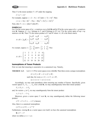
![A.3 Alternating Multilinear Maps
Let f :Vr
! U where V and U are vector spaces over K. [Recall Vr
¼ V V . . . V, r factors.]
(1) The mapping f is said to be multilinear or r-linear if f v1; . . . ; vr
ð Þ is linear as a function of each vj
when the other vi’s are held fixed. That is,
f ð. . . ; vj þ v0
j; . . .Þ ¼ f ð. . . ; vj; . . .Þ þ f ð. . . ; v0
j; . . .Þ
f ð. . . ; kvj; . . .Þ ¼ kf ð. . . ; vj; . . .Þ
where only the jth position changes.
(2) The mapping f is said to be alternating if
f v1; . . . ; vr
ð Þ ¼ 0 whenever vi ¼ vj with i 6¼ j
One can easily show (Prove!) that if f is an alternating multilinear mapping on Vr
, then
f . . . ; vi; . . . ; vj; . . . ¼ f . . . ; vj; . . . ; vi; . . .
That is, if two of the vectors are interchanged, then the associated value changes sign.
EXAMPLE A.3 (Determinants)
The determinant function D:M ! K on the space M of n n matrices may be viewed as an n-variable function
D A
ð Þ ¼ D R1; R2; . . . ; Rn
ð Þ
defined on the rows R1; R2; . . . ; Rn of A. Recall (Chapter 8) that, in this context, D is both n-linear and alternating.
We now need some additional notation. Let K ¼ k1; k2; . . . ; kr
½ denote an r-list (r-tuple) of elements
from In ¼ 1; 2; . . . ; n
ð Þ. We will then use the following notation where the vk’s denote vectors and the
aik’s denote scalars:
vK ¼ ðvk1
; vk2
; . . . ; vkr
Þ and aK ¼ a1k1
a2k2
. . . arkr
Note vK is a list of r vectors, and aK is a product of r scalars.
Now suppose the elements in K ¼ k1; k2; . . . ; kr
½ are distinct. Then K is a permutation sK of an r-list
J ¼ i1; i2; . . . ; ir
½ in standard form, that is, where i1 i2 . . . ir. The number of such standard-form
r-lists J from In is the binomial coefficient:
n
r
¼
n!
r! n r
ð Þ!
[Recall sign sK
ð Þ ¼ 1
ð ÞmK
where mK is the number of interchanges that transforms K into J.]
Now suppose A ¼ aij
is an r n matrix. For a given ordered r-list J, we define
DJ A
ð Þ ¼
a1i1
a1i2
. . . a1ir
a2i1
a2i2
. . . a2ir
ari1
ari2
. . . arir
That is, DJ (A) is the determinant of the r r submatrix of A whose column subscripts belong to J.
Our main theorem below uses the following ‘‘shuffling’’ lemma.
LEMMA A.4 Let V and U be vector spaces over K, and let f :Vr
! U be an alternating r-linear
mapping. Let v1; v2; . . . ; vn be vectors in V and let A ¼ aij
be an r n matrix over K
where r n. For i ¼ 1; 2; . . . ; r, let
ui ¼ ai1vi þ ai2v2 þ þ ainvn
......................
Appendix A Multilinear Products 399](https://image.slidesharecdn.com/linearalgebra4thedition-231030053714-df1faee2/85/Linear_Algebra-_4th_Edition-pdf-406-320.jpg)
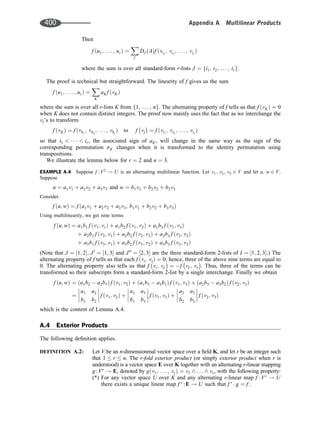
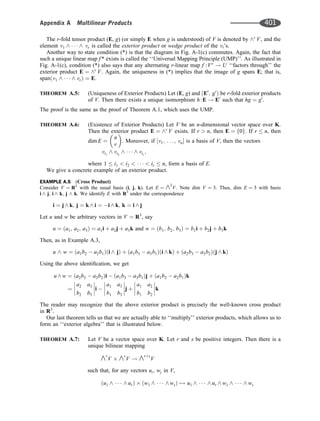
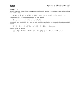
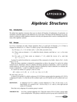
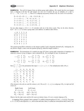
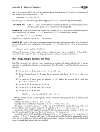
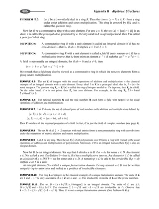
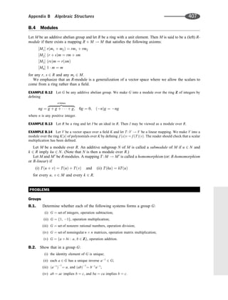
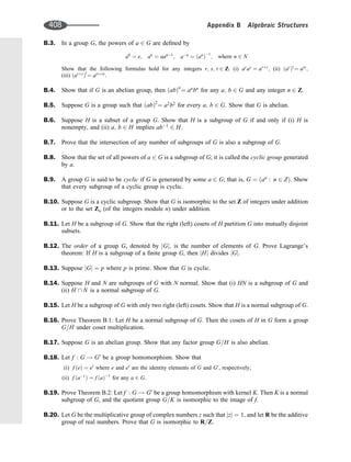
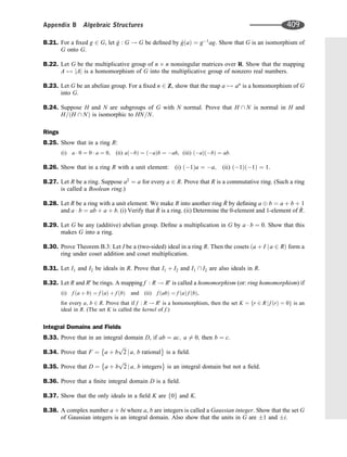
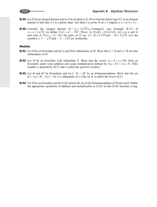
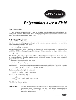
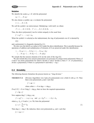
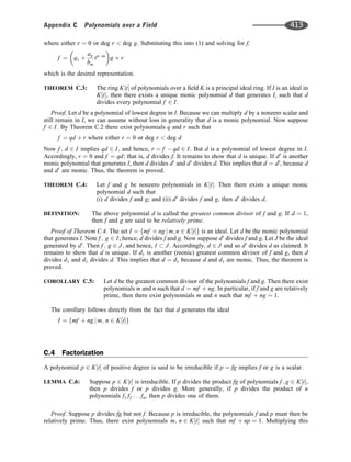
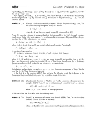
![Odds and Ends
D.1 Introduction
This appendix discusses various topics, such as equivalence relations, determinants and block matrices,
and the generalized MP (Moore–Penrose) inverse.
D.2 Relations and Equivalence Relations
A binary relation or simply relation R from a set A to a set B assigns to each ordered pair a; b
ð Þ 2 A B
exactly one of the following statements:
(i) ‘‘a is related to b,’’ written a R b, (ii) ‘‘a is not related to b’’ written a R b.
A relation from a set A to the same set A is called a relation on A.
Observe that any relation R from A to B uniquely defines a subset ^
R of A B as follows:
^
R ¼ a; b
ð Þja R b
f g
Conversely, any subset ^
R of A B defines a relation from A to B as follows:
a R b if and only if a; b
ð Þ 2 R
In view of the above correspondence between relations from A to B and subsets of A B, we redefine a
relation from A to B as follows:
DEFINITION D.1: A relation R from A to B is a subset of A B.
Equivalence Relations
Consider a nonempty set S. A relation R on S is called an equivalence relation if R is reflexive,
symmetric, and transitive; that is, if R satisfied the following three axioms:
[E1] (Reflexivity) Every a 2 A is related to itself. That is, for every a 2 A, a R a.
[E2] (Symmetry) If a is related to b, then b is related to a. That is, if a R b, then b R a.
[E3] (Transitivity) If a is related to b and b is related to c, then a is related to c. That is,
if a R b and b R c, then a R c:
The general idea behind an equivalence relation is that it is a classification of objects that are in some way
‘‘alike.’’ Clearly, the relation of equality is an equivalence relation. For this reason, one frequently uses ~
or to denote an equivalence relation.
EXAMPLE D.1
(a) In Euclidean geometry, similarity of triangles is an equivalence relation. Specifically, suppose a; b; g are
triangles. Then (i) a is similar to itself. (ii). If a is similar to b, then b is similar to a. (iii) If a is similar to b and b
is similar to g, then a is similar to g.
APPENDIX D
415](https://image.slidesharecdn.com/linearalgebra4thedition-231030053714-df1faee2/85/Linear_Algebra-_4th_Edition-pdf-422-320.jpg)
![(b) The relation of set inclusion is not an equivalence relation. It is reflexive and transitive, but it is not symmetric
because A B does not imply B A.
Equivalence Relations and Partitions
Let S be a nonempty set. Recall first that a partition P of S is a subdivision of S into nonempty,
nonoverlapping subsets; that is, a collection P ¼ fAjg of nonempty subsets of S such that (i) Each a 2 S
belong to one of the Aj, (ii) The sets fAjg are mutually disjoint.
The subsets in a partition P are called cells. Thus, each a 2 S belongs to exactly one of the cells. Also,
any element b 2 Aj is called a representative of the cell Aj, and a subset B of S is called a system of
representatives if B contains exactly one element in each of the cells in fAjg.
Now suppose R is an equivalence relation on the nonempty set S. For each a 2 S, the equivalence class
of a, denoted by [a], is the set of elements of S to which a is related:
a
½ ¼ x j a Rx
f g:
The collection of equivalence classes, denoted by S=R, is called the quotient of S by R:
S=R ¼ a
½ j a 2 S
f g
The fundamental property of an equivalence relation and its quotient set is contained in the following
theorem:
THEOREM D.1: Let R be an equivalence relation on a nonempty set S. Then the quotient set S=R is a
partition of S.
EXAMPLE D.2 Let be the relation on the set Z of integers defined by
x y mod 5
ð Þ
which reads ‘‘x is congruent to y modulus 5’’ and which means that the difference x y is divisible by 5.
Then is an equivalence relation on Z.
Then there are exactly five equivalence classes in the quotient set Z= as follows:
A0 ¼ . . . ; 10; 5; 0; 5; 10; . . .
f g
A1 ¼ . . . ; 9; 4; 1; 6; 11; . . .
f g
A2 ¼ . . . ; 8; 3; 2; 7; 12; . . .
f g
A3 ¼ . . . ; 7; 2; 3; 8; 13; . . .
f g
A4 ¼ . . . ; 6; 1; 4; 9; 14; . . .
f g
Note that any integer x, which can be expressed uniquely in the form x ¼ 5q þ r where 0 r 5, is a
member of the equivalence class Ar where r is the remainder. As expected, the equivalence classes are
disjoint and their union is Z:
Z ¼ A0 [ A1 [ A2 [ A3 [ A4
This quotient set Z= , called the integers modulo 5, is denoted
Z=5Z or simply Z5:
Usually one chooses 0; 1; 2; 3; 4
f g or 2; 1; 0; 1; 2
f g as a system of representatives of the equiva-
lence classes.
Analagously, for any positive integer m, there exists the congruence relation defined by
x y mod m
ð Þ
and the quotient set Z= is called the integers modulo m.
416 Appendix D Odds and Ends](https://image.slidesharecdn.com/linearalgebra4thedition-231030053714-df1faee2/85/Linear_Algebra-_4th_Edition-pdf-423-320.jpg)
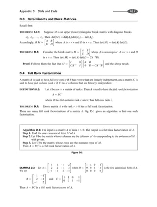
![D.5 Generalized (Moore–Penrose) Inverse
Here we assume that the field of scalars is the complex field C where the matrix AH
is the conjugate
transpose of a matrix A. [If A is a real matrix, then AH
¼ AT
.]
DEFINITION D.3: Let A be an m n matrix over C. A matrix, denoted by Aþ
, is called the
pseudoinverse or Morre–Penrose inverse or MP-inverse of A if A satisfies the
following four equations:
[MP1] AXA ¼ A; [MP3] AX
ð ÞH
¼ AX;
[MP2] XAX ¼ X; [MP4] XA
ð ÞH
¼ XA;
Clearly, Aþ
is an n m matrix. Also, Aþ
¼ A1
if A is nonsingular.
LEMMA D.4: Aþ
is unique (when it exists).
Proof. Suppose X and Y satisfy the four MP equations. Then
AY ¼ AY
ð ÞH
¼ AXAY
ð ÞH
¼ AY
ð ÞH
AX
ð ÞH
¼ AYAX ¼ AYA
ð ÞX ¼ AX
The first and fourth equations use [MP3], and the second and last equations use [MP1]. Similarly,
YA ¼ XA (which uses [MP4] and [MP1]). Then,
Y ¼ YAY ¼ YA
ð ÞY ¼ XA
ð ÞY ¼ X AY
ð Þ ¼ X AX
ð Þ ¼ X
where the first equation uses [MP2].
LEMMA D.5: Aþ
exists for any matrix A.
Fig. D-2 gives an algorithm that finds an MP-inverse for any matrix A.
Combining the above two lemmas we obtain:
THEOREM D.6: Every matrix A over C has a unique Moore–Penrose matrix Aþ
.
There are special cases when A has full-row rank or full-column rank.
THEOREM D.7: Let A be a matrix over C.
(a) If A has full column rank (columns are linearly independent), then
Aþ
¼ AH
A
ð Þ
1
AH
:
(b) If A has full row rank (rows are linearly independent), then Aþ
¼ AH
AAH
ð Þ
1
:
THEOREM D.8: Let A be a matrix over C. Suppose A ¼ BC is a full rank factorization of A. Then
Aþ
¼ Cþ
Bþ
¼ CH
CCH 1
BH
B
1
BH
Moreover, AAþ
¼ BBþ
and Aþ
A ¼ Cþ
C:
Algorithm D-2. Input is an m n matrix A over C or rank r. Output is Aþ
.
Step 1. Interchange rows and columns of A so that PAQ ¼
A11 A12
A21 A22
where A11 is a nonsingular
r r block. [Here P and Q are the products of elementary matrices corresponding to the
interchanges of the rows and columns.]
Step 2. Set B ¼
A11
A21
and C ¼ Ir; A1
11 A12
where Ir is the r r identity matrix.
Step 3. Set Aþ
¼ Q CH
CCH
ð Þ
1
BH
B
ð Þ
1
B11
h i
P:
Figure D-2
418 Appendix D Odds and Ends](https://image.slidesharecdn.com/linearalgebra4thedition-231030053714-df1faee2/85/Linear_Algebra-_4th_Edition-pdf-425-320.jpg)