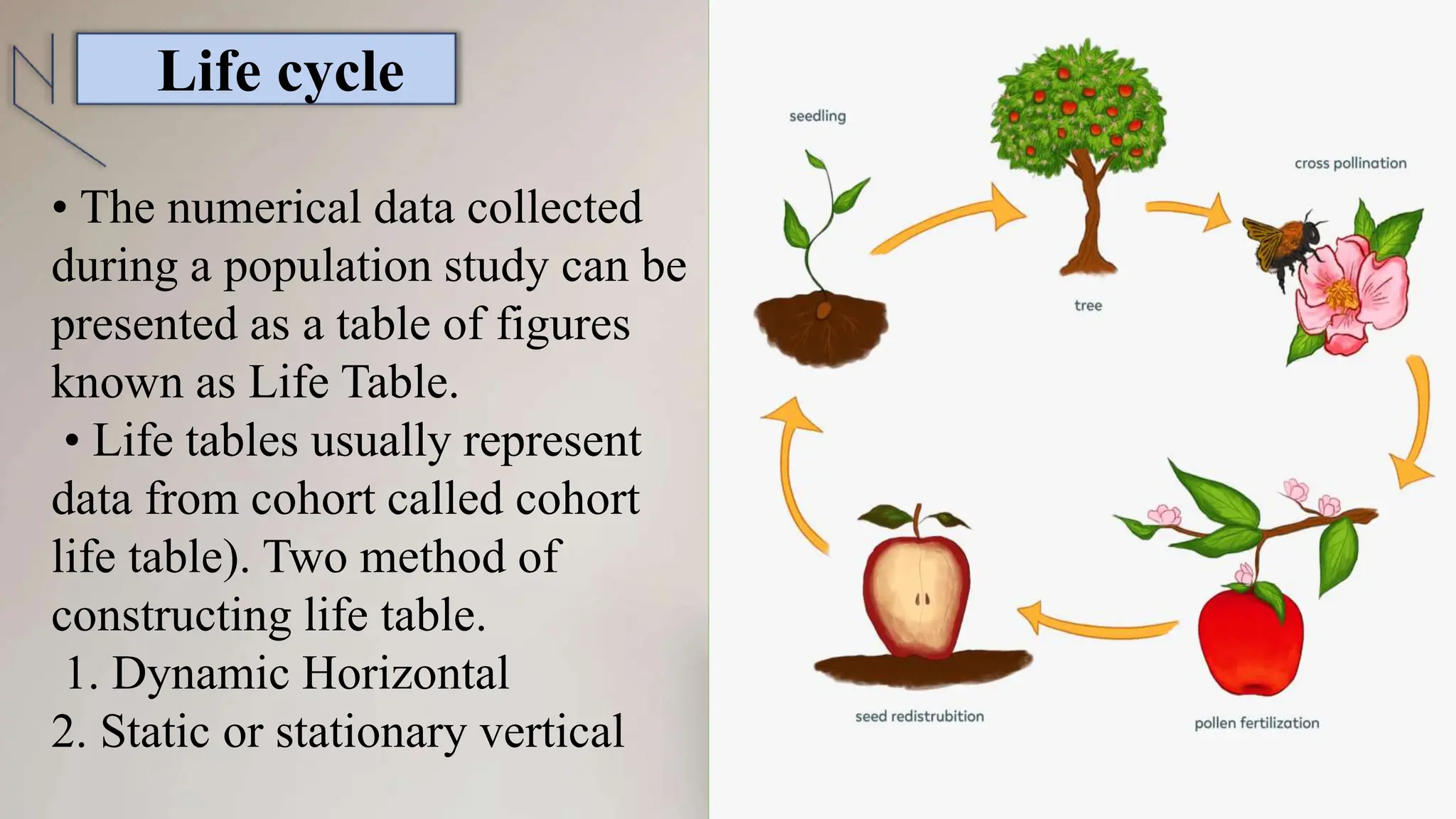
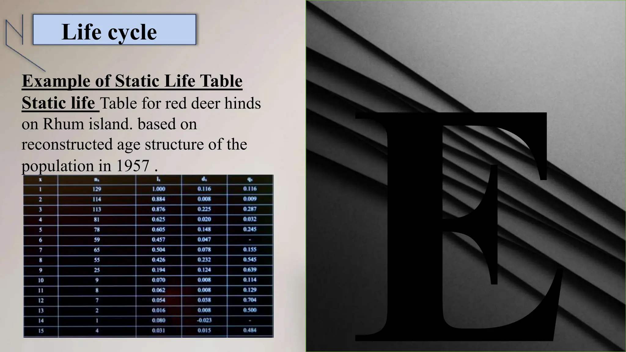
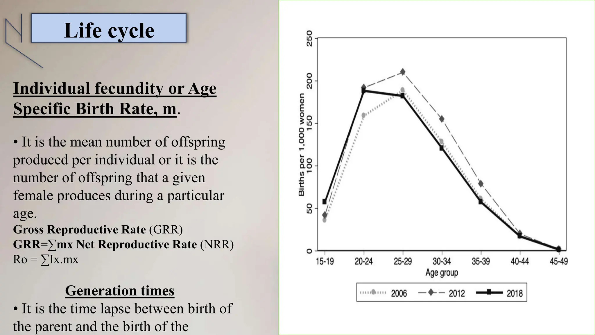
Life cycle
GOVERNMENT E. RAGHAVENDRA RAO PG SCIENCE COLLEGE,
BILASPUR (C.G.)
Department of zoology
Topic – Life table
Guided by -
Mr. Santosh Agrawal
Submitted by - Chitrakanta pendro
M.Sc. III semester
• The numerical data collected
during a population study can be
presented as a table of figures
known as Life Table.
• Life tables usually represent
data from cohort called cohort
life table). Two method of
constructing life table.
1. Dynamic Horizontal
2. Static or stationary vertical
Life cycle
• Dynamic
Horizontal
In this we start with a
known group of individuals
called cohort and observe
bow many die at each age
till all of them die. This
method of constructing life
table is called Dynamic
Horizontal.
Dynamic Horizontal
• Static or stationary
vertical
The other method is called
static or stationary vertical. In
this method a cross section of
population at given time is
taken and its age structure
related observation are taken.
Life
cycle
Example of Cohort Life Table
Where, Age (years) = x Proportion
of original cohort surviving to the
beginning of age class x = lx .
Proportion of original cohort dying
during age class x = dx Mortality
rate = qx
Life cycle
Example of Static Life Table
Static life Table for red deer hinds
on Rhum island. based on
reconstructed age structure of the
population in 1957 .
Life cycle
Individual fecundity or Age
Specific Birth Rate, m.
• It is the mean number of offspring
produced per individual or it is the
number of offspring that a given
female produces during a particular
age.
Gross Reproductive Rate (GRR)
GRR=∑mx Net Reproductive Rate (NRR)
Ro = ∑Ix.mx
Generation times
• It is the time lapse between birth of
the parent and the birth of the
Life cycle
Gross Reproductive Rate (GRR)
20.0 Net Reproductive Rate
(NRR), R = 11.44
Life cycle
2. Survivorship Curve
• Cohort life table data are often shown
as a survivorship curve for a particular
particular population
• This is a graph showing the number of
individuals which survives through each
phase of life
• Pearl described 3 types of
survivorship curve
l. Type I or Convex Curve .
2. Type II or Diagonal straight line .
Survival curve
• Type I or Convex Curve:
In such population, there is little mortality until some age and then fairly steep mortality is
observed for example modem industrialized man, and many species of large animals.
• Type II or Diagonal straight line:
In such populations, mortality is constant at all age groups for example birds, rabbit and
mice, hydra, animals related to jellyfish etc.
• Type III or Concave curve
Such populations are characterized by high mortality during the young stage but
lower or nearly constant in the adult e.g. Oyster, most trees, many fishes and insects.
This appears to be the most common survivorship curve among animals and plants in
nature These types of survivorship curve are useful generalizations, but in practice,
patterns of survival are usually more complex. Thus, in a population of Erophila
verna, a very short-lived annual plant inhabiting sand dunes, survival can follow a
type I curve when the plants grow at low densities; a type II curve, at least until the
Survival
curve
Reference
 E- P ODUM
 BROTANICA ENCYCLOPEDIA
 SOME ONLINE ARTICLES
https://www.youtube.com
/
 https://www.google.
com/
Life cycle
Thank
Life cycle

Life table / life cycle (Chitra ).pptx

  • 1.
    Life cycle GOVERNMENT E.RAGHAVENDRA RAO PG SCIENCE COLLEGE, BILASPUR (C.G.) Department of zoology Topic – Life table Guided by - Mr. Santosh Agrawal Submitted by - Chitrakanta pendro M.Sc. III semester
  • 2.
    • The numericaldata collected during a population study can be presented as a table of figures known as Life Table. • Life tables usually represent data from cohort called cohort life table). Two method of constructing life table. 1. Dynamic Horizontal 2. Static or stationary vertical Life cycle
  • 3.
    • Dynamic Horizontal In thiswe start with a known group of individuals called cohort and observe bow many die at each age till all of them die. This method of constructing life table is called Dynamic Horizontal. Dynamic Horizontal
  • 4.
    • Static orstationary vertical The other method is called static or stationary vertical. In this method a cross section of population at given time is taken and its age structure related observation are taken. Life cycle
  • 5.
    Example of CohortLife Table Where, Age (years) = x Proportion of original cohort surviving to the beginning of age class x = lx . Proportion of original cohort dying during age class x = dx Mortality rate = qx Life cycle
  • 6.
    Example of StaticLife Table Static life Table for red deer hinds on Rhum island. based on reconstructed age structure of the population in 1957 . Life cycle
  • 7.
    Individual fecundity orAge Specific Birth Rate, m. • It is the mean number of offspring produced per individual or it is the number of offspring that a given female produces during a particular age. Gross Reproductive Rate (GRR) GRR=∑mx Net Reproductive Rate (NRR) Ro = ∑Ix.mx Generation times • It is the time lapse between birth of the parent and the birth of the Life cycle
  • 8.
    Gross Reproductive Rate(GRR) 20.0 Net Reproductive Rate (NRR), R = 11.44 Life cycle
  • 9.
    2. Survivorship Curve •Cohort life table data are often shown as a survivorship curve for a particular particular population • This is a graph showing the number of individuals which survives through each phase of life • Pearl described 3 types of survivorship curve l. Type I or Convex Curve . 2. Type II or Diagonal straight line . Survival curve
  • 10.
    • Type Ior Convex Curve: In such population, there is little mortality until some age and then fairly steep mortality is observed for example modem industrialized man, and many species of large animals. • Type II or Diagonal straight line: In such populations, mortality is constant at all age groups for example birds, rabbit and mice, hydra, animals related to jellyfish etc. • Type III or Concave curve Such populations are characterized by high mortality during the young stage but lower or nearly constant in the adult e.g. Oyster, most trees, many fishes and insects. This appears to be the most common survivorship curve among animals and plants in nature These types of survivorship curve are useful generalizations, but in practice, patterns of survival are usually more complex. Thus, in a population of Erophila verna, a very short-lived annual plant inhabiting sand dunes, survival can follow a type I curve when the plants grow at low densities; a type II curve, at least until the Survival curve
  • 11.
    Reference  E- PODUM  BROTANICA ENCYCLOPEDIA  SOME ONLINE ARTICLES https://www.youtube.com /  https://www.google. com/ Life cycle
  • 12.