The document provides an overview of adversarial machine learning, focusing on key concepts in machine learning and deep learning, including supervised, unsupervised, and reinforcement learning methods. It delineates various classification techniques, neural network architectures, and the role of deep learning in extracting complex data representations. Additionally, the document addresses limitations like the no-free-lunch theorem and the representational power of neural networks.

1. CS 404/504
Special Topics: Adversarial Machine
Learning
Dr. Alex Vakanski

2. 2
CS 404/504, Fall 2021
Lecture 2
Deep Learning Overview

3. 3
CS 404/504, Fall 2021
Lecture Outline
• Machine learning basics
 Supervised and unsupervised learning
 Linear and non-linear classification methods
• Introduction to deep learning
• Elements of neural networks (NNs)
 Activation functions
• Training NNs
 Gradient descent
 Regularization methods
• NN architectures
 Convolutional NNs
 Recurrent NNs

4. 4
CS 404/504, Fall 2021
Machine Learning Basics
• Artificial Intelligence is a scientific field concerned with the development of
algorithms that allow computers to learn without being explicitly programmed
• Machine Learning is a branch of Artificial Intelligence, which focuses on
methods that learn from data and make predictions on unseen data
Machine Learning Basics
Labeled Data
Labeled Data
Machine Learning
algorithm
Learned
model
Predictio
n
Training
Prediction
Picture from: Ismini Lourentzou – Introduction to Deep Learning

5. 5
CS 404/504, Fall 2021
Machine Learning Types
• Supervised: learning with labeled data
 Example: email classification, image classification
 Example: regression for predicting real-valued outputs
• Unsupervised: discover patterns in unlabeled data
 Example: cluster similar data points
• Reinforcement learning: learn to act based on feedback/reward
 Example: learn to play Go
Machine Learning Basics
class A
class B
Classification Regression Clustering
Slide credit: Ismini Lourentzou – Introduction to Deep Learning

6. 6
CS 404/504, Fall 2021
Supervised Learning
• Supervised learning categories and techniques
 Numerical classifier functions
o Linear classifier, perceptron, logistic regression, support vector machines (SVM), neural
networks
 Parametric (probabilistic) functions
o Naïve Bayes, Gaussian discriminant analysis (GDA), hidden Markov models (HMM),
probabilistic graphical models
 Non-parametric (instance-based) functions
o k-nearest neighbors, kernel regression, kernel density estimation, local regression
 Symbolic functions
o Decision trees, classification and regression trees (CART)
 Aggregation (ensemble) learning
o Bagging, boosting (Adaboost), random forest
Machine Learning Basics
Slide credit: Y-Fan Chang – An Overview of Machine Learning

7. 7
CS 404/504, Fall 2021
Unsupervised Learning
• Unsupervised learning categories and techniques
 Clustering
o k-means clustering
o Mean-shift clustering
o Spectral clustering
 Density estimation
o Gaussian mixture model (GMM)
o Graphical models
 Dimensionality reduction
o Principal component analysis (PCA)
o Factor analysis
Machine Learning Basics
Slide credit: Y-Fan Chang – An Overview of Machine Learning

8. 8
CS 404/504, Fall 2021
Nearest Neighbor Classifier
• Nearest Neighbor – for each test data point, assign the class label of the nearest
training data point
 Adopt a distance function to find the nearest neighbor
o Calculate the distance to each data point in the training set, and assign the class of the nearest
data point (minimum distance)
 It does not require learning a set of weights
Machine Learning Basics
Test
example
Training
examples
from class 1
Training
examples
from class 2
Picture from: James Hays – Machine Learning Overview

9. 9
CS 404/504, Fall 2021
Nearest Neighbor Classifier
• For image classification, the distance between all pixels is calculated (e.g., using
ℓ1 norm, or ℓ2 norm)
 Accuracy on CIFAR-10: 38.6%
• Disadvantages:
 The classifier must remember all training data and store it for future comparisons with
the test data
 Classifying a test image is expensive since it requires a comparison to all training
images
Machine Learning Basics
Picture from: https://cs231n.github.io/classification/
ℓ1 norm
(Manhattan distance)

10. 10
CS 404/504, Fall 2021
k-Nearest Neighbors Classifier
• k-Nearest Neighbors approach considers multiple neighboring data points to
classify a test data point
 E.g., 3-nearest neighbors
o The test example in the figure is the + mark
o The class of the test example is obtained by voting (based on the distance to the 3 closest
points)
Machine Learning Basics
x x
x
x
x
x
x
x
o
o
o
o
o
o
o
x2
x1
o
o
x
+
+
Picture from: James Hays – Machine Learning Overview

11. 11
CS 404/504, Fall 2021
Linear Classifier
• Linear classifier
 Find a linear function f of the inputs xi that separates the classes
𝑓 𝑥𝑖, 𝑊, 𝑏 = 𝑊𝑥𝑖 + 𝑏
 Use pairs of inputs and labels to find the weights matrix W and the bias vector b
o The weights and biases are the parameters of the function f
 Several methods have been used to find the optimal set of parameters of a linear
classifier
o A common method of choice is the Perceptron algorithm, where the parameters are updated
until a minimal error is reached (single layer, does not use backpropagation)
 Linear classifier is a simple approach, but it is a building block of advanced
classification algorithms, such as SVM and neural networks
o Earlier multi-layer neural networks were referred to as multi-layer perceptrons (MLPs)
Machine Learning Basics

12. 12
CS 404/504, Fall 2021
Linear Classifier
• The decision boundary is linear
 A straight line in 2D, a flat plane in 3D, a hyperplane in 3D and
higher dimensional space
• Example: classify an input image
 The selected parameters in this example are not good, because the
predicted cat score is low
Machine Learning Basics
Picture from: https://cs231n.github.io/classification/

13. 13
CS 404/504, Fall 2021
Support Vector Machines
• Support vector machines (SVM)
 How to find the best decision boundary?
o All lines in the figure correctly separate the 2 classes
o The line that is farthest from all training examples
will have better generalization capabilities
 SVM solves an optimization problem:
o First, identify a decision boundary that correctly
classifies the examples
Machine Learning Basics
o Next, increase the geometric margin between the
boundary and all examples
 The data points that define the maximum
margin width are called support vectors
 Find W and b by solving:

14. 14
CS 404/504, Fall 2021
Linear vs Non-linear Techniques
• Linear classification techniques
 Linear classifier
 Perceptron
 Logistic regression
 Linear SVM
 Naïve Bayes
• Non-linear classification techniques
 k-nearest neighbors
 Non-linear SVM
 Neural networks
 Decision trees
 Random forest
Linear vs Non-linear Techniques

15. 15
CS 404/504, Fall 2021
Linear vs Non-linear Techniques
• For some tasks, input data
can be linearly separable,
and linear classifiers can be
suitably applied
• For other tasks, linear
classifiers may have
difficulties to produce
adequate decision
boundaries
Linear vs Non-linear Techniques
Picture from: Y-Fan Chang – An Overview of Machine Learning

16. 16
CS 404/504, Fall 2021
Non-linear Techniques
• Non-linear classification
 Features 𝑧𝑖 are obtained as non-linear functions of the inputs 𝑥𝑖
 It results in non-linear decision boundaries
 Can deal with non-linearly separable data
Linear vs Non-linear Techniques
Picture from: Y-Fan Chang – An Overview of Machine Learning
Inputs: 𝑥𝑖 = 𝑥𝑛1 𝑥𝑛2
Features: 𝑧𝑖 = 𝑥𝑛1 𝑥𝑛2 𝑥𝑛1 ∙ 𝑥𝑛2 𝑥𝑛1
2
𝑥𝑛2
2
Outputs: 𝑓 𝑥𝑖, 𝑊, 𝑏 = 𝑊𝑧𝑖 + 𝑏

17. 17
CS 404/504, Fall 2021
Non-linear Support Vector Machines
• Non-linear SVM
 The original input space is mapped to a higher-dimensional feature space where the
training set is linearly separable
 Define a non-linear kernel function to calculate a non-linear decision boundary in the
original feature space
Linear vs Non-linear Techniques
Φ: 𝑥 ↦ 𝜙 𝑥
Picture from: James Hays – Machine Learning Overview

18. 18
CS 404/504, Fall 2021
Binary vs Multi-class Classification
• A classification problem with only 2 classes is referred to as binary classification
 The output labels are 0 or 1
 E.g., benign or malignant tumor, spam or no-spam email
• A problem with 3 or more classes is referred to as multi-class classification
Binary vs Multi-class Classification

19. 19
CS 404/504, Fall 2021
Binary vs Multi-class Classification
• Both the binary and multi-class classification problems can be linearly or non-
linearly separated
 Figure: linearly and non-linearly separated data for binary classification problem
Binary vs Multi-class Classification

20. 20
CS 404/504, Fall 2021
Computer Vision Tasks
• Computer vision has been the primary area of interest for ML
• The tasks include: classification, localization, object detection, instance
segmentation
Machine Learning Basics
Picture from: Fie-Fei Li, Andrej Karpathy, Justin Johnson – Understanding and Visualizing CNNs

21. 21
CS 404/504, Fall 2021
No-Free-Lunch Theorem
• Wolpert (2002) - The Supervised Learning No-Free-Lunch Theorems
• The derived classification models for supervised learning are simplifications of
the reality
 The simplifications are based on certain assumptions
 The assumptions fail in some situations
o E.g., due to inability to perfectly estimate ML model parameters from limited data
• In summary, No-Free-Lunch Theorem states:
 No single classifier works the best for all possible problems
 Since we need to make assumptions to generalize
Machine Learning Basics

22. 22
CS 404/504, Fall 2021
ML vs. Deep Learning
• Conventional machine learning methods rely on human-designed feature
representations
 ML becomes just optimizing weights to best make a final prediction
Introduction to Deep Learning
Picture from: Ismini Lourentzou – Introduction to Deep Learning

23. 23
CS 404/504, Fall 2021
ML vs. Deep Learning
• Deep learning (DL) is a machine learning subfield that uses multiple layers for
learning data representations
 DL is exceptionally effective at learning patterns
Introduction to Deep Learning
Picture from: https://www.xenonstack.com/blog/static/public/uploads/media/machine-learning-vs-deep-learning.png

24. 24
CS 404/504, Fall 2021
ML vs. Deep Learning
• DL applies a multi-layer process for learning rich hierarchical features (i.e., data
representations)
 Input image pixels → Edges → Textures → Parts → Objects
Introduction to Deep Learning
Low-Level
Features
Mid-Level
Features
Output
High-Level
Features
Trainable
Classifier
Slide credit: Param Vir Singh – Deep Learning

25. 25
CS 404/504, Fall 2021
Why is DL Useful?
• DL provides a flexible, learnable framework for representing visual, text,
linguistic information
 Can learn in supervised and unsupervised manner
• DL represents an effective end-to-end learning system
• Requires large amounts of training data
• Since about 2010, DL has outperformed other ML techniques
 First in vision and speech, then NLP, and other applications
Introduction to Deep Learning

26. 26
CS 404/504, Fall 2021
Representational Power
• NNs with at least one hidden layer are universal approximators
 Given any continuous function h(x) and some 𝜖 > 0, there exists a NN with one
hidden layer (and with a reasonable choice of non-linearity) described with the
function f(x), such that ∀𝑥, ℎ 𝑥 − 𝑓(𝑥) < 𝜖
 I.e., NN can approximate any arbitrary complex continuous function
Introduction to Deep Learning
• NNs use nonlinear mapping of the inputs x to the
outputs f(x) to compute complex decision boundaries
• But then, why use deeper NNs?
 The fact that deep NNs work better is an empirical
observation
 Mathematically, deep NNs have the same
representational power as a one-layer NN

27. 27
CS 404/504, Fall 2021
Introduction to Neural Networks
• Handwritten digit recognition (MNIST dataset)
 The intensity of each pixel is considered an input element
 Output is the class of the digit
Introduction to Neural Networks
Input
16 x 16 = 256
1
x
2
x
256
x
……
Ink → 1
No ink → 0
……
y1
y2
y10
Each dimension represents the
confidence of a digit
is 1
is 2
is 0
……
0.1
0.7
0.2
The image is “2”
Output
Slide credit: Hung-yi Lee – Deep Learning Tutorial

28. 28
CS 404/504, Fall 2021
Introduction to Neural Networks
• Handwritten digit recognition
Introduction to Neural Networks
Machine “2”
1
x
2
x
256
x
……
……
y1
y2
y10
𝑓: 𝑅256 → 𝑅10
The function 𝑓 is represented by a neural network
Slide credit: Hung-yi Lee – Deep Learning Tutorial

29. 29
CS 404/504, Fall 2021
Elements of Neural Networks
• NNs consist of hidden layers with neurons (i.e., computational units)
• A single neuron maps a set of inputs into an output number, or 𝑓: 𝑅𝐾 → 𝑅
Introduction to Neural Networks
b
w
a
w
a
w
a
z K
K 



 
2
2
1
1
z
1
w
2
w
K
w
…
1
a
2
a
K
a

b
 
z

bias
a
Activation
function
weights
𝑎 = 𝜎 𝑧
input
output
…
Slide credit: Hung-yi Lee – Deep Learning Tutorial

30. 30
CS 404/504, Fall 2021
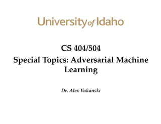
Elements of Neural Networks
• A NN with one hidden layer and one output layer
Introduction to Neural Networks
𝒉
𝒚
𝒙
𝒉𝒊𝒅𝒅𝒆𝒏 𝒍𝒂𝒚𝒆𝒓 𝒉 = 𝝈(𝐖𝟏𝒙 + 𝒃𝟏)
𝒐𝒖𝒕𝒑𝒖𝒕 𝒍𝒂𝒚𝒆𝒓 𝒚 = 𝝈(𝑾𝟐𝒉 + 𝒃𝟐)
Weights Biases
Activation functions
4 + 2 = 6 neurons (not counting inputs)
[3 × 4] + [4 × 2] = 20 weights
4 + 2 = 6 biases
26 learnable parameters
Slide credit: Ismini Lourentzou – Introduction to Deep Learning

31. 31
CS 404/504, Fall 2021
Elements of Neural Networks
• A neural network playground link
Introduction to Neural Networks

32. 32
CS 404/504, Fall 2021
Elements of Neural Networks
• Deep NNs have many hidden layers
 Fully-connected (dense) layers (a.k.a. Multi-Layer Perceptron or MLP)
 Each neuron is connected to all neurons in the succeeding layer
Introduction to Neural Networks
Output Layer
Hidden Layers
Input Layer
Input Output
1
x
2
x
Layer 1
……
N
x
……
Layer 2
……
Layer L
……
……
……
……
……
y1
y2
yM
Slide credit: Hung-yi Lee – Deep Learning Tutorial

33. 33
CS 404/504, Fall 2021
Elements of Neural Networks
• A simple network, toy example
Introduction to Neural Networks
 
z

z
  z
e
z 


1
1

Sigmoid Function
1
-1
1
-2
1
-1
1
0
4
-2
0.98
0.12
1 ∙ 1 + −1 ∙ −2 + 1 = 4
1 ∙ −1 + −1 ∙ 1 + 0 =-2
Slide credit: Hung-yi Lee – Deep Learning Tutorial

34. 34
CS 404/504, Fall 2021
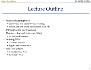
Elements of Neural Networks
• A simple network, toy example (cont’d)
 For an input vector [1 −1]𝑇
, the output is [0.62 0.83]𝑇
Introduction to Neural Networks
1
-2
1
-1
1
0
4
-2
0.98
0.12
2
-1
-1
-2
3
-1
4
-1
0.86
0.11
0.62
0.83
0
0
-2
2
1
-1
𝑓: 𝑅2
→ 𝑅2 𝑓
1
−1
=
0.62
0.83
Slide credit: Hung-yi Lee – Deep Learning Tutorial

35. 35
CS 404/504, Fall 2021
Matrix Operation
• Matrix operations are helpful when working with multidimensional inputs and
outputs
Introduction to Neural Networks
1
-2
1
-1
1
0
4
-2
0.98
0.12
1
-1
Slide credit: Hung-yi Lee – Deep Learning Tutorial
𝜎
1
−1
1 −2
−1 1 +
1
0
0.98
0.12
=
4
−2
b
W x +
𝜎 = a

36. 36
CS 404/504, Fall 2021
Matrix Operation
• Multilayer NN, matrix calculations for the first layer
 Input vector x, weights matrix W1, bias vector b1, output vector a1
Introduction to Neural Networks
1
x
2
x
……
N
x
……
……
……
……
……
……
……
y1
y2
yM
W1
x a1
b1
W1 x +
= 𝜎
b1
a1
Slide credit: Hung-yi Lee – Deep Learning Tutorial

37. 37
CS 404/504, Fall 2021
Matrix Operation
• Multilayer NN, matrix calculations for all layers
Introduction to Neural Networks
1
x
2
x
……
N
x
……
……
……
……
……
……
……
y1
y2
yM
W1 W2 WL
b2 bL
x a1
a2 y
b1
W1 x +
𝜎
b2
W2 a1 +
𝜎
bL
WL +
𝜎 aL-1
b1
Slide credit: Hung-yi Lee – Deep Learning Tutorial

38. 38
CS 404/504, Fall 2021
Matrix Operation
• Multilayer NN, function f maps inputs x to outputs y, i.e., 𝑦 = 𝑓(𝑥)
Introduction to Neural Networks
= 𝜎 𝜎
1
x
2
x
……
N
x
……
……
……
……
……
……
……
y1
y2
yM
W1 W2 WL
b2 bL
x a1
a2 y
y = 𝑓 x b1
W1 x +
𝜎 b2
W2
+ bL
WL
+
…
b1
…
Slide credit: Hung-yi Lee – Deep Learning Tutorial

39. 39
CS 404/504, Fall 2021
Softmax Layer
• In multi-class classification tasks, the output layer is typically a softmax layer
 I.e., it employs a softmax activation function
 If a layer with a sigmoid activation function is used as the output layer instead, the
predictions by the NN may not be easy to interpret
o Note that an output layer with sigmoid activations can still be used for binary classification
Introduction to Neural Networks
Slide credit: Hung-yi Lee – Deep Learning Tutorial
A Layer with Sigmoid Activations
 
1
1 z
y 

 
2
2 z
y 

 
3
3 z
y 

1
z
2
z
3
z



3
-3
1
0.95
0.05
0.73

40. 40
CS 404/504, Fall 2021
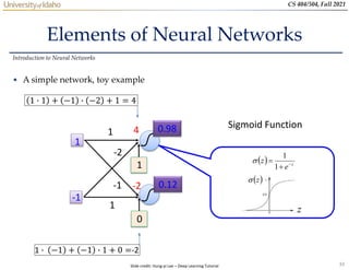
Softmax Layer
• The softmax layer applies softmax activations to output
a probability value in the range [0, 1]
 The values z inputted to the softmax layer are referred to as
logits
Introduction to Neural Networks
1
z
2
z
3
z
A Softmax Layer
e
e
e
1
z
e
2
z
e
3
z
e




3
1
1
1
j
z
z j
e
e
y


3
1
j
z j
e



3
-3
1 2.7
20
0.05
0.88
0.12
≈0



3
1
2
2
j
z
z j
e
e
y



3
1
3
3
j
z
z j
e
e
y
Probability:
 0 < 𝑦𝑖 < 1
 𝑖 𝑦𝑖 = 1
Slide credit: Hung-yi Lee – Deep Learning Tutorial

41. 41
CS 404/504, Fall 2021
Activation Functions
• Non-linear activations are needed to learn complex (non-linear) data
representations
 Otherwise, NNs would be just a linear function (such as W1W2𝑥 = 𝑊𝑥)
 NNs with large number of layers (and neurons) can approximate more complex
functions
o Figure: more neurons improve representation (but, may overfit)
Introduction to Neural Networks
Picture from: http://cs231n.github.io/assets/nn1/layer_sizes.jpeg

42. 42
CS 404/504, Fall 2021
Activation: Sigmoid
• Sigmoid function σ: takes a real-valued number and “squashes” it into the range
between 0 and 1
 The output can be interpreted as the firing rate of a biological neuron
o Not firing = 0; Fully firing = 1
 When the neuron’s activation are 0 or 1, sigmoid neurons saturate
o Gradients at these regions are almost zero (almost no signal will flow)
 Sigmoid activations are less common in modern NNs
Introduction to Neural Networks
Slide credit: Ismini Lourentzou – Introduction to Deep Learning
ℝ𝑛
→ 0,1
𝑥
𝑓 𝑥

43. 43
CS 404/504, Fall 2021
Activation: Tanh
• Tanh function: takes a real-valued number and “squashes” it into range between
-1 and 1
 Like sigmoid, tanh neurons saturate
 Unlike sigmoid, the output is zero-centered
o It is therefore preferred than sigmoid
 Tanh is a scaled sigmoid: tanh(𝑥) = 2 ∙ 𝜎(2𝑥) − 1
Introduction to Neural Networks
Slide credit: Ismini Lourentzou – Introduction to Deep Learning
ℝ𝑛 → −1,1
𝑥
𝑓 𝑥

44. 44
CS 404/504, Fall 2021
Activation: ReLU
• ReLU (Rectified Linear Unit): takes a real-valued number and thresholds it at
zero
𝑓 𝑥 = max(0, 𝑥)
Introduction to Neural Networks
 Most modern deep NNs use ReLU
activations
 ReLU is fast to compute
o Compared to sigmoid, tanh
o Simply threshold a matrix at zero
 Accelerates the convergence of gradient
descent
o Due to linear, non-saturating form
 Prevents the gradient vanishing problem
ℝ𝑛 → ℝ+
𝑛
𝑥
𝑓 𝑥

45. 45
CS 404/504, Fall 2021
Activation: Leaky ReLU
• The problem of ReLU activations: they can “die”
 ReLU could cause weights to update in a way that the gradients can become zero and
the neuron will not activate again on any data
 E.g., when a large learning rate is used
• Leaky ReLU activation function is a variant of ReLU
 Instead of the function being 0 when 𝑥 < 0, a leaky ReLU has a small negative slope
(e.g., α = 0.01, or similar)
Introduction to Neural Networks
𝑓 𝑥 =
𝛼𝑥 for 𝑥 < 0
𝑥 for 𝑥 ≫ 0
 This resolves the dying ReLU problem
 Most current works still use ReLU
o With a proper setting of the learning rate,
the problem of dying ReLU can be avoided

46. 46
CS 404/504, Fall 2021
Activation: Linear Function
• Linear function means that the output signal is proportional to the input signal
to the neuron
Introduction to Neural Networks
𝑓 𝑥 = 𝑐𝑥
ℝ𝑛 → ℝ𝑛
 If the value of the constant c is 1, it is also
called identity activation function
 This activation type is used in regression
problems
o E.g., the last layer can have linear activation
function, in order to output a real number
(and not a class membership)

47. 47
CS 404/504, Fall 2021
Training NNs
• The network parameters 𝜃 include the weight matrices and bias vectors from all
layers
 Often, the model parameters 𝜃 are referred to as weights
• Training a model to learn a set of parameters 𝜃 that are optimal (according to a
criterion) is one of the greatest challenges in ML
Training Neural Networks
𝜃 = 𝑊1
, 𝑏1
, 𝑊2
, 𝑏2
, ⋯ 𝑊𝐿
, 𝑏𝐿
16 x 16 = 256
1
x
2
x
……
256
x
……
……
……
……
……
y1
y2
y10
0.1
0.7
0.2
is 1
is 2
is 0
Softmax
Slide credit: Hung-yi Lee – Deep Learning Tutorial

48. 48
CS 404/504, Fall 2021
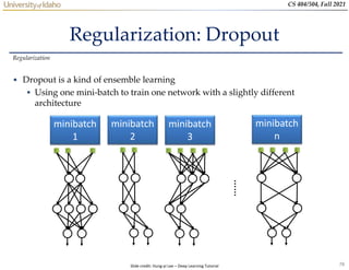
Training NNs
• Data preprocessing - helps convergence during training
 Mean subtraction, to obtain zero-centered data
o Subtract the mean for each individual data dimension (feature)
 Normalization
o Divide each feature by its standard deviation
– To obtain standard deviation of 1 for each data dimension (feature)
o Or, scale the data within the range [0,1] or [-1, 1]
– E.g., image pixel intensities are divided by 255 to be scaled in the [0,1] range
Training Neural Networks
Picture from: https://cs231n.github.io/neural-networks-2/

49. 49
CS 404/504, Fall 2021
Training NNs
• To train a NN, set the parameters 𝜃 such that for a training subset of images, the
corresponding elements in the predicted output have maximum values
Training Neural Networks
y1 has the maximum value
Input:
y2 has the maximum value
Input:
.
.
.
Input: y9 has the maximum value
Input: y10 has the maximum value
Slide credit: Hung-yi Lee – Deep Learning Tutorial

50. 50
CS 404/504, Fall 2021
Training NNs
• Define a loss function/objective function/cost function ℒ 𝜃 that calculates the
difference (error) between the model prediction and the true label
 E.g., ℒ 𝜃 can be mean-squared error, cross-entropy, etc.
Training Neural Networks
1
x
2
x
……
256
x
……
……
……
……
……
y1
y2
y10
Cost
0.2
0.3
0.5
……
1
0
0
……
True label “1”
ℒ(𝜃)
……
Slide credit: Hung-yi Lee – Deep Learning Tutorial

51. 51
CS 404/504, Fall 2021
Training NNs
• For a training set of 𝑁 images, calculate the total loss overall all images: ℒ 𝜃 =
𝑛=1
𝑁
ℒ𝑛 𝜃
• Find the optimal parameters 𝜃∗
that minimize the total loss ℒ 𝜃
Training Neural Networks
x1
x2
xN
NN
NN
NN
……
……
y1
y2
yN
𝑦1
𝑦2
𝑦𝑁
ℒ1 𝜃
……
……
x3 NN y3
𝑦3
ℒ2 𝜃
ℒ3 𝜃
ℒ𝑛 𝜃
Slide credit: Hung-yi Lee – Deep Learning Tutorial

52. 52
CS 404/504, Fall 2021
Loss Functions
• Classification tasks
Training Neural Networks
Slide credit: Ismini Lourentzou – Introduction to Deep Learning
Training
examples
Output
Layer
Softmax Activations
[maps to a probability distribution]
Loss function Cross-entropy ℒ 𝜃 = −
1
𝑁
𝑖=1
𝑁
𝑘=1
𝐾
𝑦𝑘
(𝑖)
log 𝑦𝑘
(𝑖)
+ 1 − 𝑦𝑘
(𝑖)
log 1 − 𝑦𝑘
𝑖
Pairs of 𝑁 inputs 𝑥𝑖 and ground-truth class labels 𝑦𝑖
Ground-truth class labels 𝑦𝑖 and model predicted class labels 𝑦𝑖

53. 53
CS 404/504, Fall 2021
Loss Functions
• Regression tasks
Training Neural Networks
Slide credit: Ismini Lourentzou – Introduction to Deep Learning
Training
examples
Output
Layer
Loss function
Mean Squared Error ℒ 𝜃 =
1
𝑛
𝑖=1
𝑛
𝑦(𝑖) − 𝑦(𝑖) 2
Linear (Identity) or Sigmoid Activation
Mean Absolute Error ℒ 𝜃 =
1
𝑛
𝑖=1
𝑛
𝑦(𝑖) − 𝑦(𝑖)
Pairs of 𝑁 inputs 𝑥𝑖 and ground-truth output values 𝑦𝑖

54. 54
CS 404/504, Fall 2021
Training NNs
• Optimizing the loss function ℒ 𝜃
 Almost all DL models these days are trained with a variant of the gradient descent
(GD) algorithm
 GD applies iterative refinement of the network parameters 𝜃
 GD uses the opposite direction of the gradient of the loss with respect to the NN
parameters (i.e.,𝛻ℒ 𝜃 = 𝜕ℒ 𝜕𝜃𝑖 ) for updating 𝜃
o The gradient of the loss function 𝛻ℒ 𝜃 gives the direction of fastest increase of the loss
function ℒ 𝜃 when the parameters 𝜃 are changed
Training Neural Networks
ℒ 𝜃
𝜃𝑖
𝜕ℒ
𝜕𝜃𝑖

55. 55
CS 404/504, Fall 2021
Gradient Descent Algorithm
• Steps in the gradient descent algorithm:
1. Randomly initialize the model parameters, 𝜃0
2. Compute the gradient of the loss function at the initial parameters 𝜃0
: 𝛻ℒ 𝜃0
3. Update the parameters as: 𝜃𝑛𝑒𝑤 = 𝜃0 − 𝛼𝛻ℒ 𝜃0
o Where α is the learning rate
4. Go to step 2 and repeat (until a terminating criterion is reached)
Training Neural Networks
Loss ℒ
Parameters 𝜃
Global loss minimum ℒ𝑚𝑖𝑛
Gradient 𝛻ℒ =
𝜕ℒ
𝜕𝜃
Initial
parameters 𝜃0
Parameter update: 𝜃𝑛𝑒𝑤
= 𝜃 − 𝛼𝛻ℒ 𝜃0

56. 56
CS 404/504, Fall 2021
Gradient Descent Algorithm
• Example: a NN with only 2 parameters 𝑤1 and 𝑤2, i.e., 𝜃 = 𝑤1, 𝑤2
 The different colors represent the values of the loss (minimum loss 𝜃∗
is ≈ 1.3)
Training Neural Networks
𝑤1
𝑤2
2. Compute the
gradient at 𝜃0, 𝛻ℒ 𝜃0
𝜃0
3. Times the learning
rate 𝜂, and update 𝜃,
𝜃𝑛𝑒𝑤
= 𝜃0
− 𝛼𝛻ℒ 𝜃0
𝜃1
1. Randomly pick a
starting point 𝜃0
4. Go to step 2, repeat
−𝛻ℒ 𝜃0
𝜃1 =
𝜃0
− 𝛼𝛻ℒ 𝜃0
𝜃∗
𝛻ℒ 𝜃0
=
𝜕ℒ 𝜃0 /𝜕𝑤1
𝜕ℒ 𝜃0 /𝜕𝑤2
Slide credit: Hung-yi Lee – Deep Learning Tutorial

57. 57
CS 404/504, Fall 2021
Gradient Descent Algorithm
• Example (contd.)
Training Neural Networks
𝑤1
𝑤2
𝜃0
𝜃1
𝜃1 − 𝛼𝛻ℒ 𝜃1
𝜃2
− 𝛼𝛻ℒ 𝜃2
𝜃2
Eventually, we would reach a minimum …..
Slide credit: Hung-yi Lee – Deep Learning Tutorial
2. Compute the gradient
at 𝜃𝑜𝑙𝑑, 𝛻ℒ 𝜃𝑜𝑙𝑑
3. Times the learning rate 𝜂,
and update 𝜃,
𝜃𝑛𝑒𝑤
= 𝜃𝑜𝑙𝑑
− 𝛼𝛻ℒ 𝜃𝑜𝑙𝑑
4. Go to step 2, repeat

58. 58
CS 404/504, Fall 2021
Gradient Descent Algorithm
• Gradient descent algorithm stops when a local minimum of the loss surface is
reached
 GD does not guarantee reaching a global minimum
 However, empirical evidence suggests that GD works well for NNs
Training Neural Networks
ℒ 𝜃
𝜃
Picture from: https://blog.paperspace.com/intro-to-optimization-in-deep-learning-gradient-descent/

59. 59
CS 404/504, Fall 2021
Gradient Descent Algorithm
• For most tasks, the loss surface ℒ 𝜃 is highly complex (and non-convex)
Training Neural Networks
ℒ
𝑤1 𝑤2
Slide credit: Hung-yi Lee – Deep Learning Tutorial
• Random initialization in NNs results
in different initial parameters 𝜃0
every time the NN is trained
 Gradient descent may reach different
minima at every run
 Therefore, NN will produce different
predicted outputs
• In addition, currently we don’t have
algorithms that guarantee reaching a
global minimum for an arbitrary loss
function

60. 60
CS 404/504, Fall 2021
Backpropagation
• Modern NNs employ the backpropagation method for calculating the gradients
of the loss function 𝛻ℒ 𝜃 = 𝜕ℒ 𝜕𝜃𝑖
 Backpropagation is short for “backward propagation”
• For training NNs, forward propagation (forward pass) refers to passing the
inputs 𝑥 through the hidden layers to obtain the model outputs (predictions) 𝑦
 The loss ℒ 𝑦, 𝑦 function is then calculated
 Backpropagation traverses the network in reverse order, from the outputs 𝑦 backward
toward the inputs 𝑥 to calculate the gradients of the loss 𝛻ℒ 𝜃
 The chain rule is used for calculating the partial derivatives of the loss function with
respect to the parameters 𝜃 in the different layers in the network
• Each update of the model parameters 𝜃 during training takes one forward and
one backward pass (e.g., of a batch of inputs)
• Automatic calculation of the gradients (automatic differentiation) is available in
all current deep learning libraries
 It significantly simplifies the implementation of deep learning algorithms, since it
obviates deriving the partial derivatives of the loss function by hand
Training Neural Networks

61. 61
CS 404/504, Fall 2021
Mini-batch Gradient Descent
• It is wasteful to compute the loss over the entire training dataset to perform a
single parameter update for large datasets
 E.g., ImageNet has 14M images
 Therefore, GD (a.k.a. vanilla GD) is almost always replaced with mini-batch GD
• Mini-batch gradient descent
 Approach:
o Compute the loss ℒ 𝜃 on a mini-batch of images, update the parameters 𝜃, and repeat until
all images are used
o At the next epoch, shuffle the training data, and repeat the above process
 Mini-batch GD results in much faster training
 Typical mini-batch size: 32 to 256 images
 It works because the gradient from a mini-batch is a good approximation of the
gradient from the entire training set
Training Neural Networks

62. 62
CS 404/504, Fall 2021
Stochastic Gradient Descent
• Stochastic gradient descent
 SGD uses mini-batches that consist of a single input example
o E.g., one image mini-batch
 Although this method is very fast, it may cause significant fluctuations in the loss
function
o Therefore, it is less commonly used, and mini-batch GD is preferred
 In most DL libraries, SGD typically means a mini-batch GD (with an option to add
momentum)
Training Neural Networks

63. 63
CS 404/504, Fall 2021
Problems with Gradient Descent
• Besides the local minima problem, the GD algorithm can be very slow at
plateaus, and it can get stuck at saddle points
Training Neural Networks
cost ℒ 𝜃
Very slow at the plateau
Stuck at a local minimum
𝛻ℒ 𝜃 = 0
Stuck at a saddle point
𝛻ℒ 𝜃 = 0
𝛻ℒ 𝜃 ≈ 0
𝜃
Slide credit: Hung-yi Lee – Deep Learning Tutorial

64. 64
CS 404/504, Fall 2021
Gradient Descent with Momentum
• Gradient descent with momentum uses the momentum of the gradient for
parameter optimization
Training Neural Networks
Movement = Negative of Gradient + Momentum
Gradient = 0
Negative of Gradient
Momentum
Real Movement
cost ℒ 𝜃
𝜃
Slide credit: Hung-yi Lee – Deep Learning Tutorial

65. 65
CS 404/504, Fall 2021
Gradient Descent with Momentum
• Parameters update in GD with momentum at iteration 𝑡: 𝜃𝑡 = 𝜃𝑡−1 − 𝑉𝑡
o Where: 𝑉𝑡
= 𝛽𝑉𝑡−1
+ 𝛼𝛻ℒ 𝜃𝑡−1
o I.e., 𝜃𝑡
= 𝜃𝑡−1
− 𝛼𝛻ℒ 𝜃𝑡−1
− 𝛽𝑉𝑡−1
• Compare to vanilla GD: 𝜃𝑡
= 𝜃𝑡−1
− 𝛼𝛻ℒ 𝜃𝑡−1
 Where 𝜃𝑡−1
are the parameters from the previous iteration 𝑡 − 1
• The term 𝑉𝑡 is called momentum
 This term accumulates the gradients from the past several steps, i.e.,
𝑉𝑡
= 𝛽𝑉𝑡−1
+ 𝛼𝛻ℒ 𝜃𝑡−1
= 𝛽 𝛽𝑉𝑡−2
+ 𝛼𝛻ℒ 𝜃𝑡−2
+ 𝛼𝛻ℒ 𝜃𝑡−1
= 𝛽2
𝑉𝑡−2
+ 𝛽𝛼𝛻ℒ 𝜃𝑡−2
+ 𝛼𝛻ℒ 𝜃𝑡−1
= 𝛽3
𝑉𝑡−3
+ 𝛽2
𝛼𝛻ℒ 𝜃𝑡−3
+ 𝛽𝛼𝛻ℒ 𝜃𝑡−2
+ 𝛼𝛻ℒ 𝜃𝑡−1
 This term is analogous to a momentum of a heavy ball rolling down the hill
• The parameter 𝛽 is referred to as a coefficient of momentum
 A typical value of the parameter 𝛽 is 0.9
• This method updates the parameters 𝜃 in the direction of the weighted average
of the past gradients
Training Neural Networks

66. 66
CS 404/504, Fall 2021
Nesterov Accelerated Momentum
• Gradient descent with Nesterov accelerated momentum
 Parameter update: 𝜃𝑡
= 𝜃𝑡−1
− 𝑉𝑡
o Where: 𝑉𝑡
= 𝛽𝑉𝑡−1
+ 𝛼𝛻ℒ 𝜃𝑡−1
+ 𝛽𝑉𝑡−1
 The term 𝜃𝑡−1
+ 𝛽𝑉𝑡−1
allows to predict the position of the parameters in the next step
(i.e., 𝜃𝑡
≈ 𝜃𝑡−1
+ 𝛽𝑉𝑡−1
)
 The gradient is calculated with respect to the approximate future position of the
parameters in the next iteration, 𝜃𝑡, calculated at iteration 𝑡 − 1
Training Neural Networks
Picture from: https://towardsdatascience.com/learning-parameters-part-2-a190bef2d12
GD with momentum
GD with Nesterov
momentum

67. 67
CS 404/504, Fall 2021
Adam
• Adaptive Moment Estimation (Adam)
 Adam combines insights from the momentum optimizers that accumulate the values
of past gradients, and it also introduces new terms based on the second moment of the
gradient
o Similar to GD with momentum, Adam computes a weighted average of past gradients (first
moment of the gradient), i.e., 𝑉𝑡
= 𝛽1𝑉𝑡−1
+ 1 − 𝛽1 𝛻ℒ 𝜃𝑡−1
o Adam also computes a weighted average of past squared gradients (second moment of the
gradient), , i.e., 𝑈𝑡
= 𝛽2𝑈𝑡−1
+ 1 − 𝛽2 𝛻ℒ 𝜃𝑡−1 2
 The parameter update is:𝜃𝑡 = 𝜃𝑡−1 − 𝛼
𝑉𝑡
𝑈𝑡+𝜖
o Where: 𝑉𝑡
=
𝑉𝑡
1−𝛽1
and 𝑈𝑡
=
𝑈𝑡
1−𝛽2
o The proposed default values are 𝛽1 = 0.9, 𝛽2 = 0.999, and 𝜖 = 10−8
• Other commonly used optimization methods include:
 Adagrad, Adadelta, RMSprop, Nadam, etc.
 Most commonly used optimizers nowadays are Adam and SGD with momentum
Training Neural Networks

68. 68
CS 404/504, Fall 2021
Learning Rate
• Learning rate
 The gradient tells us the direction in which the loss has the steepest rate of increase,
but it does not tell us how far along the opposite direction we should step
 Choosing the learning rate (also called the step size) is one of the most important
hyper-parameter settings for NN training
Training Neural Networks
LR too
small
LR too
large

69. 69
CS 404/504, Fall 2021
Learning Rate
• Training loss for different learning rates
 High learning rate: the loss increases or plateaus too quickly
 Low learning rate: the loss decreases too slowly (takes many epochs to reach a
solution)
Training Neural Networks
Picture from: https://cs231n.github.io/neural-networks-3/

70. 70
CS 404/504, Fall 2021
Learning Rate Scheduling
• Learning rate scheduling is applied to change the values of the learning rate
during the training
 Annealing is reducing the learning rate over time (a.k.a. learning rate decay)
o Approach 1: reduce the learning rate by some factor every few epochs
– Typical values: reduce the learning rate by a half every 5 epochs, or divide by 10 every 20 epochs
o Approach 2: exponential or cosine decay gradually reduce the learning rate over time
o Approach 3: reduce the learning rate by a constant (e.g., by half) whenever the validation loss
stops improving
– In TensorFlow: tf.keras.callbacks.ReduceLROnPleateau()
» Monitor: validation loss, factor: 0.1 (i.e., divide by 10), patience: 10 (how many epochs to wait before applying it),
Minimum learning rate: 1e-6 (when to stop)
 Warmup is gradually increasing the learning rate initially, and afterward let it cool
down until the end of the training
Training Neural Networks
Exponential decay Cosine decay Warmup

71. 71
CS 404/504, Fall 2021
Vanishing Gradient Problem
• In some cases, during training, the gradients can become either very small
(vanishing gradients) of very large (exploding gradients)
 They result in very small or very large update of the parameters
 Solutions: change learning rate, ReLU activations, regularization, LSTM units in RNNs
Training Neural Networks
1
x
2
x
……
N
x
……
……
……
……
……
……
……
y1
y2
yM
Small gradients, learns very slow
Slide credit: Hung-yi Lee – Deep Learning Tutorial

72. 72
CS 404/504, Fall 2021
Generalization
• Underfitting
 The model is too “simple” to represent
all the relevant class characteristics
 E.g., model with too few parameters
 Produces high error on the training set
and high error on the validation set
• Overfitting
 The model is too “complex” and fits
irrelevant characteristics (noise) in the
data
 E.g., model with too many parameters
 Produces low error on the training error
and high error on the validation set
Generalization

73. 73
CS 404/504, Fall 2021
Overfitting
• Overfitting – a model with high capacity fits the noise in the data instead of the
underlying relationship
Generalization
Picture from: http://cs231n.github.io/assets/nn1/layer_sizes.jpeg
• The model may fit the training data
very well, but fails to generalize to new
examples (test or validation data)

74. 74
CS 404/504, Fall 2021
Regularization: Weight Decay
• ℓ𝟐 weight decay
 A regularization term that penalizes large weights is added to the loss function
ℒ𝑟𝑒𝑔 𝜃 = ℒ 𝜃 + 𝜆
𝑘
𝜃𝑘
2
 For every weight in the network, we add the regularization term to the loss value
o During gradient descent parameter update, every weight is decayed linearly toward zero
 The weight decay coefficient 𝜆 determines how dominant the regularization is during
the gradient computation
Regularization
Data loss Regularization loss

75. 75
CS 404/504, Fall 2021
Regularization: Weight Decay
• Effect of the decay coefficient 𝜆
 Large weight decay coefficient → penalty for weights with large values
Regularization

76. 76
CS 404/504, Fall 2021
Regularization: Weight Decay
• ℓ𝟏 weight decay
 The regularization term is based on the ℓ1 norm of the weights
ℒ𝑟𝑒𝑔 𝜃 = ℒ 𝜃 + 𝜆 𝑘 𝜃𝑘
 ℓ1 weight decay is less common with NN
o Often performs worse than ℓ2 weight decay
 It is also possible to combine ℓ1 and ℓ2 regularization
o Called elastic net regularization
ℒ𝑟𝑒𝑔 𝜃 = ℒ 𝜃 + 𝜆1 𝑘 𝜃𝑘 + 𝜆2 𝑘 𝜃𝑘
2
Regularization

77. 77
CS 404/504, Fall 2021
Regularization: Dropout
• Dropout
 Randomly drop units (along with their connections) during training
 Each unit is retained with a fixed dropout rate p, independent of other units
 The hyper-parameter p needs to be chosen (tuned)
o Often, between 20% and 50% of the units are dropped
Regularization
Slide credit: Hung-yi Lee – Deep Learning Tutorial

78. 78
CS 404/504, Fall 2021
Regularization: Dropout
• Dropout is a kind of ensemble learning
 Using one mini-batch to train one network with a slightly different
architecture
Regularization
minibatch
1
minibatch
2
minibatch
3
minibatch
n
……
Slide credit: Hung-yi Lee – Deep Learning Tutorial

79. 79
CS 404/504, Fall 2021
Regularization: Early Stopping
• Early-stopping
 During model training, use a validation set
o E.g., validation/train ratio of about 25% to 75%
 Stop when the validation accuracy (or loss) has not improved after n epochs
o The parameter n is called patience
Regularization
Stop training
validation

80. 80
CS 404/504, Fall 2021
Batch Normalization
• Batch normalization layers act similar to the data preprocessing steps
mentioned earlier
 They calculate the mean μ and variance σ of a batch of input data, and normalize the
data x to a zero mean and unit variance
 I.e., 𝑥 =
𝑥−𝜇
𝜎
• BatchNorm layers alleviate the problems of proper initialization of the
parameters and hyper-parameters
 Result in faster convergence training, allow larger learning rates
 Reduce the internal covariate shift
• BatchNorm layers are inserted immediately after convolutional layers or fully-
connected layers, and before activation layers
 They are very common with convolutional NNs
Regularization

81. 81
CS 404/504, Fall 2021
Hyper-parameter Tuning
• Training NNs can involve setting many hyper-parameters
• The most common hyper-parameters include:
 Number of layers, and number of neurons per layer
 Initial learning rate
 Learning rate decay schedule (e.g., decay constant)
 Optimizer type
• Other hyper-parameters may include:
 Regularization parameters (ℓ2 penalty, dropout rate)
 Batch size
 Activation functions
 Loss function
• Hyper-parameter tuning can be time-consuming for larger NNs
Hyper-parameter Tuning

82. 82
CS 404/504, Fall 2021
Hyper-parameter Tuning
• Grid search
 Check all values in a range with a step value
• Random search
 Randomly sample values for the parameter
 Often preferred to grid search
• Bayesian hyper-parameter optimization
 Is an active area of research
Hyper-parameter Tuning

83. 83
CS 404/504, Fall 2021
k-Fold Cross-Validation
• Using k-fold cross-validation for hyper-parameter tuning is common when the
size of the training data is small
 It also leads to a better and less noisy estimate of the model performance by averaging
the results across several folds
• E.g., 5-fold cross-validation (see the figure on the next slide)
1. Split the train data into 5 equal folds
2. First use folds 2-5 for training and fold 1 for validation
3. Repeat by using fold 2 for validation, then fold 3, fold 4, and fold 5
4. Average the results over the 5 runs (for reporting purposes)
5. Once the best hyper-parameters are determined, evaluate the model on the test data
k-Fold Cross-Validation

84. 84
CS 404/504, Fall 2021
k-Fold Cross-Validation
• Illustration of a 5-fold cross-validation
k-Fold Cross-Validation
Picture from: https://scikit-learn.org/stable/modules/cross_validation.html

85. 85
CS 404/504, Fall 2021
Ensemble Learning
• Ensemble learning is training multiple classifiers separately and combining their
predictions
 Ensemble learning often outperforms individual classifiers
 Better results obtained with higher model variety in the ensemble
 Bagging (bootstrap aggregating)
o Randomly draw subsets from the training set (i.e., bootstrap samples)
o Train separate classifiers on each subset of the training set
o Perform classification based on the average vote of all classifiers
 Boosting
o Train a classifier, and apply weights on the training set (apply higher weights on misclassified
examples, focus on “hard examples”)
o Train new classifier, reweight training set according to prediction error
o Repeat
o Perform classification based on weighted vote of the classifiers
Ensemble Learning

86. 86
CS 404/504, Fall 2021
Deep vs Shallow Networks
• Deeper networks perform better than shallow networks
 But only up to some limit: after a certain number of layers, the performance of deeper
networks plateaus
Deep vs Shallow Networks
Slide credit: Hung-yi Lee – Deep Learning Tutorial
1
x 2
x …… N
x
……
Shallow
NN
input
output
Deep
NN

87. 87
CS 404/504, Fall 2021
Convolutional Neural Networks (CNNs)
• Convolutional neural networks (CNNs) were primarily designed for image data
• CNNs use a convolutional operator for extracting data features
 Allows parameter sharing
 Efficient to train
 Have less parameters than NNs with fully-connected layers
• CNNs are robust to spatial translations of objects in images
• A convolutional filter slides (i.e., convolves) across the image
Convolutional Neural Networks
Input matrix
Convolutional
3x3 filter
Picture from: http://deeplearning.stanford.edu/wiki/index.php/Feature_extraction_using_convolution

88. 88
CS 404/504, Fall 2021
Convolutional Neural Networks (CNNs)
• When the convolutional filters are scanned over the image, they capture useful
features
 E.g., edge detection by convolutions
Convolutional Neural Networks
Filter
1 1 1 1 1 1 0.015686 0.015686 0.011765 0.015686 0.015686 0.015686 0.015686 0.964706 0.988235 0.964706 0.866667 0.031373 0.023529 0.007843
0.007843 0.741176 1 1 0.984314 0.023529 0.019608 0.015686 0.015686 0.015686 0.011765 0.101961 0.972549 1 1 0.996078 0.996078 0.996078 0.058824 0.015686
0.019608 0.513726 1 1 1 0.019608 0.015686 0.015686 0.015686 0.007843 0.011765 1 1 1 0.996078 0.031373 0.015686 0.019608 1 0.011765
0.015686 0.733333 1 1 0.996078 0.019608 0.019608 0.015686 0.015686 0.011765 0.984314 1 1 0.988235 0.027451 0.015686 0.007843 0.007843 1 0.352941
0.015686 0.823529 1 1 0.988235 0.019608 0.019608 0.015686 0.015686 0.019608 1 1 0.980392 0.015686 0.015686 0.015686 0.015686 0.996078 1 0.996078
0.015686 0.913726 1 1 0.996078 0.019608 0.019608 0.019608 0.019608 1 1 0.984314 0.015686 0.015686 0.015686 0.015686 0.952941 1 1 0.992157
0.019608 0.913726 1 1 0.988235 0.019608 0.019608 0.019608 0.039216 0.996078 1 0.015686 0.015686 0.015686 0.015686 0.996078 1 1 1 0.007843
0.019608 0.898039 1 1 0.988235 0.019608 0.015686 0.019608 0.968628 0.996078 0.980392 0.027451 0.015686 0.019608 0.980392 0.972549 1 1 1 0.019608
0.043137 0.905882 1 1 1 0.015686 0.035294 0.968628 1 1 0.023529 1 0.792157 0.996078 1 1 0.980392 0.992157 0.039216 0.023529
1 1 1 1 1 0.992157 0.992157 1 1 0.984314 0.015686 0.015686 0.858824 0.996078 1 0.992157 0.501961 0.019608 0.019608 0.023529
0.996078 0.992157 1 1 1 0.933333 0.003922 0.996078 1 0.988235 1 0.992157 1 1 1 0.988235 1 1 1 1
0.015686 0.74902 1 1 0.984314 0.019608 0.019608 0.031373 0.984314 0.023529 0.015686 0.015686 1 1 1 0 0.003922 0.027451 0.980392 1
0.019608 0.023529 1 1 1 0.019608 0.019608 0.564706 0.894118 0.019608 0.015686 0.015686 1 1 1 0.015686 0.015686 0.015686 0.05098 1
0.015686 0.015686 1 1 1 0.047059 0.019608 0.992157 0.007843 0.011765 0.011765 0.015686 1 1 1 0.015686 0.019608 0.996078 0.023529 0.996078
0.019608 0.015686 0.243137 1 1 0.976471 0.035294 1 0.003922 0.011765 0.011765 0.015686 1 1 1 0.988235 0.988235 1 0.003922 0.015686
0.019608 0.019608 0.027451 1 1 0.992157 0.223529 0.662745 0.011765 0.011765 0.011765 0.015686 1 1 1 0.015686 0.023529 0.996078 0.011765 0.011765
0.015686 0.015686 0.011765 1 1 1 1 0.035294 0.011765 0.011765 0.011765 0.015686 1 1 1 0.015686 0.015686 0.964706 0.003922 0.996078
0.007843 0.019608 0.011765 0.054902 1 1 0.988235 0.007843 0.011765 0.011765 0.015686 0.011765 1 1 1 0.015686 0.015686 0.015686 0.023529 1
0.007843 0.007843 0.015686 0.015686 0.960784 1 0.490196 0.015686 0.015686 0.015686 0.007843 0.027451 1 1 1 0.011765 0.011765 0.043137 1 1
0.023529 0.003922 0.007843 0.023529 0.980392 0.976471 0.039216 0.019608 0.007843 0.019608 0.015686 1 1 1 1 1 1 1 1 1
0 1 0
1 -4 1
0 1 0
Input Image Convoluted Image
Slide credit: Param Vir Singh – Deep Learning

89. 89
CS 404/504, Fall 2021
Convolutional Neural Networks (CNNs)
• In CNNs, hidden units in a layer are only connected to a small region of the layer
before it (called local receptive field)
 The depth of each feature map corresponds to the number of convolutional filters
used at each layer
Convolutional Neural Networks
Input Image
Layer 1
Feature Map Layer 2
Feature Map
w1 w2
w3 w4 w5 w6
w7 w8
Filter 1
Filter 2
Slide credit: Param Vir Singh – Deep Learning

90. 90
CS 404/504, Fall 2021
Convolutional Neural Networks (CNNs)
• Max pooling: reports the maximum output within a rectangular neighborhood
• Average pooling: reports the average output of a rectangular neighborhood
• Pooling layers reduce the spatial size of the feature maps
 Reduce the number of parameters, prevent overfitting
Convolutional Neural Networks
1 3 5 3
4 2 3 1
3 1 1 3
0 1 0 4
MaxPool with a 2×2 filter with stride of 2
Input Matrix
Output Matrix
4 5
3 4
Slide credit: Param Vir Singh – Deep Learning

91. 91
CS 404/504, Fall 2021
Convolutional Neural Networks (CNNs)
• Feature extraction architecture
 After 2 convolutional layers, a max-pooling layer reduces the size of the feature maps
(typically by 2)
 A fully convolutional and a softmax layers are added last to perform classification
Convolutional Neural Networks
64
64
128
128
256
256
256
512
512
512
512
512
512
Conv
layer
Max
Pool
Fully Connected Layer
Living Room
Bedroom
Kitchen
Bathroom
Outdoor
Slide credit: Param Vir Singh – Deep Learning

92. 92
CS 404/504, Fall 2021
Residual CNNs
• Residual networks (ResNets)
 Introduce “identity” skip connections
o Layer inputs are propagated and added to the layer output
o Mitigate the problem of vanishing gradients during training
o Allow training very deep NN (with over 1,000 layers)
 Several ResNet variants exist: 18, 34, 50, 101, 152, and 200 layers
 Are used as base models of other state-of-the-art NNs
o Other similar models: ResNeXT, DenseNet
Convolutional Neural Networks

93. 93
CS 404/504, Fall 2021
Recurrent Neural Networks (RNNs)
• Recurrent NNs are used for modeling sequential data and data with varying
length of inputs and outputs
 Videos, text, speech, DNA sequences, human skeletal data
• RNNs introduce recurrent connections between the neurons
 This allows processing sequential data one element at a time by selectively passing
information across a sequence
 Memory of the previous inputs is stored in the model’s internal state and affect the
model predictions
 Can capture correlations in sequential data
• RNNs use backpropagation-through-time for training
• RNNs are more sensitive to the vanishing gradient problem than CNNs
Recurrent Neural Networks

94. 94
CS 404/504, Fall 2021
Recurrent Neural Networks (RNNs)
• RNN use same set of weights 𝑤ℎ and 𝑤𝑥 across all time steps
 A sequence of hidden states ℎ𝑜, ℎ𝑜ℎ2, ℎ3, … is learned, which represents the memory
of the network
 The hidden state at step t, ℎ 𝑡 , is calculated based on the previous hidden state
ℎ 𝑡 − 1 and the input at the current step 𝑥 𝑡 , i.e., ℎ 𝑡 = 𝑓ℎ 𝑤ℎ ∗ ℎ 𝑡 − 1 + 𝑤𝑥 ∗ 𝑥 𝑡
 The function 𝑓ℎ ∙ is a nonlinear activation function, e.g., ReLU or tanh
• RNN shown rolled over time
Recurrent Neural Networks
x1
h0 𝑓ℎ(·)
𝑤ℎ
𝑤𝑥
h1
x2
𝑓ℎ(·)
𝑤ℎ
𝑤𝑥
h2
x3
𝑓ℎ(·)
𝑤ℎ
𝑤𝑥
h3 𝑓𝑦(·)
𝑤𝑦
OUTPUT
Slide credit: Param Vir Singh – Deep Learning
INPUT SEQUENCE: 𝑥1, 𝑥2, 𝑥3, … .
HIDDEN STATES SEQUENCE: ℎ𝑜, ℎ1, ℎ2, ℎ3, … .

95. 95
CS 404/504, Fall 2021
Recurrent Neural Networks (RNNs)
• RNNs can have one of many inputs and one of many outputs
Recurrent Neural Networks
A person riding a
motorbike on dirt
road
Awesome movie.
Highly recommended. Positive
Happy Diwali शुभ दीपावली
Image
Captioning
Sentiment
Analysis
Machine
Translation
RNN Application Input Output
Slide credit: Param Vir SIngh– Deep Learning

96. 96
CS 404/504, Fall 2021
Bidirectional RNNs
• Bidirectional RNNs incorporate both forward and backward passes through
sequential data
 The output may not only depend on the previous elements in the sequence, but also
on future elements in the sequence
 It resembles two RNNs stacked on top of each other
Recurrent Neural Networks
ℎ𝑡 = 𝜎(𝑊(ℎℎ)ℎ𝑡+1 + 𝑊(ℎ𝑥)𝑥𝑡)
ℎ𝑡 = 𝜎(𝑊(ℎℎ)ℎ𝑡−1 + 𝑊(ℎ𝑥)𝑥𝑡)
𝑦𝑡 = 𝑓 ℎ𝑡; ℎ𝑡
Outputs both past and future elements
Slide credit: Param Vir Singh – Deep Learning

97. 97
CS 404/504, Fall 2021
LSTM Networks
• Long Short-Term Memory (LSTM) networks are a variant of RNNs
• LSTM mitigates the vanishing/exploding gradient problem
 Solution: a Memory Cell, updated at each step in the sequence
• Three gates control the flow of information to and from the Memory Cell
 Input Gate: protects the current step from irrelevant inputs
 Output Gate: prevents current step from passing irrelevant information to later steps
 Forget Gate: limits information passed from one cell to the next
• Most modern RNN models use either LSTM units or other more advanced types
of recurrent units (e.g., GRU units)
Recurrent Neural Networks

98. 98
CS 404/504, Fall 2021
LSTM Networks
• LSTM cell
 Input gate, output gate, forget gate, memory cell
 LSTM can learn long-term correlations within data sequences
Recurrent Neural Networks

99. 99
CS 404/504, Fall 2021
References
1. Hung-yi Lee – Deep Learning Tutorial
2. Ismini Lourentzou – Introduction to Deep Learning
3. CS231n Convolutional Neural Networks for Visual Recognition (Stanford CS
course) (link)
4. James Hays, Brown – Machine Learning Overview
5. Param Vir Singh, Shunyuan Zhang, Nikhil Malik – Deep Learning
6. Sebastian Ruder – An Overview of Gradient Descent Optimization Algorithms
(link)