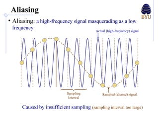
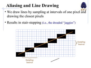
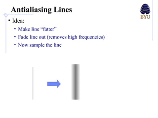
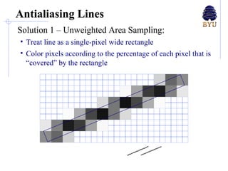
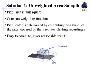
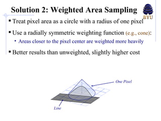
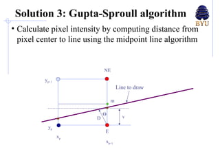
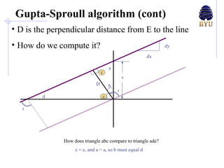
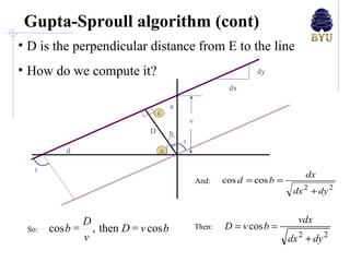
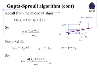
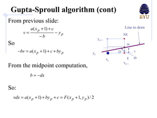
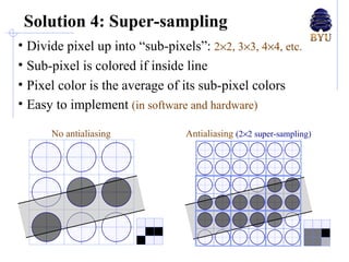
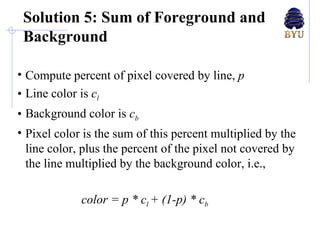
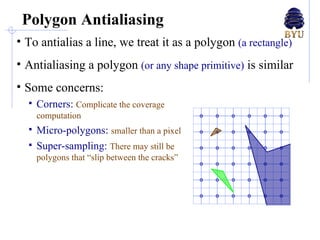
There are several techniques for antialiasing lines when rendering computer graphics to reduce jagged edges. These include making the line appear thicker by fading its edges, treating each pixel as a weighted area and calculating the percentage covered by the line, and dividing pixels into subpixels called super-sampling. More advanced methods compute the perpendicular distance from pixels to the line or determine pixel color as a blend of line and background colors based on the percentage coverage. These antialiasing methods aim to reduce aliasing caused by insufficient sampling of high-frequency signals.

1. CS 455 – Computer Graphics Antialiasing

2. Aliasing Aliasing: a high-frequency signal masquerading as a low frequency Caused by insufficient sampling (sampling interval too large) Sampling Interval Actual (high-frequency) signal Sampled (aliased) signal

3. Strobe light on dripping water: Temporal aliasing Spokes on a rotating wheel: Temporal aliasing Moir é patterns: Spatial aliasing Examples of Aliasing

4. Aliasing and Line Drawing We draw lines by sampling at intervals of one pixel and drawing the closest pixels Sampling Interval Sampling Interval Results in stair-stepping (i.e., the dreaded “jaggies”)

5. Antialiasing Lines Idea: Make line “fatter” Fade line out (removes high frequencies) Now sample the line

6. Antialiasing Lines Solution 1 – Unweighted Area Sampling: Treat line as a single-pixel wide rectangle Color pixels according to the percentage of each pixel that is “covered” by the rectangle

7. Solution 1: Unweighted Area Sampling Pixel area is unit square Constant weighting function Pixel color is determined by computing the amount of the pixel covered by the line, then shading accordingly Easy to compute, gives reasonable results Line One Pixel

8. Solution 2: Weighted Area Sampling Treat pixel area as a circle with a radius of one pixel Use a radially symmetric weighting function (e.g., cone) : Areas closer to the pixel center are weighted more heavily Better results than unweighted, slightly higher cost Line One Pixel

9. Solution 3: Gupta-Sproull algorithm Calculate pixel intensity by computing distance from pixel center to line using the midpoint line algorithm x p NE m E x p+1 Line to draw v y p y p+1  D

10. Gupta-Sproull algorithm (cont) D is the perpendicular distance from E to the line How do we compute it? a How does triangle abc compare to triangle ade? D c = e, and a = a, so b must equal d b c d e dx dy v r r

11. Gupta-Sproull algorithm (cont) D is the perpendicular distance from E to the line How do we compute it? a So: D b c d e dx dy v r r And: Then:

12. Gupta-Sproull algorithm (cont) Recall from the midpoint algorithm: So For pixel E: So: x p NE m E x p+1 Line to draw v y p y p +1  D

13. Gupta-Sproull algorithm (cont) From previous slide: So From the midpoint computation, So: x p NE m E x p+1 Line to draw v y p y p+1  D

14. Gupta-Sproull algorithm (cont) From the midpoint algorithm, we had the decision variable (remember?) Going back to our previous equation: x p NE m E x p+1 Line to draw v y p y p +1  D

15. Gupta-Sproull algorithm (cont) So, And the denominator is constant Since we are blurring the line, we also need to compute the distances to points y p – 1 and y p + 1

16. Gupta-Sproull algorithm (cont) If the NE pixel had been chosen:

17. Gupta-Sproull algorithm (cont) Compute midpoint line algorithm, with the following alterations: At each iteration of the algorithm: If the E pixel is chosen, set numerator = d + dx If the NE pixel is chosen, set numerator = d – dx Update d as in the regular algorithm Compute D = numerator/denominator Color the current pixel according to D Compute D upper = (2dx-2vdx)/denominator Compute D lower = (2dx+2vdx)/denominator Color upper and lower accordingly

18. Solution 4: Super-sampling Divide pixel up into “sub-pixels”: 2  2, 3  3, 4  4, etc. Sub-pixel is colored if inside line Pixel color is the average of its sub-pixel colors Easy to implement (in software and hardware) No antialiasing Antialiasing (2  2 super-sampling)

19. Solution 5: Sum of Foreground and Background Compute percent of pixel covered by line, p Line color is c l Background color is c b Pixel color is the sum of this percent multiplied by the line color, plus the percent of the pixel not covered by the line multiplied by the background color, i.e., color = p * c l + (1-p) * c b

20. Polygon Antialiasing To antialias a line, we treat it as a polygon (a rectangle) Antialiasing a polygon (or any shape primitive) is similar Some concerns: Corners: Complicate the coverage computation Micro-polygons: smaller than a pixel Super-sampling: There may still be polygons that “slip between the cracks”