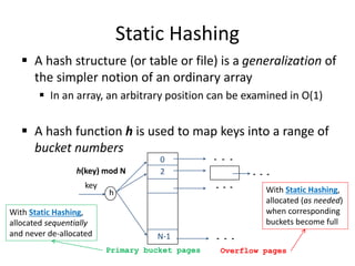
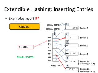
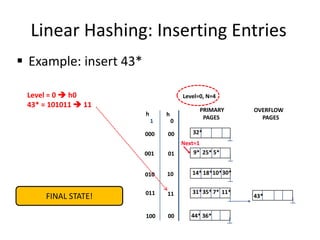
Database Applications (15-415)
DBMS Internals- Part V
Lecture 14, Oct 18, 2016
Mohammad Hammoud
Today…
 Last Session:
 DBMS Internals- Part IV
 Tree-based (i.e., B+ Tree– cont’d)
 Today’s Session:
 DBMS Internals- Part V
 Hash-based indexes and External Sorting
 Announcements:
 Mid-semester grades are out
 PS3 is out. It is due on Nov 1st
 Project 2 is due on Oct 27
DBMS Layers
Query Optimization
and Execution
Relational Operators
Files and Access Methods
Buffer Management
Disk Space Management
DB
Queries
Transaction
Manager
Lock
Manager
Recovery
Manager
Continue…
Outline
B+ Trees with Duplicates
B+ Trees with Key Compression
Bulk Loading of a B+ Tree
A Primer on Hash-Based Indexing
Static Hashing
Extendible Hashing

Hash-Based Indexing
 What indexing technique can we use to support range
searches (e.g., “Find s_name where gpa >= 3.0)?
 Tree-Based Indexing
 What about equality selections (e.g., “Find s_name
where sid = 102”?
 Tree-Based Indexing
 Hash-Based Indexing (cannot support range searches!)
 Hash-based indexing, however, proves to be very useful
in implementing relational operators (e.g., joins)
Outline
B+ Trees with Duplicates
B+ Trees with Key Compression
Bulk Loading of a B+ Tree
A Primer on Hash-Based Indexing
Static Hashing
Extendible Hashing

Static Hashing
 A hash structure (or table or file) is a generalization of
the simpler notion of an ordinary array
 In an array, an arbitrary position can be examined in O(1)
 A hash function h is used to map keys into a range of
bucket numbers
h(key) mod N
h
key
Primary bucket pages Overflow pages
2
0
N-1
With Static Hashing,
allocated sequentially
and never de-allocated
With Static Hashing,
allocated (as needed)
when corresponding
buckets become full
Static Hashing
 Data entries can be any of the three alternatives (A (1), A
(2) or A (3)- see previous lecture)
 Data entries can be sorted in buckets to speed up searches
 The hash function h is used to identify the bucket to which
a given key belongs and subsequently insert, delete or
locate a respective data record
 A hash function of the form h(key) = (a * key + b) works well
in practice
 A search ideally requires 1 disk I/O, while an insertion or a
deletion necessitates 2 disk I/Os
Static Hashing: Some Issues
 Similar to ISAM, the number of buckets is fixed!
 Cannot deal with insertions and deletions gracefully
 Long overflow chains can develop easily and degrade
performance!
 Pages can be initially kept only 80% full
 Dynamic hashing techniques can be used to fix
the problem
 Extendible Hashing (EH)
 Liner Hashing (LH)
Outline
B+ Trees with Duplicates
B+ Trees with Key Compression
Bulk Loading of a B+ Tree
A Primer on Hash-Based Indexing
Static Hashing
Extendible Hashing

Directory of Pointers
 How else (as opposed to overflow pages) can we add a
data record to a full bucket in a static hash file?
 Reorganize the table (e.g., by doubling the number of
buckets and redistributing the entries across the new
set of buckets)
 But, reading and writing all pages is expensive!
 In contrast, we can use a directory of pointers to buckets
 Buckets number can be doubled by doubling just the
directory and splitting “only” the bucket that overflowed
 The trick lies on how the hash function can be adjusted!
Extendible Hashing
 Extendible Hashing uses a directory of pointers to buckets
 The result of applying a hash
function h is treated as a
binary number and
the last d bits are
interpreted as an
offset into the directory
 d is referred to as the global depth
of the hash file and is kept as part
of the header of the file
00
01
10
11
DIRECTORY
Bucket A
Bucket B
Bucket C
Bucket D
DATA PAGES
10*
1* 21*
4* 12* 32* 16*
15* 7* 19*
5*
2
GLOBAL DEPTH
Extendible Hashing: Searching for Entries
 To search for a data entry, apply a hash function h to the
key and take the last d bits of its binary representation to
get the bucket number
 Example: search for 5*
00
01
10
11
DIRECTORY
Bucket A
Bucket B
Bucket C
Bucket D
DATA PAGES
10*
1* 21*
4* 12* 32* 16*
15* 7* 19*
5*
5 = 101
2
Extendible Hashing: Inserting Entries
 An entry can be inserted as follows:
 Find the appropriate bucket (as in search)
 Split the bucket if full and redistribute contents
(including the new entry to be inserted) across
the old bucket and its “split image”
 Double the directory if necessary
 Insert the given entry
Extendible Hashing: Inserting Entries
 Find the appropriate bucket (as in search), split the bucket
if full, double the directory if necessary and insert the
given entry
 Example: insert 13*
13*
00
01
10
11
DIRECTORY
Bucket A
Bucket B
Bucket C
Bucket D
10*
1* 21*
4* 12* 32* 16*
15* 7* 19*
5*
13 = 1101
2
Extendible Hashing: Inserting Entries
 Find the appropriate bucket (as in search), split the bucket
if full, double the directory if necessary and insert the
given entry
 Example: insert 20*
13*
00
01
10
11
DIRECTORY
Bucket A
Bucket B
Bucket C
Bucket D
10*
1* 21*
4* 12* 32* 16*
15* 7* 19*
5*
20 = 10100
FULL, hence, split and redistribute!
2
Extendible Hashing: Inserting Entries
 Find the appropriate bucket (as in search), split the bucket
if full, double the directory if necessary and insert the
given entry
 Example: insert 20*
13*
00
01
10
11
DIRECTORY
Bucket A
Bucket B
Bucket C
Bucket D
10*
1* 21*
32* 16*
15* 7* 19*
5*
20 = 10100
20* Bucket A2
(`split image'
of Bucket A)
4* 12*
2
Is this enough?
Extendible Hashing: Inserting Entries
 Find the appropriate bucket (as in search), split the bucket
if full, double the directory if necessary and insert the
given entry
 Example: insert 20*
13*
00
01
10
11
DIRECTORY
Bucket A
Bucket B
Bucket C
Bucket D
10*
1* 21*
32* 16*
15* 7* 19*
5*
20* Bucket A2
(`split image'
of Bucket A)
4* 12*
2
Double the directory and
increase the global depth
20 = 10100
Extendible Hashing: Inserting Entries
 Find the appropriate bucket (as in search), split the bucket
if full, double the directory if necessary and insert the
given entry
 Example: insert 20*
19*
0 00
001
010
011
1 00
101
110
111
3
DIRECTORY
Bucket A
Bucket B
Bucket C
Bucket D
Bucket A2
(`split image'
of Bucket A)
32*
1* 5* 21*13*
16*
10*
15* 7*
4* 20*
12*
GLOBAL DEPTH
These two bits indicate a data entry that
belongs to one of these two buckets
The third bit distinguishes between these
two buckets!
But, is it necessary always to
double the directory?
Extendible Hashing: Inserting Entries
 Find the appropriate bucket (as in search), split the bucket
if full, double the directory if necessary and insert the
given entry
 Example: insert 9*
9 = 1001
19*
000
001
010
011
100
101
110
111
3
DIRECTORY
Bucket A
Bucket B
Bucket C
Bucket D
Bucket A2
(`split image'
of Bucket A)
32*
1* 5* 21*13*
16*
10*
15* 7*
4* 20*
12*
GLOBAL DEPTH
FULL, hence, split!
Extendible Hashing: Inserting Entries
 Find the appropriate bucket (as in search), split the bucket
if full, double the directory if necessary and insert the
given entry
 Example: insert 9*
19*
000
001
010
011
100
101
110
111
3
DIRECTORY
Bucket A
Bucket B
Bucket C
Bucket D
Bucket A2
(`split image‘ of A)
32*
1*
16*
10*
15* 7*
4* 20*
12*
GLOBAL DEPTH
Bucket B2
(`split image‘ of B)
5* 21*13*
9*
Almost there…
9 = 1001
Extendible Hashing: Inserting Entries
 Find the appropriate bucket (as in search), split the bucket
if full, double the directory if necessary and insert the
given entry
 Example: insert 9*
19*
000
001
010
011
100
101
110
111
3
DIRECTORY
Bucket A
Bucket B
Bucket C
Bucket D
Bucket A2
(`split image‘ of A)
32*
1*
16*
10*
15* 7*
4* 20*
12*
GLOBAL DEPTH
Bucket A2
(`split image‘ of A)
5* 21*13*
9*
There was no need to
double the directory!
When NOT to double the
directory?
9 = 1001
Extendible Hashing: Inserting Entries
 Find the appropriate bucket (as in search), split the bucket
if full, double the directory if necessary and insert the
given entry
 Example: insert 9*
19*
000
001
010
011
100
101
110
111
3
DIRECTORY
Bucket A
Bucket B
Bucket C
Bucket D
Bucket A2
(`split image‘ of A)
32*
1*
16*
10*
15* 7*
4* 20*
12*
GLOBAL DEPTH
Bucket A2
(`split image‘ of A)
5* 21*13*
9*
If a bucket whose local depth
equals to the global depth is
split, the directory must be
doubled
3
2
2
3
3
LOCAL DEPTH
3
9 = 1001
Extendible Hashing: Inserting Entries
 Example: insert 9*
9 = 1001
19*
000
001
010
011
100
101
110
111
3
DIRECTORY
Bucket A
Bucket B
Bucket C
Bucket D
Bucket A2
(`split image'
of Bucket A)
32*
1* 5* 21*13*
16*
10*
15* 7*
4* 20*
12*
GLOBAL DEPTH
FULL, hence, split!
2
2
2
3
3
Repeat…
Because the local depth
(i.e., 2) is less than the
global depth (i.e., 3), NO
need to double the
directory
LOCAL DEPTH
Extendible Hashing: Inserting Entries
 Example: insert 9*
19*
000
001
010
011
100
101
110
111
3
DIRECTORY
Bucket A
Bucket B
Bucket C
Bucket D
Bucket A2
(`split image‘ of A)
32*
1*
16*
10*
15* 7*
4* 20*
12*
GLOBAL DEPTH
Bucket B2
(`split image‘ of B)
5* 21*13*
9*
3
2
2
3
3
LOCAL DEPTH
3
9 = 1001
Repeat…
Extendible Hashing: Inserting Entries
 Example: insert 9*
19*
000
001
010
011
100
101
110
111
3
DIRECTORY
Bucket A
Bucket B
Bucket C
Bucket D
Bucket A2
(`split image‘ of A)
32*
1*
16*
10*
15* 7*
4* 20*
12*
GLOBAL DEPTH
Bucket B2
(`split image‘ of B)
5* 21*13*
9*
3
2
2
3
3
LOCAL DEPTH
3
FINAL STATE!
9 = 1001
Repeat…
Extendible Hashing: Inserting Entries
 Example: insert 20*
Because the local depth
and the global depth are
both 2, we should double
the directory!
20 = 10100
13*
00
01
10
11
2
2
2
2
2
LOCAL DEPTH
GLOBAL DEPTH
DIRECTORY
Bucket A
Bucket B
Bucket C
Bucket D
DATA PAGES
10*
1* 21*
4* 12* 32* 16*
15* 7* 19*
5*
FULL, hence, split!
Repeat…
Extendible Hashing: Inserting Entries
 Example: insert 20*
Is this enough?
20*
00
01
10
11
2 2
2
2
LOCAL DEPTH 2
2
DIRECTORY
GLOBAL DEPTH
Bucket A
Bucket B
Bucket C
Bucket D
Bucket A2
(`split image'
of Bucket A)
1* 5* 21*13*
32*16*
10*
15* 7* 19*
4* 12*
Repeat…
20 = 10100
Extendible Hashing: Inserting Entries
 Example: insert 20*
19*
2
2
2
000
001
010
011
100
101
110
111
3
2
2
DIRECTORY
Bucket A
Bucket B
Bucket C
Bucket D
Bucket A2
(`split image'
of Bucket A)
32*
1* 5* 21*13*
16*
10*
15* 7*
4* 20*
12*
LOCAL DEPTH
GLOBAL DEPTH
Repeat…
Is this enough?
Extendible Hashing: Inserting Entries
 Example: insert 20*
19*
2
2
2
000
001
010
011
100
101
110
111
3
3
3
DIRECTORY
Bucket A
Bucket B
Bucket C
Bucket D
Bucket A2
(`split image'
of Bucket A)
32*
1* 5* 21*13*
16*
10*
15* 7*
4* 20*
12*
LOCAL DEPTH
GLOBAL DEPTH
Repeat…
FINAL STATE!
Outline
Linear Hashing
Why Sorting?
In-Memory vs. External Sorting
A Simple 2-Way External Merge Sorting
General External Merge Sorting
Optimizations: Replacement Sorting, Blocked I/O and Double Buffering

Linear Hashing
 Another way of adapting gracefully to insertions and
deletions (i.e., pursuing dynamic hashing) is to use
Linear Hashing (LH)
 In contrast to Extendible Hashing, LH
 Does not require a directory
 Deals naturally with collisions
 Offers a lot of flexibility w.r.t the timing of bucket split
(allowing trading off greater overflow chains for higher
average space utilization)
How Linear Hashing Works?
 LH uses a family of hash functions h0, h1, h2, ...
 hi(key) = h(key) mod(2iN); N = initial # buckets
 h is some hash function (range is not 0 to N-1)
 If N = 2d0, for some d0, hi consists of applying h and
looking at the last di bits, where di = d0 + i
 hi+1 doubles the range of hi (similar to directory
doubling)
How Linear Hashing Works? (Cont’d)
 LH uses overflow pages, and chooses buckets to split in
a round-robin fashion
 Splitting proceeds in “rounds”
 A round ends when all NR
(for round R) initial
buckets are split
 Buckets 0 to Next-1
have been split;
Next to NR yet to be split
 Current round number
is referred to as Level
Level
h
Buckets that existed at the
beginning of this round:
this is the range of
Next
Buckets split
in this round
‘split image’
buckets created
in this round
Linear Hashing: Searching For Entries
 To find a bucket for data entry r, find hLevel(r):
 If hLevel(r) in range `Next to NR’, r belongs there
 Else, r could belong to bucket hLevel(r) or bucket
hLevel(r) + NR; must apply hLevel+1(r) to find out
 Example: search for 5* 0
h
h
1
00
01
10
11
000
001
010
011
Next=0
PRIMARY
PAGES
Data entry r
with h(r)=5
Primary
bucket page
44* 36*
32*
25*
9* 5*
14* 18*10*30*
31*35* 11*
7*
Level=0, N=4
Level = 0  h0
5* = 101  01
Linear Hashing: Inserting Entries
 Find bucket as in search
 If the bucket to insert the data entry into is full:
 Add an overflow page and insert data entry
 (Maybe) Split Next bucket and increment Next
 Some points to Keep in mind:
 Unlike Extendible Hashing, when an insert triggers a split, the
bucket into which the data entry is inserted is not necessarily
the bucket that is split
 As in Static Hashing, an overflow page is added to store the
newly inserted data entry
 However, since the bucket to split is chosen in a round-robin
fashion, eventually all buckets will be split
Linear Hashing: Inserting Entries
 Example: insert 43*
0
h
h
1
Level=0, N=4
00
01
10
11
000
001
010
011
Next=0
PRIMARY
PAGES
44* 36*
32*
25*
9* 5*
14* 18*10*30*
31*35* 11*
7*
Level = 0  h0
43* = 101011  11
Add an overflow page and
insert data entry
Linear Hashing: Inserting Entries
 Example: insert 43*
0
h
h
1
Level=0, N=4
00
01
10
11
000
001
010
011
Next=0
PRIMARY
PAGES
44* 36*
32*
25*
9* 5*
14* 18*10*30*
31*35* 11*
7*
Level = 0  h0
43* = 101011  11
43*
OVERFLOW
PAGES
Split Next bucket and
increment Next
Linear Hashing: Inserting Entries
 Example: insert 43*
Level=0, N=4
Next=0
PRIMARY
PAGES
32*
25*
9* 5*
14* 18*10*30*
31*35* 11*
7*
Level = 0  h0
43* = 101011  11
43*
OVERFLOW
PAGES
44* 36*
Almost there…
0
h
h
1
00
01
10
11
000
001
010
011
00
100
Linear Hashing: Inserting Entries
 Example: insert 43*
Level=0, N=4
Next=1
PRIMARY
PAGES
32*
25*
9* 5*
14* 18*10*30*
31*35* 11*
7*
Level = 0  h0
43* = 101011  11
43*
OVERFLOW
PAGES
44* 36*
FINAL STATE!
0
h
h
1
00
01
10
11
000
001
010
011
00
100
Linear Hashing: Inserting Entries
 Another Example: insert 50*
Level = 0  h0
50* = 110010  10
Add an overflow page and
insert data entry
0
h
h1
22*
00
01
10
11
000
001
010
011
00
100
Next=3
01
10
101
110
Level=0, N= 4
PRIMARY
PAGES
OVERFLOW
PAGES
32*
9*
5*
14*
25*
66* 10*
18* 34*
35*
31* 7* 11* 43*
44*36*
37*29*
30*
Linear Hashing: Inserting Entries
 Another Example: insert 50*
Level = 0  h0
50* = 110010  10
0
h
h1
22*
00
01
10
11
000
001
010
011
00
100
Next=3
01
10
101
110
PRIMARY
PAGES
OVERFLOW
PAGES
32*
9*
5*
14*
25*
66* 10*
18* 34*
35*
31* 7* 11* 43*
44*36*
37*29*
30*
50*
Split Next bucket and
increment Next
Level=0, N= 4
Linear Hashing: Inserting Entries
 Another Example: insert 50*
Level = 0  h0
50* = 110010  10
Almost there…
0
h
h1
37*
00
01
10
11
000
001
010
011
00
100
10
101
110
111
11
PRIMARY
PAGES
OVERFLOW
PAGES
11
32*
9* 25*
66* 18* 10* 34*
35* 11*
44* 36*
5* 29*
43*
14* 30* 22*
31*7*
50*
Level=0
Next=3
Linear Hashing: Inserting Entries
 Another Example: insert 50*
Level = 0  h0
50* = 110010  10
Almost there…
0
h
h1
37*
00
01
10
11
000
001
010
011
00
100
10
101
110
Next=0
111
11
PRIMARY
PAGES
OVERFLOW
PAGES
11
32*
9* 25*
66* 18* 10* 34*
35* 11*
44* 36*
5* 29*
43*
14* 30* 22*
31*7*
50*
Level=0
Linear Hashing: Inserting Entries
 Another Example: insert 50*
Level = 0  h0
50* = 110010  10
FINAL STATE!
0
h
h1
37*
00
01
10
11
000
001
010
011
00
100
10
101
110
Next=0
111
11
PRIMARY
PAGES
OVERFLOW
PAGES
11
32*
9* 25*
66* 18* 10* 34*
35* 11*
44* 36*
5* 29*
43*
14* 30* 22*
31*7*
50*
Level=1
Linear Hashing: Deleting Entries
 Deletion is essentially the inverse of insertion
 If the last bucket in the file is empty, it can be removed and
Next can be decremented
 If Next is zero and the last bucket becomes empty
 Next is made to point to bucket M/2 -1 (where M is the current
number of buckets)
 Level is decremented
 The empty bucket is removed
 The insertion examples can be worked out backwards as
examples of deletions!
DBMS Layers
Query Optimization
and Execution
Relational Operators
Files and Access Methods
Buffer Management
Disk Space Management
DB
Queries
Transaction
Manager
Lock
Manager
Recovery
Manager
But, before we will
discuss “Sorting”
Outline
Linear Hashing
Why Sorting?
In-Memory vs. External Sorting
A Simple 2-Way External Merge Sorting
General External Merge Sorting
Optimizations: Replacement Sorting, Blocked I/O and Double Buffering

When Does A DBMS Sort Data?
 Users may want answers in some order
 SELECT FROM student ORDER BY name
 SELECT S.rating, MIN (S.age) FROM Sailors S GROUP BY S.rating
 Bulk loading a B+ tree index involves sorting
 Sorting is useful in eliminating duplicates records
 The Sort-Merge Join algorithm involves sorting
(next session!)
Outline
Linear Hashing
Why Sorting?
In-Memory vs. External Sorting
A Simple 2-Way External Merge Sorting
General External Merge Sorting
Optimizations: Replacement Sorting, Blocked I/O and Double Buffering

In-Memory vs. External Sorting
 Assume we want to sort 60GB of data on a machine
with only 8GB of RAM
 In-Memory Sort (e.g., Quicksort) ?
 Yes, but data do not fit in memory
 What about relying on virtual memory?
 In this case, external sorting is needed
 In-memory sorting is orthogonal to external sorting!
Outline
Linear Hashing
Why Sorting?
In-Memory vs. External Sorting
A Simple 2-Way External Merge Sorting
General External Merge Sorting
Optimizations: Replacement Sorting, Blocked I/O and Double Buffering

A Simple Two-Way Merge Sort
 IDEA: Sort sub-files that can fit in memory and merge
 Let us refer to each sorted sub-file as a run
 Algorithm:
 Pass 1: Read a page into memory, sort it, write it
 1-page runs are produced
 Passes 2, 3, etc.,: Merge pairs (hence, 2-way) of runs
to produce longer runs until only one run is left
A Simple Two-Way Merge Sort
 Algorithm:
 Pass 1: Read a page into memory, sort it, write it
 How many buffer pages are needed?
 Passes 2, 3, etc.,: Merge pairs (hence, 2-way) of runs to
produce longer runs until only one run is left
 How many buffer pages are needed?
Main memory buffers
INPUT 1
INPUT 2
OUTPUT
Disk
Disk
ONE
THREE
2-Way Merge Sort: An Example
Input File
1-Page Runs
2-Page Runs
4-Page Runs
8-Page Runs
PASS 0
PASS 1
PASS 2
PASS 3
9
3,4 6,2 9,4 8,7 5,6 3,1 2
3,4 5,6
2,6 4,9 7,8 1,3 2
2,3
4,6
4,7
8,9
1,3
5,6 2
2,3
4,4
6,7
8,9
1,2
3,5
6
1,2
2,3
3,4
4,5
6,6
7,8
2-Way Merge Sort: I/O Cost Analysis
 If the number of pages in the input file is 2k
 How many runs are produced in pass 0 and of what size?
 2k 1-page runs
 How many runs are produced in pass 1 and of what size?
 2k-1 2-page runs
 How many runs are produced in pass 2 and of what size?
 2k-2 4-page runs
 How many runs are produced in pass k and of what size?
 2k-k 2k-page runs (or 1 run of size 2k)
 For N number of pages, how many passes are incurred?

 How many pages do we read and write in each pass?
 2N
 What is the overall cost?

  1
log2 
N
  )
1
log
(
2 2 
 N
N
2-Way Merge Sort: An Example
Input File
1-Page Runs
2-Page Runs
4-Page Runs
8-Page Runs
PASS 0
PASS 1
PASS 2
PASS 3
9
3,4 6,2 9,4 8,7 5,6 3,1 2
3,4 5,6
2,6 4,9 7,8 1,3 2
2,3
4,6
4,7
8,9
1,3
5,6 2
2,3
4,4
6,7
8,9
1,2
3,5
6
1,2
2,3
3,4
4,5
6,6
7,8
Formula Check:
= (2 × 8) × (3 + 1) = 64 I/Os
Correct!
  )
1
log
(
2 2 
 N
N
  1
8
log2 
= 4 passes
Outline
Linear Hashing
Why Sorting?
In-Memory vs. External Sorting
A Simple 2-Way External Merge Sorting
General External Merge Sorting
Optimizations: Replacement Sorting, Blocked I/O and Double Buffering

B-Way Merge Sort
 How can we sort a file with N pages using B buffer pages?
 Pass 0: use B buffer pages and sort internally
 This will produce sorted B-page runs
 Passes 1, 2, …: use B – 1 buffer pages for input and the
remaining page for output; do (B-1)-way merge in each run
 
N B
/
B Main memory buffers
INPUT 1
INPUT B-1
OUTPUT
Disk
Disk
INPUT 2
. . . . . .
. . .
B-Way Merge Sort: I/O Cost Analysis
 I/O cost = 2N × Number of passes
 Number of passes =
 Assume the previous example (i.e., 8 pages), but using
5 buffer pages (instead of 2)
 I/O cost = 32 (as opposed to 64)
 Therefore, increasing the number of buffer pages
minimizes the number of passes and accordingly the
I/O cost!
 
 
1 1
 
log /
B N B
Number of Passes of B-Way Sort
N B=3 B=5 B=9 B=17 B=129 B=257
100 7 4 3 2 1 1
1,000 10 5 4 3 2 2
10,000 13 7 5 4 2 2
100,000 17 9 6 5 3 3
1,000,000 20 10 7 5 3 3
10,000,000 23 12 8 6 4 3
100,000,000 26 14 9 7 4 4
1,000,000,000 30 15 10 8 5 4
High Fan-in during merging is crucial!
How else can we minimize I/O cost?
Outline
Linear Hashing
Why Sorting?
In-Memory vs. External Sorting
A Simple 2-Way External Merge Sorting
General External Merge Sorting
Optimizations: Replacement Sorting, Blocked I/O and Double Buffering

Replacement Sort
 With a more aggressive implementation of B-way sort,
we can write out runs of 2×B (on average) internally
sorted pages
 This is referred to as replacement sort
12
4
INPUT
8
10
CURRENT SET
2
3
5
OUTPUT
IDEA: Pick the tuple in the current set with the smallest value that is greater than
the largest value in the output buffer and append it to the output buffer
Replacement Sort
 With a more aggressive implementation of B-way sort,
we can write out runs of 2×B (on average) internally
sorted pages
 This is referred to as replacement sort
12
4
INPUT
8
10
CURRENT SET
2
3
5
OUTPUT
When do we terminate the current run and start a new one?
Blocked I/O and Double Buffering
 So far, we assumed random disk accesses
 Would cost change if we assume that reads and writes
are done sequentially?
 Yes
 How can we incorporate this fact into our
cost model?
 Use bigger units (this is referred to as Blocked I/O)
 Mask I/O delays through pre-fetching (this is
referred to as double buffering)
Blocked I/O
 Normally, we go with‘B’ buffers of size (say) 1 page
INPUT 1
INPUT 5
OUTPUT
Disk
Disk
INPUT 2
. . . . . .
. . .
Blocked I/O
 Normally, we go with‘B’ buffers of size (say) 1 page
 INSTEAD: let us go with B/b buffers, of size ‘b’ pages
3 Main memory buffers
INPUT 1
INPUT 2
OUTPUT
Disk
Disk
. . .
. . .
Blocked I/O
 Normally, we go with‘B’ buffers of size (say) 1 page
 INSTEAD: let us go with B/b buffers, of size ‘b’ pages
 What is the main advantage?
 Fewer random accesses (as some of the pages will be
arranged sequentially!)
 What is the main disadvantage?
 Smaller fan-in and accordingly larger number of passes!
Double Buffering
 Normally, when, say ‘INPUT1’ is exhausted
 We issue a ‘read’ request and
 We wait …
B Main memory buffers
INPUT 1
INPUT B-1
OUTPUT
Disk
Disk
INPUT 2
. . . . . .
. . .
Double Buffering
 INSTEAD: pre-fetch INPUT1’ into a `shadow block’
 When INPUT1 is exhausted, issue a ‘read’
 BUT, also proceed with INPUT1’
 Thus, the CPU can never go idle!
OUTPUT
OUTPUT'
Disk Disk
INPUT 1
INPUT k
INPUT 2
INPUT 1'
INPUT 2'
INPUT k'
block size
b
B main memory buffers, k-way merge
Next Class
Query Optimization
and Execution
Relational Operators
Files and Access Methods
Buffer Management
Disk Space Management
DB
Queries
Transaction
Manager
Lock
Manager
Recovery
Manager
Continue…

Lecture14-Hash-Based-Indexing-and-Sorting-MHH-18Oct-2016.pptx

  • 1.
    Database Applications (15-415) DBMSInternals- Part V Lecture 14, Oct 18, 2016 Mohammad Hammoud
  • 2.
    Today…  Last Session: DBMS Internals- Part IV  Tree-based (i.e., B+ Tree– cont’d)  Today’s Session:  DBMS Internals- Part V  Hash-based indexes and External Sorting  Announcements:  Mid-semester grades are out  PS3 is out. It is due on Nov 1st  Project 2 is due on Oct 27
  • 3.
    DBMS Layers Query Optimization andExecution Relational Operators Files and Access Methods Buffer Management Disk Space Management DB Queries Transaction Manager Lock Manager Recovery Manager Continue…
  • 4.
    Outline B+ Trees withDuplicates B+ Trees with Key Compression Bulk Loading of a B+ Tree A Primer on Hash-Based Indexing Static Hashing Extendible Hashing 
  • 5.
    Hash-Based Indexing  Whatindexing technique can we use to support range searches (e.g., “Find s_name where gpa >= 3.0)?  Tree-Based Indexing  What about equality selections (e.g., “Find s_name where sid = 102”?  Tree-Based Indexing  Hash-Based Indexing (cannot support range searches!)  Hash-based indexing, however, proves to be very useful in implementing relational operators (e.g., joins)
  • 6.
    Outline B+ Trees withDuplicates B+ Trees with Key Compression Bulk Loading of a B+ Tree A Primer on Hash-Based Indexing Static Hashing Extendible Hashing 
  • 7.
    Static Hashing  Ahash structure (or table or file) is a generalization of the simpler notion of an ordinary array  In an array, an arbitrary position can be examined in O(1)  A hash function h is used to map keys into a range of bucket numbers h(key) mod N h key Primary bucket pages Overflow pages 2 0 N-1 With Static Hashing, allocated sequentially and never de-allocated With Static Hashing, allocated (as needed) when corresponding buckets become full
  • 8.
    Static Hashing  Dataentries can be any of the three alternatives (A (1), A (2) or A (3)- see previous lecture)  Data entries can be sorted in buckets to speed up searches  The hash function h is used to identify the bucket to which a given key belongs and subsequently insert, delete or locate a respective data record  A hash function of the form h(key) = (a * key + b) works well in practice  A search ideally requires 1 disk I/O, while an insertion or a deletion necessitates 2 disk I/Os
  • 9.
    Static Hashing: SomeIssues  Similar to ISAM, the number of buckets is fixed!  Cannot deal with insertions and deletions gracefully  Long overflow chains can develop easily and degrade performance!  Pages can be initially kept only 80% full  Dynamic hashing techniques can be used to fix the problem  Extendible Hashing (EH)  Liner Hashing (LH)
  • 10.
    Outline B+ Trees withDuplicates B+ Trees with Key Compression Bulk Loading of a B+ Tree A Primer on Hash-Based Indexing Static Hashing Extendible Hashing 
  • 11.
    Directory of Pointers How else (as opposed to overflow pages) can we add a data record to a full bucket in a static hash file?  Reorganize the table (e.g., by doubling the number of buckets and redistributing the entries across the new set of buckets)  But, reading and writing all pages is expensive!  In contrast, we can use a directory of pointers to buckets  Buckets number can be doubled by doubling just the directory and splitting “only” the bucket that overflowed  The trick lies on how the hash function can be adjusted!
  • 12.
    Extendible Hashing  ExtendibleHashing uses a directory of pointers to buckets  The result of applying a hash function h is treated as a binary number and the last d bits are interpreted as an offset into the directory  d is referred to as the global depth of the hash file and is kept as part of the header of the file 00 01 10 11 DIRECTORY Bucket A Bucket B Bucket C Bucket D DATA PAGES 10* 1* 21* 4* 12* 32* 16* 15* 7* 19* 5* 2 GLOBAL DEPTH
  • 13.
    Extendible Hashing: Searchingfor Entries  To search for a data entry, apply a hash function h to the key and take the last d bits of its binary representation to get the bucket number  Example: search for 5* 00 01 10 11 DIRECTORY Bucket A Bucket B Bucket C Bucket D DATA PAGES 10* 1* 21* 4* 12* 32* 16* 15* 7* 19* 5* 5 = 101 2
  • 14.
    Extendible Hashing: InsertingEntries  An entry can be inserted as follows:  Find the appropriate bucket (as in search)  Split the bucket if full and redistribute contents (including the new entry to be inserted) across the old bucket and its “split image”  Double the directory if necessary  Insert the given entry
  • 15.
    Extendible Hashing: InsertingEntries  Find the appropriate bucket (as in search), split the bucket if full, double the directory if necessary and insert the given entry  Example: insert 13* 13* 00 01 10 11 DIRECTORY Bucket A Bucket B Bucket C Bucket D 10* 1* 21* 4* 12* 32* 16* 15* 7* 19* 5* 13 = 1101 2
  • 16.
    Extendible Hashing: InsertingEntries  Find the appropriate bucket (as in search), split the bucket if full, double the directory if necessary and insert the given entry  Example: insert 20* 13* 00 01 10 11 DIRECTORY Bucket A Bucket B Bucket C Bucket D 10* 1* 21* 4* 12* 32* 16* 15* 7* 19* 5* 20 = 10100 FULL, hence, split and redistribute! 2
  • 17.
    Extendible Hashing: InsertingEntries  Find the appropriate bucket (as in search), split the bucket if full, double the directory if necessary and insert the given entry  Example: insert 20* 13* 00 01 10 11 DIRECTORY Bucket A Bucket B Bucket C Bucket D 10* 1* 21* 32* 16* 15* 7* 19* 5* 20 = 10100 20* Bucket A2 (`split image' of Bucket A) 4* 12* 2 Is this enough?
  • 18.
    Extendible Hashing: InsertingEntries  Find the appropriate bucket (as in search), split the bucket if full, double the directory if necessary and insert the given entry  Example: insert 20* 13* 00 01 10 11 DIRECTORY Bucket A Bucket B Bucket C Bucket D 10* 1* 21* 32* 16* 15* 7* 19* 5* 20* Bucket A2 (`split image' of Bucket A) 4* 12* 2 Double the directory and increase the global depth 20 = 10100
  • 19.
    Extendible Hashing: InsertingEntries  Find the appropriate bucket (as in search), split the bucket if full, double the directory if necessary and insert the given entry  Example: insert 20* 19* 0 00 001 010 011 1 00 101 110 111 3 DIRECTORY Bucket A Bucket B Bucket C Bucket D Bucket A2 (`split image' of Bucket A) 32* 1* 5* 21*13* 16* 10* 15* 7* 4* 20* 12* GLOBAL DEPTH These two bits indicate a data entry that belongs to one of these two buckets The third bit distinguishes between these two buckets! But, is it necessary always to double the directory?
  • 20.
    Extendible Hashing: InsertingEntries  Find the appropriate bucket (as in search), split the bucket if full, double the directory if necessary and insert the given entry  Example: insert 9* 9 = 1001 19* 000 001 010 011 100 101 110 111 3 DIRECTORY Bucket A Bucket B Bucket C Bucket D Bucket A2 (`split image' of Bucket A) 32* 1* 5* 21*13* 16* 10* 15* 7* 4* 20* 12* GLOBAL DEPTH FULL, hence, split!
  • 21.
    Extendible Hashing: InsertingEntries  Find the appropriate bucket (as in search), split the bucket if full, double the directory if necessary and insert the given entry  Example: insert 9* 19* 000 001 010 011 100 101 110 111 3 DIRECTORY Bucket A Bucket B Bucket C Bucket D Bucket A2 (`split image‘ of A) 32* 1* 16* 10* 15* 7* 4* 20* 12* GLOBAL DEPTH Bucket B2 (`split image‘ of B) 5* 21*13* 9* Almost there… 9 = 1001
  • 22.
    Extendible Hashing: InsertingEntries  Find the appropriate bucket (as in search), split the bucket if full, double the directory if necessary and insert the given entry  Example: insert 9* 19* 000 001 010 011 100 101 110 111 3 DIRECTORY Bucket A Bucket B Bucket C Bucket D Bucket A2 (`split image‘ of A) 32* 1* 16* 10* 15* 7* 4* 20* 12* GLOBAL DEPTH Bucket A2 (`split image‘ of A) 5* 21*13* 9* There was no need to double the directory! When NOT to double the directory? 9 = 1001
  • 23.
    Extendible Hashing: InsertingEntries  Find the appropriate bucket (as in search), split the bucket if full, double the directory if necessary and insert the given entry  Example: insert 9* 19* 000 001 010 011 100 101 110 111 3 DIRECTORY Bucket A Bucket B Bucket C Bucket D Bucket A2 (`split image‘ of A) 32* 1* 16* 10* 15* 7* 4* 20* 12* GLOBAL DEPTH Bucket A2 (`split image‘ of A) 5* 21*13* 9* If a bucket whose local depth equals to the global depth is split, the directory must be doubled 3 2 2 3 3 LOCAL DEPTH 3 9 = 1001
  • 24.
    Extendible Hashing: InsertingEntries  Example: insert 9* 9 = 1001 19* 000 001 010 011 100 101 110 111 3 DIRECTORY Bucket A Bucket B Bucket C Bucket D Bucket A2 (`split image' of Bucket A) 32* 1* 5* 21*13* 16* 10* 15* 7* 4* 20* 12* GLOBAL DEPTH FULL, hence, split! 2 2 2 3 3 Repeat… Because the local depth (i.e., 2) is less than the global depth (i.e., 3), NO need to double the directory LOCAL DEPTH
  • 25.
    Extendible Hashing: InsertingEntries  Example: insert 9* 19* 000 001 010 011 100 101 110 111 3 DIRECTORY Bucket A Bucket B Bucket C Bucket D Bucket A2 (`split image‘ of A) 32* 1* 16* 10* 15* 7* 4* 20* 12* GLOBAL DEPTH Bucket B2 (`split image‘ of B) 5* 21*13* 9* 3 2 2 3 3 LOCAL DEPTH 3 9 = 1001 Repeat…
  • 26.
    Extendible Hashing: InsertingEntries  Example: insert 9* 19* 000 001 010 011 100 101 110 111 3 DIRECTORY Bucket A Bucket B Bucket C Bucket D Bucket A2 (`split image‘ of A) 32* 1* 16* 10* 15* 7* 4* 20* 12* GLOBAL DEPTH Bucket B2 (`split image‘ of B) 5* 21*13* 9* 3 2 2 3 3 LOCAL DEPTH 3 FINAL STATE! 9 = 1001 Repeat…
  • 27.
    Extendible Hashing: InsertingEntries  Example: insert 20* Because the local depth and the global depth are both 2, we should double the directory! 20 = 10100 13* 00 01 10 11 2 2 2 2 2 LOCAL DEPTH GLOBAL DEPTH DIRECTORY Bucket A Bucket B Bucket C Bucket D DATA PAGES 10* 1* 21* 4* 12* 32* 16* 15* 7* 19* 5* FULL, hence, split! Repeat…
  • 28.
    Extendible Hashing: InsertingEntries  Example: insert 20* Is this enough? 20* 00 01 10 11 2 2 2 2 LOCAL DEPTH 2 2 DIRECTORY GLOBAL DEPTH Bucket A Bucket B Bucket C Bucket D Bucket A2 (`split image' of Bucket A) 1* 5* 21*13* 32*16* 10* 15* 7* 19* 4* 12* Repeat… 20 = 10100
  • 29.
    Extendible Hashing: InsertingEntries  Example: insert 20* 19* 2 2 2 000 001 010 011 100 101 110 111 3 2 2 DIRECTORY Bucket A Bucket B Bucket C Bucket D Bucket A2 (`split image' of Bucket A) 32* 1* 5* 21*13* 16* 10* 15* 7* 4* 20* 12* LOCAL DEPTH GLOBAL DEPTH Repeat… Is this enough?
  • 30.
    Extendible Hashing: InsertingEntries  Example: insert 20* 19* 2 2 2 000 001 010 011 100 101 110 111 3 3 3 DIRECTORY Bucket A Bucket B Bucket C Bucket D Bucket A2 (`split image' of Bucket A) 32* 1* 5* 21*13* 16* 10* 15* 7* 4* 20* 12* LOCAL DEPTH GLOBAL DEPTH Repeat… FINAL STATE!
  • 31.
    Outline Linear Hashing Why Sorting? In-Memoryvs. External Sorting A Simple 2-Way External Merge Sorting General External Merge Sorting Optimizations: Replacement Sorting, Blocked I/O and Double Buffering 
  • 32.
    Linear Hashing  Anotherway of adapting gracefully to insertions and deletions (i.e., pursuing dynamic hashing) is to use Linear Hashing (LH)  In contrast to Extendible Hashing, LH  Does not require a directory  Deals naturally with collisions  Offers a lot of flexibility w.r.t the timing of bucket split (allowing trading off greater overflow chains for higher average space utilization)
  • 33.
    How Linear HashingWorks?  LH uses a family of hash functions h0, h1, h2, ...  hi(key) = h(key) mod(2iN); N = initial # buckets  h is some hash function (range is not 0 to N-1)  If N = 2d0, for some d0, hi consists of applying h and looking at the last di bits, where di = d0 + i  hi+1 doubles the range of hi (similar to directory doubling)
  • 34.
    How Linear HashingWorks? (Cont’d)  LH uses overflow pages, and chooses buckets to split in a round-robin fashion  Splitting proceeds in “rounds”  A round ends when all NR (for round R) initial buckets are split  Buckets 0 to Next-1 have been split; Next to NR yet to be split  Current round number is referred to as Level Level h Buckets that existed at the beginning of this round: this is the range of Next Buckets split in this round ‘split image’ buckets created in this round
  • 35.
    Linear Hashing: SearchingFor Entries  To find a bucket for data entry r, find hLevel(r):  If hLevel(r) in range `Next to NR’, r belongs there  Else, r could belong to bucket hLevel(r) or bucket hLevel(r) + NR; must apply hLevel+1(r) to find out  Example: search for 5* 0 h h 1 00 01 10 11 000 001 010 011 Next=0 PRIMARY PAGES Data entry r with h(r)=5 Primary bucket page 44* 36* 32* 25* 9* 5* 14* 18*10*30* 31*35* 11* 7* Level=0, N=4 Level = 0  h0 5* = 101  01
  • 36.
    Linear Hashing: InsertingEntries  Find bucket as in search  If the bucket to insert the data entry into is full:  Add an overflow page and insert data entry  (Maybe) Split Next bucket and increment Next  Some points to Keep in mind:  Unlike Extendible Hashing, when an insert triggers a split, the bucket into which the data entry is inserted is not necessarily the bucket that is split  As in Static Hashing, an overflow page is added to store the newly inserted data entry  However, since the bucket to split is chosen in a round-robin fashion, eventually all buckets will be split
  • 37.
    Linear Hashing: InsertingEntries  Example: insert 43* 0 h h 1 Level=0, N=4 00 01 10 11 000 001 010 011 Next=0 PRIMARY PAGES 44* 36* 32* 25* 9* 5* 14* 18*10*30* 31*35* 11* 7* Level = 0  h0 43* = 101011  11 Add an overflow page and insert data entry
  • 38.
    Linear Hashing: InsertingEntries  Example: insert 43* 0 h h 1 Level=0, N=4 00 01 10 11 000 001 010 011 Next=0 PRIMARY PAGES 44* 36* 32* 25* 9* 5* 14* 18*10*30* 31*35* 11* 7* Level = 0  h0 43* = 101011  11 43* OVERFLOW PAGES Split Next bucket and increment Next
  • 39.
    Linear Hashing: InsertingEntries  Example: insert 43* Level=0, N=4 Next=0 PRIMARY PAGES 32* 25* 9* 5* 14* 18*10*30* 31*35* 11* 7* Level = 0  h0 43* = 101011  11 43* OVERFLOW PAGES 44* 36* Almost there… 0 h h 1 00 01 10 11 000 001 010 011 00 100
  • 40.
    Linear Hashing: InsertingEntries  Example: insert 43* Level=0, N=4 Next=1 PRIMARY PAGES 32* 25* 9* 5* 14* 18*10*30* 31*35* 11* 7* Level = 0  h0 43* = 101011  11 43* OVERFLOW PAGES 44* 36* FINAL STATE! 0 h h 1 00 01 10 11 000 001 010 011 00 100
  • 41.
    Linear Hashing: InsertingEntries  Another Example: insert 50* Level = 0  h0 50* = 110010  10 Add an overflow page and insert data entry 0 h h1 22* 00 01 10 11 000 001 010 011 00 100 Next=3 01 10 101 110 Level=0, N= 4 PRIMARY PAGES OVERFLOW PAGES 32* 9* 5* 14* 25* 66* 10* 18* 34* 35* 31* 7* 11* 43* 44*36* 37*29* 30*
  • 42.
    Linear Hashing: InsertingEntries  Another Example: insert 50* Level = 0  h0 50* = 110010  10 0 h h1 22* 00 01 10 11 000 001 010 011 00 100 Next=3 01 10 101 110 PRIMARY PAGES OVERFLOW PAGES 32* 9* 5* 14* 25* 66* 10* 18* 34* 35* 31* 7* 11* 43* 44*36* 37*29* 30* 50* Split Next bucket and increment Next Level=0, N= 4
  • 43.
    Linear Hashing: InsertingEntries  Another Example: insert 50* Level = 0  h0 50* = 110010  10 Almost there… 0 h h1 37* 00 01 10 11 000 001 010 011 00 100 10 101 110 111 11 PRIMARY PAGES OVERFLOW PAGES 11 32* 9* 25* 66* 18* 10* 34* 35* 11* 44* 36* 5* 29* 43* 14* 30* 22* 31*7* 50* Level=0 Next=3
  • 44.
    Linear Hashing: InsertingEntries  Another Example: insert 50* Level = 0  h0 50* = 110010  10 Almost there… 0 h h1 37* 00 01 10 11 000 001 010 011 00 100 10 101 110 Next=0 111 11 PRIMARY PAGES OVERFLOW PAGES 11 32* 9* 25* 66* 18* 10* 34* 35* 11* 44* 36* 5* 29* 43* 14* 30* 22* 31*7* 50* Level=0
  • 45.
    Linear Hashing: InsertingEntries  Another Example: insert 50* Level = 0  h0 50* = 110010  10 FINAL STATE! 0 h h1 37* 00 01 10 11 000 001 010 011 00 100 10 101 110 Next=0 111 11 PRIMARY PAGES OVERFLOW PAGES 11 32* 9* 25* 66* 18* 10* 34* 35* 11* 44* 36* 5* 29* 43* 14* 30* 22* 31*7* 50* Level=1
  • 46.
    Linear Hashing: DeletingEntries  Deletion is essentially the inverse of insertion  If the last bucket in the file is empty, it can be removed and Next can be decremented  If Next is zero and the last bucket becomes empty  Next is made to point to bucket M/2 -1 (where M is the current number of buckets)  Level is decremented  The empty bucket is removed  The insertion examples can be worked out backwards as examples of deletions!
  • 47.
    DBMS Layers Query Optimization andExecution Relational Operators Files and Access Methods Buffer Management Disk Space Management DB Queries Transaction Manager Lock Manager Recovery Manager But, before we will discuss “Sorting”
  • 48.
    Outline Linear Hashing Why Sorting? In-Memoryvs. External Sorting A Simple 2-Way External Merge Sorting General External Merge Sorting Optimizations: Replacement Sorting, Blocked I/O and Double Buffering 
  • 49.
    When Does ADBMS Sort Data?  Users may want answers in some order  SELECT FROM student ORDER BY name  SELECT S.rating, MIN (S.age) FROM Sailors S GROUP BY S.rating  Bulk loading a B+ tree index involves sorting  Sorting is useful in eliminating duplicates records  The Sort-Merge Join algorithm involves sorting (next session!)
  • 50.
    Outline Linear Hashing Why Sorting? In-Memoryvs. External Sorting A Simple 2-Way External Merge Sorting General External Merge Sorting Optimizations: Replacement Sorting, Blocked I/O and Double Buffering 
  • 51.
    In-Memory vs. ExternalSorting  Assume we want to sort 60GB of data on a machine with only 8GB of RAM  In-Memory Sort (e.g., Quicksort) ?  Yes, but data do not fit in memory  What about relying on virtual memory?  In this case, external sorting is needed  In-memory sorting is orthogonal to external sorting!
  • 52.
    Outline Linear Hashing Why Sorting? In-Memoryvs. External Sorting A Simple 2-Way External Merge Sorting General External Merge Sorting Optimizations: Replacement Sorting, Blocked I/O and Double Buffering 
  • 53.
    A Simple Two-WayMerge Sort  IDEA: Sort sub-files that can fit in memory and merge  Let us refer to each sorted sub-file as a run  Algorithm:  Pass 1: Read a page into memory, sort it, write it  1-page runs are produced  Passes 2, 3, etc.,: Merge pairs (hence, 2-way) of runs to produce longer runs until only one run is left
  • 54.
    A Simple Two-WayMerge Sort  Algorithm:  Pass 1: Read a page into memory, sort it, write it  How many buffer pages are needed?  Passes 2, 3, etc.,: Merge pairs (hence, 2-way) of runs to produce longer runs until only one run is left  How many buffer pages are needed? Main memory buffers INPUT 1 INPUT 2 OUTPUT Disk Disk ONE THREE
  • 55.
    2-Way Merge Sort:An Example Input File 1-Page Runs 2-Page Runs 4-Page Runs 8-Page Runs PASS 0 PASS 1 PASS 2 PASS 3 9 3,4 6,2 9,4 8,7 5,6 3,1 2 3,4 5,6 2,6 4,9 7,8 1,3 2 2,3 4,6 4,7 8,9 1,3 5,6 2 2,3 4,4 6,7 8,9 1,2 3,5 6 1,2 2,3 3,4 4,5 6,6 7,8
  • 56.
    2-Way Merge Sort:I/O Cost Analysis  If the number of pages in the input file is 2k  How many runs are produced in pass 0 and of what size?  2k 1-page runs  How many runs are produced in pass 1 and of what size?  2k-1 2-page runs  How many runs are produced in pass 2 and of what size?  2k-2 4-page runs  How many runs are produced in pass k and of what size?  2k-k 2k-page runs (or 1 run of size 2k)  For N number of pages, how many passes are incurred?   How many pages do we read and write in each pass?  2N  What is the overall cost?    1 log2  N   ) 1 log ( 2 2   N N
  • 57.
    2-Way Merge Sort:An Example Input File 1-Page Runs 2-Page Runs 4-Page Runs 8-Page Runs PASS 0 PASS 1 PASS 2 PASS 3 9 3,4 6,2 9,4 8,7 5,6 3,1 2 3,4 5,6 2,6 4,9 7,8 1,3 2 2,3 4,6 4,7 8,9 1,3 5,6 2 2,3 4,4 6,7 8,9 1,2 3,5 6 1,2 2,3 3,4 4,5 6,6 7,8 Formula Check: = (2 × 8) × (3 + 1) = 64 I/Os Correct!   ) 1 log ( 2 2   N N   1 8 log2  = 4 passes
  • 58.
    Outline Linear Hashing Why Sorting? In-Memoryvs. External Sorting A Simple 2-Way External Merge Sorting General External Merge Sorting Optimizations: Replacement Sorting, Blocked I/O and Double Buffering 
  • 59.
    B-Way Merge Sort How can we sort a file with N pages using B buffer pages?  Pass 0: use B buffer pages and sort internally  This will produce sorted B-page runs  Passes 1, 2, …: use B – 1 buffer pages for input and the remaining page for output; do (B-1)-way merge in each run   N B / B Main memory buffers INPUT 1 INPUT B-1 OUTPUT Disk Disk INPUT 2 . . . . . . . . .
  • 60.
    B-Way Merge Sort:I/O Cost Analysis  I/O cost = 2N × Number of passes  Number of passes =  Assume the previous example (i.e., 8 pages), but using 5 buffer pages (instead of 2)  I/O cost = 32 (as opposed to 64)  Therefore, increasing the number of buffer pages minimizes the number of passes and accordingly the I/O cost!     1 1   log / B N B
  • 61.
    Number of Passesof B-Way Sort N B=3 B=5 B=9 B=17 B=129 B=257 100 7 4 3 2 1 1 1,000 10 5 4 3 2 2 10,000 13 7 5 4 2 2 100,000 17 9 6 5 3 3 1,000,000 20 10 7 5 3 3 10,000,000 23 12 8 6 4 3 100,000,000 26 14 9 7 4 4 1,000,000,000 30 15 10 8 5 4 High Fan-in during merging is crucial! How else can we minimize I/O cost?
  • 62.
    Outline Linear Hashing Why Sorting? In-Memoryvs. External Sorting A Simple 2-Way External Merge Sorting General External Merge Sorting Optimizations: Replacement Sorting, Blocked I/O and Double Buffering 
  • 63.
    Replacement Sort  Witha more aggressive implementation of B-way sort, we can write out runs of 2×B (on average) internally sorted pages  This is referred to as replacement sort 12 4 INPUT 8 10 CURRENT SET 2 3 5 OUTPUT IDEA: Pick the tuple in the current set with the smallest value that is greater than the largest value in the output buffer and append it to the output buffer
  • 64.
    Replacement Sort  Witha more aggressive implementation of B-way sort, we can write out runs of 2×B (on average) internally sorted pages  This is referred to as replacement sort 12 4 INPUT 8 10 CURRENT SET 2 3 5 OUTPUT When do we terminate the current run and start a new one?
  • 65.
    Blocked I/O andDouble Buffering  So far, we assumed random disk accesses  Would cost change if we assume that reads and writes are done sequentially?  Yes  How can we incorporate this fact into our cost model?  Use bigger units (this is referred to as Blocked I/O)  Mask I/O delays through pre-fetching (this is referred to as double buffering)
  • 66.
    Blocked I/O  Normally,we go with‘B’ buffers of size (say) 1 page INPUT 1 INPUT 5 OUTPUT Disk Disk INPUT 2 . . . . . . . . .
  • 67.
    Blocked I/O  Normally,we go with‘B’ buffers of size (say) 1 page  INSTEAD: let us go with B/b buffers, of size ‘b’ pages 3 Main memory buffers INPUT 1 INPUT 2 OUTPUT Disk Disk . . . . . .
  • 68.
    Blocked I/O  Normally,we go with‘B’ buffers of size (say) 1 page  INSTEAD: let us go with B/b buffers, of size ‘b’ pages  What is the main advantage?  Fewer random accesses (as some of the pages will be arranged sequentially!)  What is the main disadvantage?  Smaller fan-in and accordingly larger number of passes!
  • 69.
    Double Buffering  Normally,when, say ‘INPUT1’ is exhausted  We issue a ‘read’ request and  We wait … B Main memory buffers INPUT 1 INPUT B-1 OUTPUT Disk Disk INPUT 2 . . . . . . . . .
  • 70.
    Double Buffering  INSTEAD:pre-fetch INPUT1’ into a `shadow block’  When INPUT1 is exhausted, issue a ‘read’  BUT, also proceed with INPUT1’  Thus, the CPU can never go idle! OUTPUT OUTPUT' Disk Disk INPUT 1 INPUT k INPUT 2 INPUT 1' INPUT 2' INPUT k' block size b B main memory buffers, k-way merge
  • 71.
    Next Class Query Optimization andExecution Relational Operators Files and Access Methods Buffer Management Disk Space Management DB Queries Transaction Manager Lock Manager Recovery Manager Continue…

Editor's Notes

  • #56 Read each run into an input buffer, ONE page at a time
  • #66 We can minimize I/O cost by maximizing run sizes!