Lecture02_Updated_Shallow Neural Networks.pptx

deeplearning.ai
Lecture02_Shallow Neural Networks

deeplearning.ai
Shallow Neural Networks
 In the single-layer neural network, the training process is relatively straightforward because
the error (or loss function) can be computed as a direct function of the weights, which
allows easy gradient computation.
 In the case of multi-layer networks, the problem is that the loss is a complicated
composition function of the weights in earlier layers.
 The gradient of a composition function is computed using the backpropagation algorithm.
 The backpropagation algorithm leverages the chain rule of differential calculus, which
computes the error gradients in terms of summations of local-gradient products over the
various paths from a node to the output.

deeplearning.ai
Shallow Neural Networks
Backpropagation Algorithm contains two main phases/passes, referred to as the forward
and backward phases/passes, respectively.
 Forward pass: In this pass, the inputs for a training instance are fed into the neural
network. This results in a forward cascade of computations across the layers, using the
current set of weights.
 Backward pass: The main goal of the backward pass is to learn the gradient of the loss
function with respect to the different weights by using the chain rule of differential
calculus. These gradients are used to update the weights.

deeplearning.ai
Calculating Neural Networks’ Output
Forward Pass

Neural Network Representation
𝑥1
𝑥2
𝑥3
^
𝑦

deeplearning.ai
Neural Network Representation
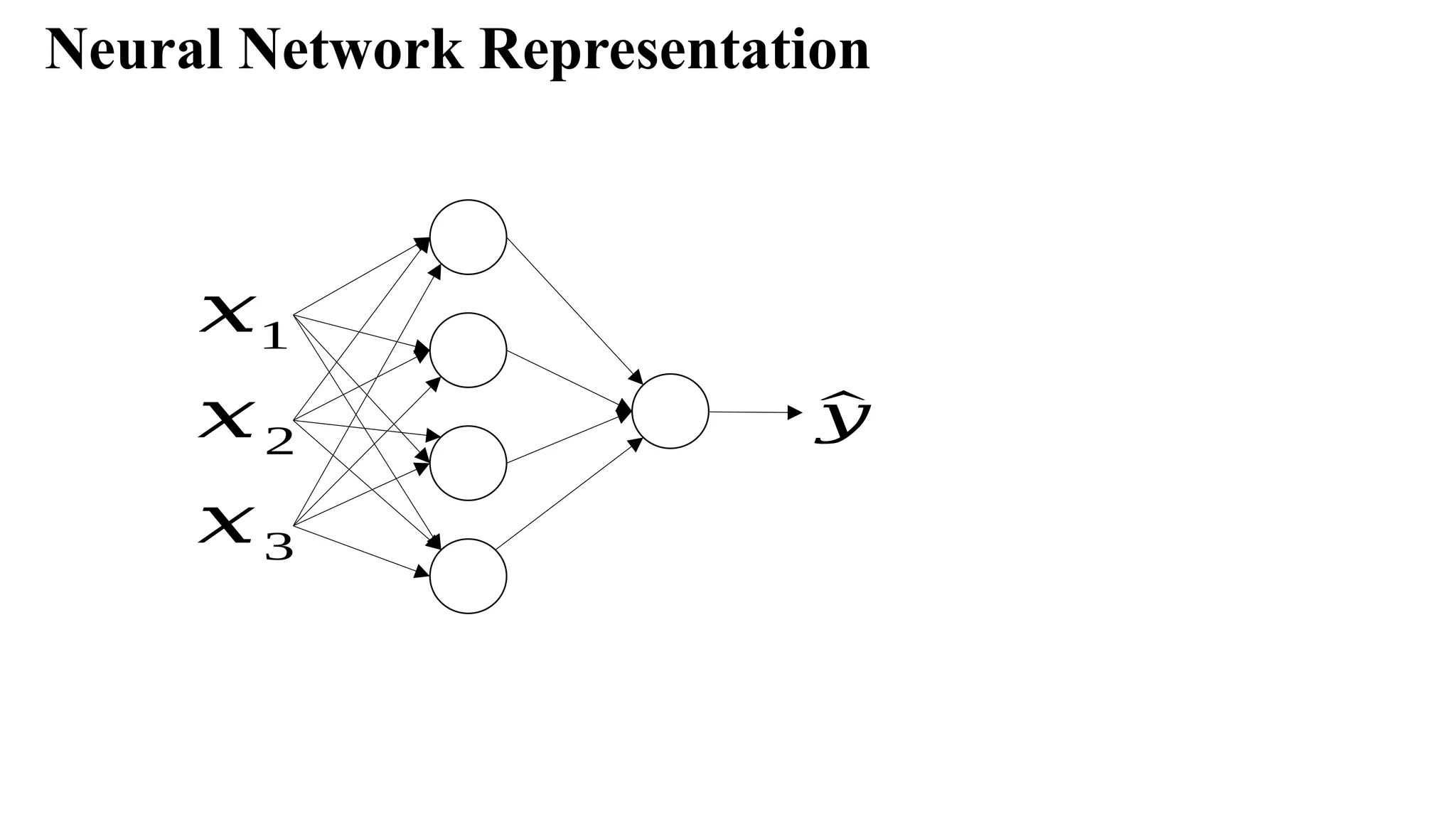
Consider the following representation of Neural Network.
 It has two layers i.e., one hidden layer and one output layer.
 The first layer is referred as a[0]
, second layer as a[1]
, and the final layer as a[2]
. Here ‘a’
stands for activations.
 The corresponding parameters are w[1]
, b[1]
and w[1]
, b[2]

Computing a Neural Network’s Output
𝑥1
𝑥2
𝑥3
^
𝑦
𝑧=𝑤𝑇
𝑥+𝑏
𝑤𝑇
𝑥 +𝑏
𝑎
𝑥1
𝑥2
𝑥3
𝜎 (𝑧) 𝑎= ^
𝑦
𝑧
𝑎=𝜎(𝑧)
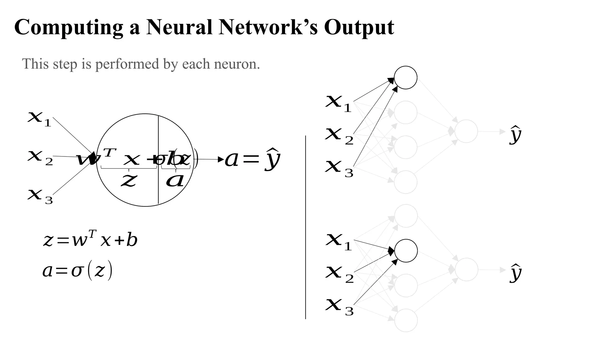
Let’s look in detail at how each neuron of a neural network works. Each neuron takes an input,
performs some operation on them (calculates z = w[T]
+ b), and then applies the activation
function (sigmoid) function:

𝑧=𝑤𝑇
𝑥+𝑏
𝑤𝑇
𝑥 +𝑏
𝑎
𝑥1
𝑥2
𝑥3
𝜎 (𝑧) 𝑎= ^
𝑦
𝑧
𝑎=𝜎(𝑧)
𝑥1
𝑥2
𝑥3
^
𝑦
𝑥1
𝑥2
𝑥3
^
𝑦
This step is performed by each neuron.

𝑥1
𝑥2
𝑥3
^
𝑦
𝑎1
[1 ]
𝑎2
[1 ]
𝑎3
[1 ]
𝑎4
[1 ]
)
)
)
)
This step is performed by each neuron. The equations for the first hidden layer with four
neurons will be:

𝑧[1]
=𝑊[1 ]
𝑥+𝑏[1 ]
𝑎[1 ]
=𝜎 (𝑧[1]
)
𝑧[2 ]
=𝑊[ 2]
𝑎[1]
+𝑏[2 ]
𝑎[2 ]
=𝜎 (𝑧[2 ]
)
𝑥1
𝑥2
𝑥3
^
𝑦
𝑎1
[1 ]
𝑎2
[1 ]
𝑎3
[1 ]
𝑎4
[1 ]
So, for given input X, the outputs for each layer will be:
To compute these outputs, we need to run a for loop which will calculate these values
individually for each neuron. But recall that using a for loop will make the computations very
slow, and hence we should optimize the code to get rid of this for loop and run it faster.

deeplearning.ai
The non-vectorized form of computing the output from a neural network is:
for i=1 to m:
z[1](i) = W[1](i)x + b[1]
a[1](i) = (z[1](i))
𝛔
z[2](i) = W[2](i)x + b[2]
a[2](i) = (z[2](i))
𝛔
Vectorizing across multiple examples
Using this for loop, we are calculating z and a value for each training example separately.
Now we will look at how it can be vectorized. All the training examples will be merged in a
single matrix X:

𝑧
[1] (𝑖)
=𝑊
[1 ]
𝑥
(𝑖)
+𝑏
[1 ]
𝑎
[1 ](𝑖)
=𝜎 (𝑧
[ 1] (𝑖)
)
𝑧
[2 ](𝑖)
=𝑊
[ 2]
𝑎
[ 1](𝑖)
+𝑏
[2]
𝑎
[2 ](𝑖)
=𝜎 (𝑧
[2 ]( 𝑖)
)
Vectorizing across multiple examples
for i = 1 to m:

deeplearning.ai
Activation functions

Activation functions
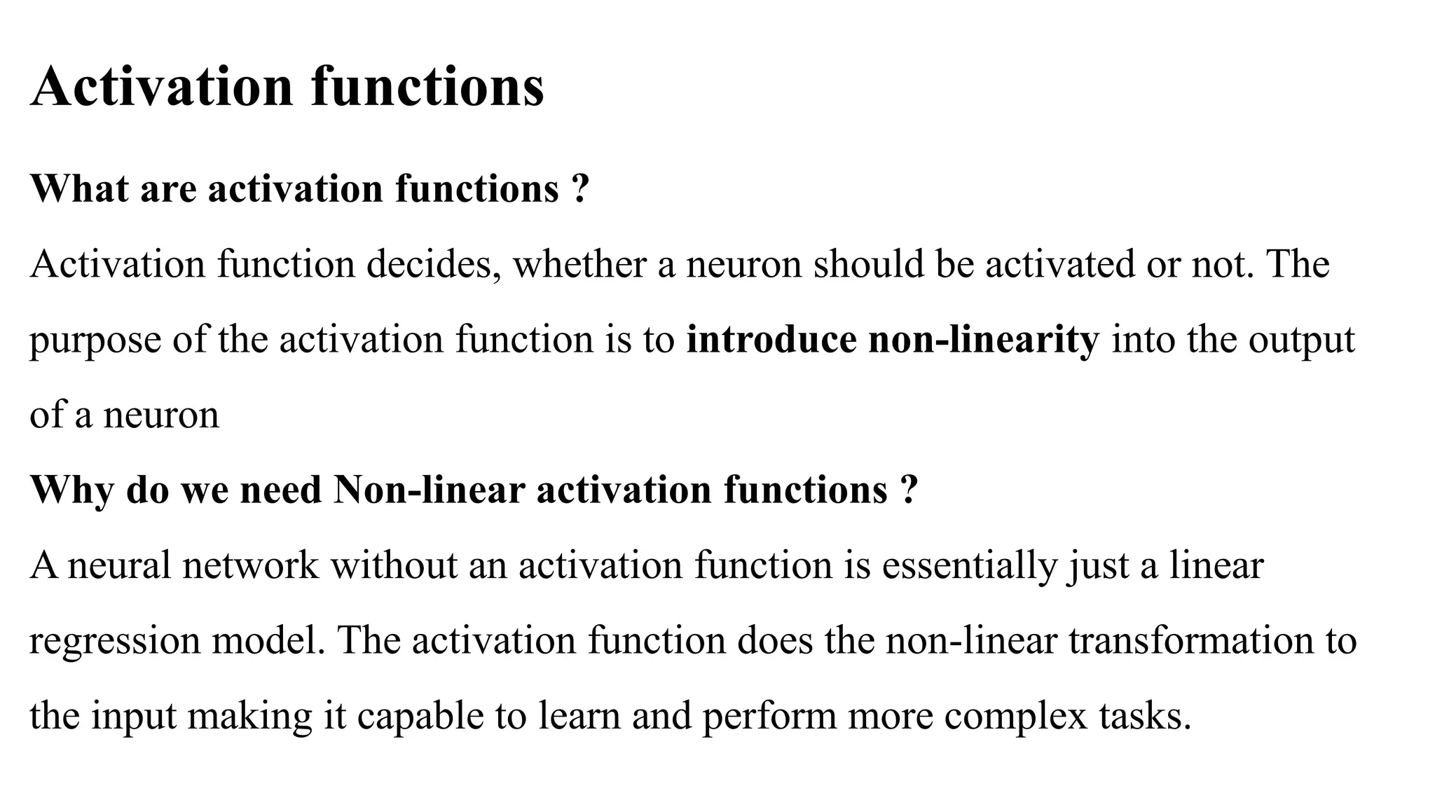
What are activation functions ?
Activation function decides, whether a neuron should be activated or not. The
purpose of the activation function is to introduce non-linearity into the output
of a neuron
Why do we need Non-linear activation functions ?
A neural network without an activation function is essentially just a linear
regression model. The activation function does the non-linear transformation to
the input making it capable to learn and perform more complex tasks.

Sigmoid activation function
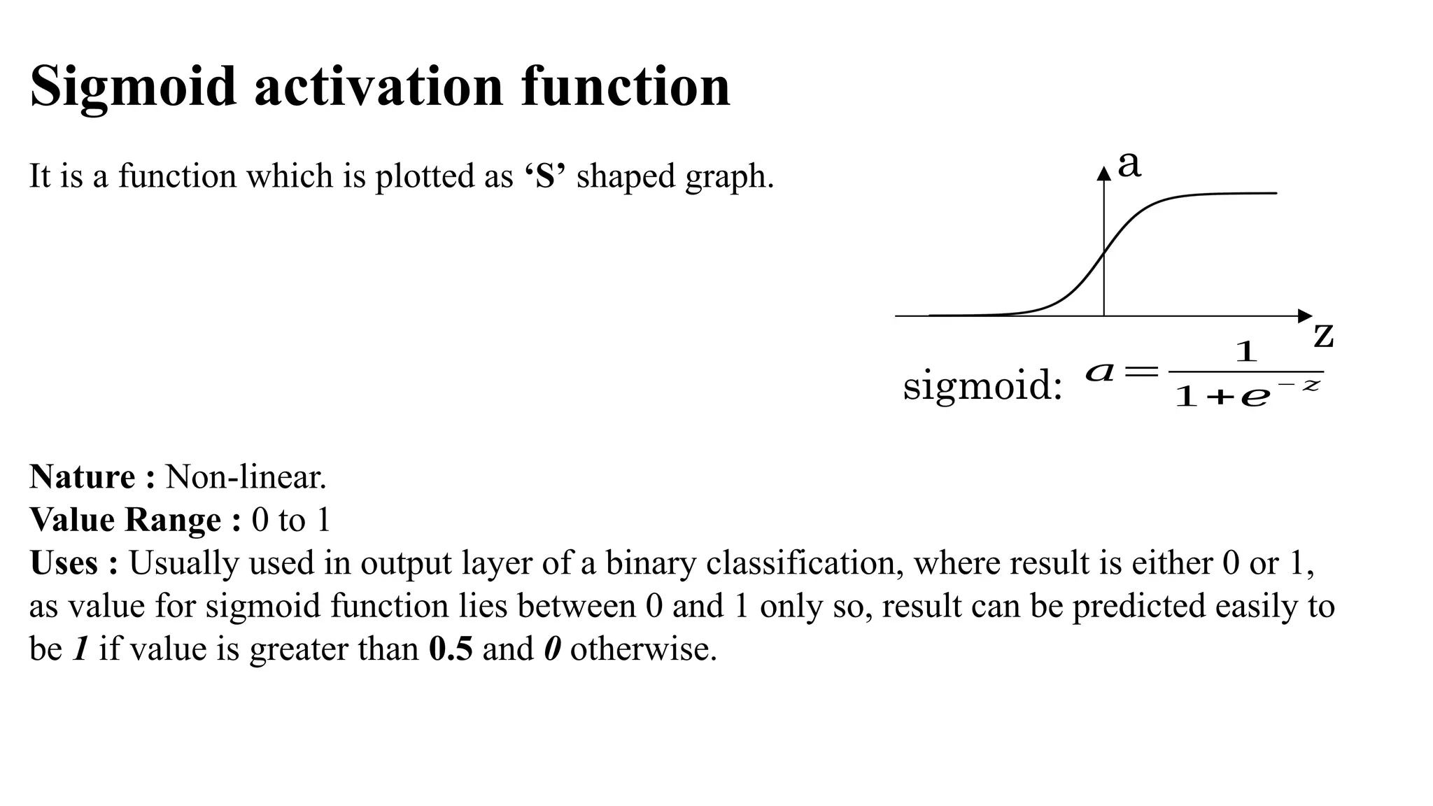
It is a function which is plotted as ‘S’ shaped graph.
Nature : Non-linear.
Value Range : 0 to 1
Uses : Usually used in output layer of a binary classification, where result is either 0 or 1,
as value for sigmoid function lies between 0 and 1 only so, result can be predicted easily to
be 1 if value is greater than 0.5 and 0 otherwise.
a
z
sigmoid: 𝑎=
1
1+𝑒
− 𝑧

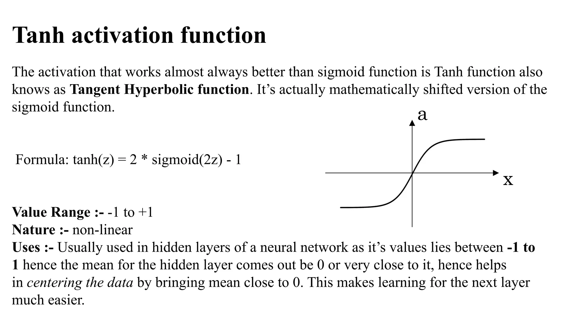
Tanh activation function
The activation that works almost always better than sigmoid function is Tanh function also
knows as Tangent Hyperbolic function. It’s actually mathematically shifted version of the
sigmoid function.
Formula: tanh(z) = 2 * sigmoid(2z) - 1
Value Range :- -1 to +1
Nature :- non-linear
Uses :- Usually used in hidden layers of a neural network as it’s values lies between -1 to
1 hence the mean for the hidden layer comes out be 0 or very close to it, hence helps
in centering the data by bringing mean close to 0. This makes learning for the next layer
much easier.
x
a

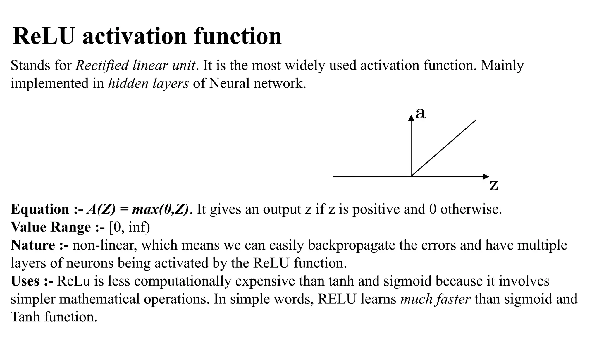
ReLU activation function
Stands for Rectified linear unit. It is the most widely used activation function. Mainly
implemented in hidden layers of Neural network.
Equation :- A(Z) = max(0,Z). It gives an output z if z is positive and 0 otherwise.
Value Range :- [0, inf)
Nature :- non-linear, which means we can easily backpropagate the errors and have multiple
layers of neurons being activated by the ReLU function.
Uses :- ReLu is less computationally expensive than tanh and sigmoid because it involves
simpler mathematical operations. In simple words, RELU learns much faster than sigmoid and
Tanh function.
z
a

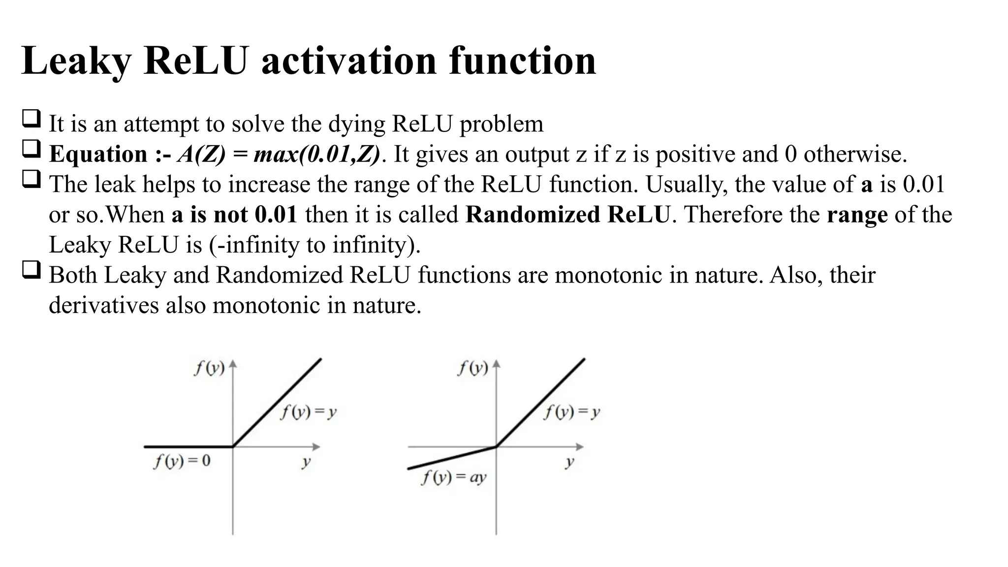
Leaky ReLU activation function
 It is an attempt to solve the dying ReLU problem
 Equation :- A(Z) = max(0.01,Z). It gives an output z if z is positive and 0 otherwise.
 The leak helps to increase the range of the ReLU function. Usually, the value of a is 0.01
or so.When a is not 0.01 then it is called Randomized ReLU. Therefore the range of the
Leaky ReLU is (-infinity to infinity).
 Both Leaky and Randomized ReLU functions are monotonic in nature. Also, their
derivatives also monotonic in nature.

Softmax activation function
 The softmax function is also a type of sigmoid function but is handy when we are trying to
handle classification problems.
 Nature :- non-linear
 Uses :- Usually used when trying to handle multiple classes. The softmax function would
squeeze the outputs for each class between 0 and 1 and would also divide by the sum of the
outputs.
 Output:- The softmax function is ideally used in the output layer of the classifier where we
are actually trying to attain the probabilities to define the class of each input.

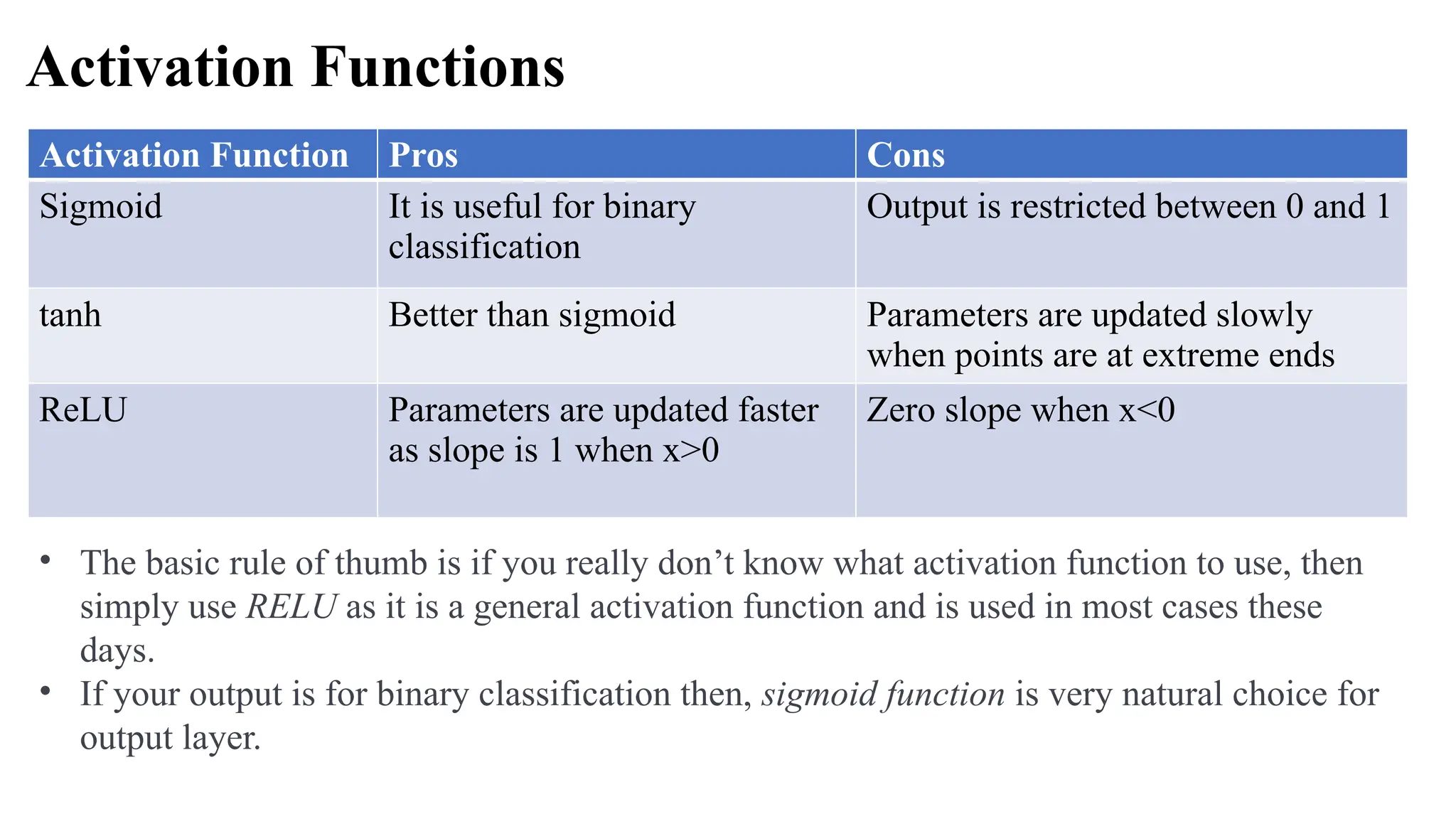
Activation Functions
Activation Function Pros Cons
Sigmoid It is useful for binary
classification
Output is restricted between 0 and 1
tanh Better than sigmoid Parameters are updated slowly
when points are at extreme ends
ReLU Parameters are updated faster
as slope is 1 when x>0
Zero slope when x<0
• The basic rule of thumb is if you really don’t know what activation function to use, then
simply use RELU as it is a general activation function and is used in most cases these
days.
• If your output is for binary classification then, sigmoid function is very natural choice for
output layer.

deeplearning.ai
Gradient descent for neural networks
Backward Pass

deeplearning.ai
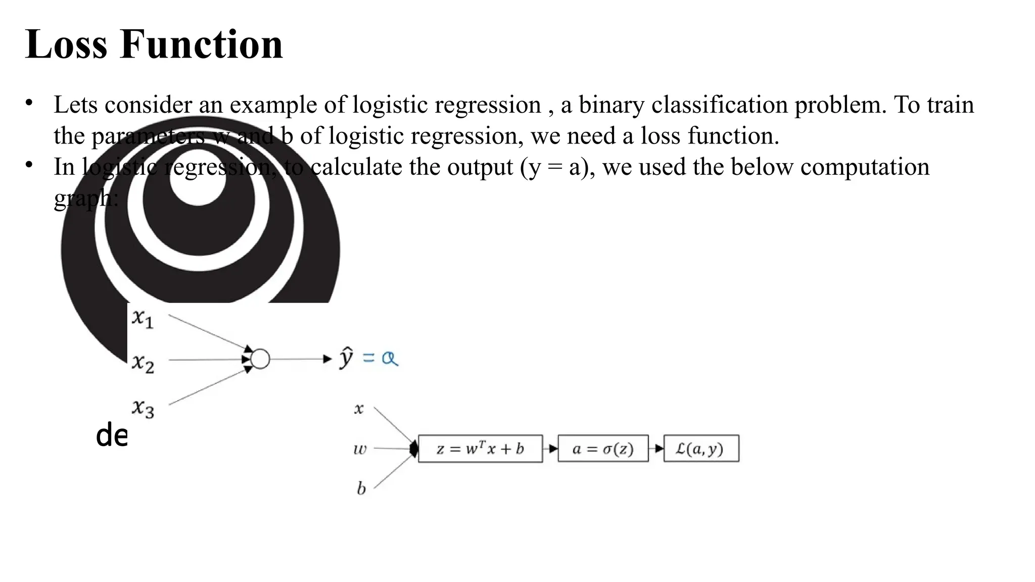
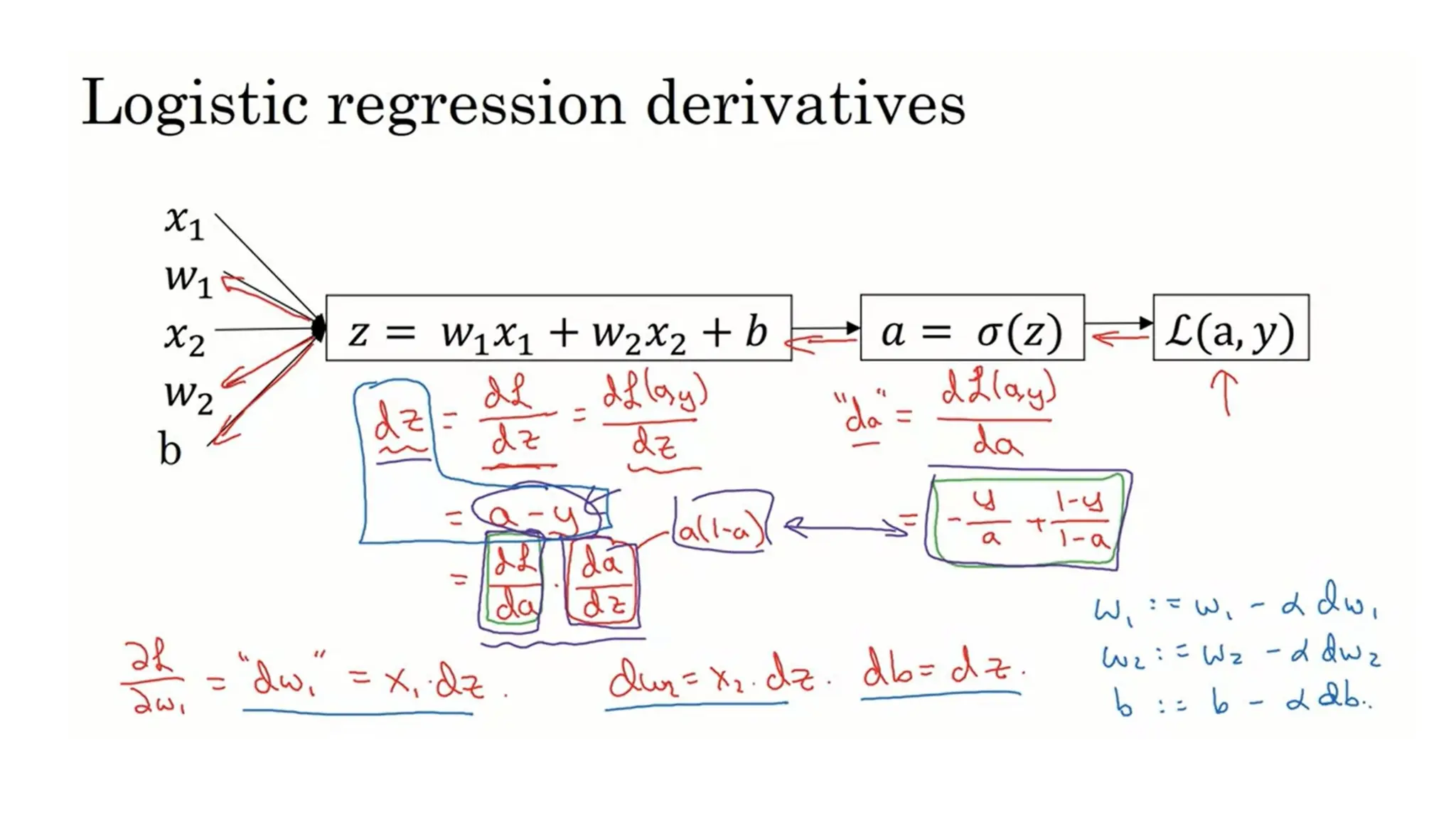
• Lets consider an example of logistic regression , a binary classification problem. To train
the parameters w and b of logistic regression, we need a loss function.
• In logistic regression, to calculate the output (y = a), we used the below computation
graph:
Loss Function

deeplearning.ai
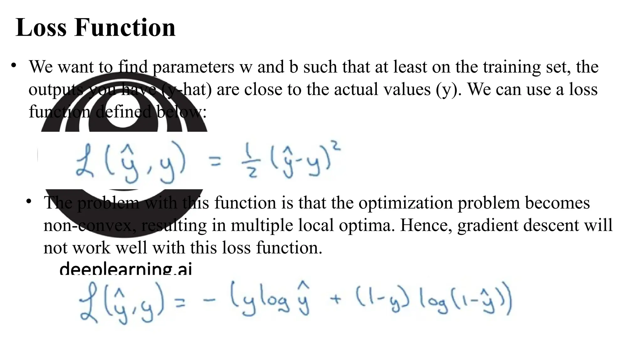
• We want to find parameters w and b such that at least on the training set, the
outputs you have (y-hat) are close to the actual values (y). We can use a loss
function defined below:
Loss Function
• The problem with this function is that the optimization problem becomes
non-convex, resulting in multiple local optima. Hence, gradient descent will
not work well with this loss function.

deeplearning.ai
Cost Function
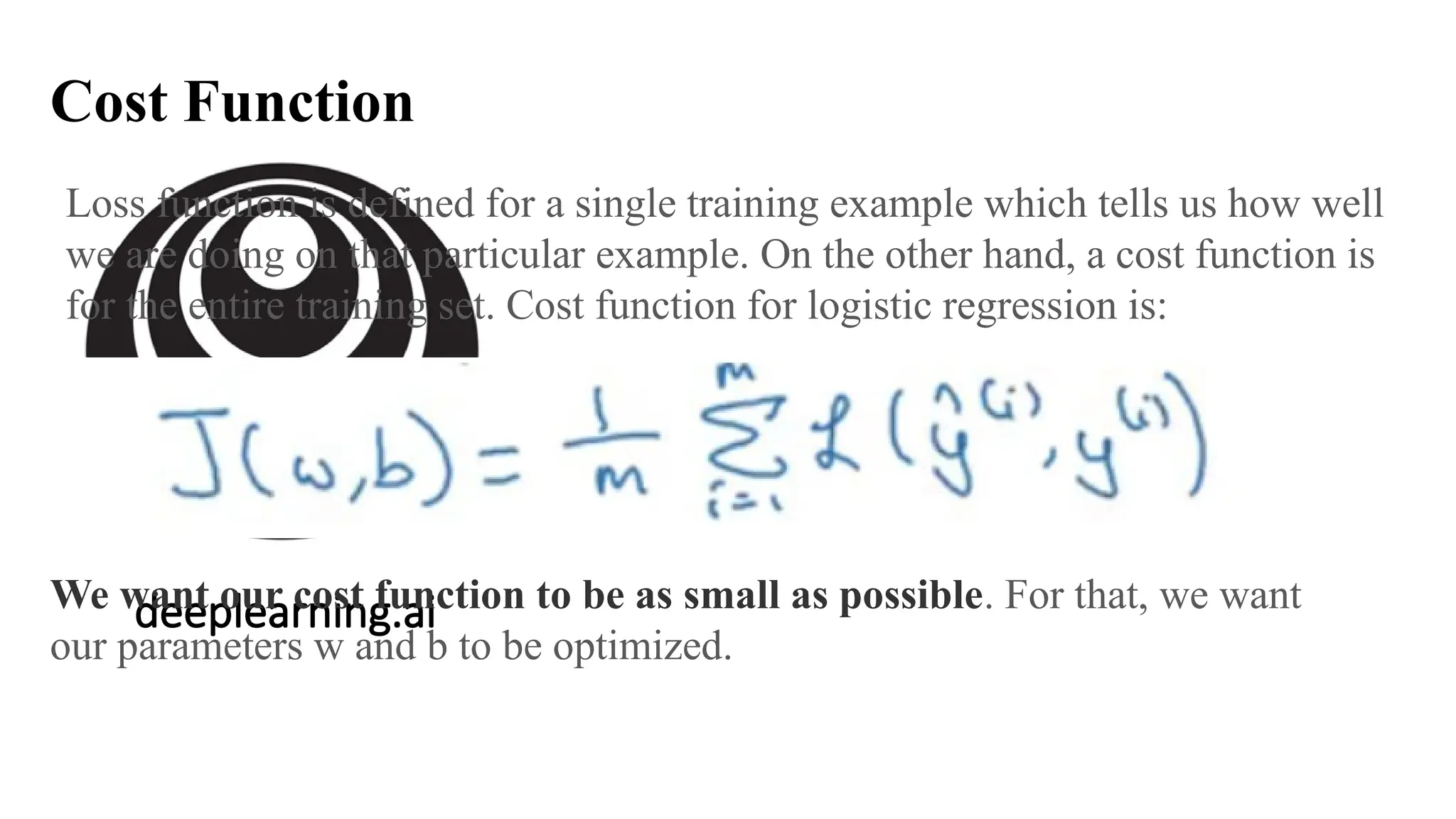
Loss function is defined for a single training example which tells us how well
we are doing on that particular example. On the other hand, a cost function is
for the entire training set. Cost function for logistic regression is:
We want our cost function to be as small as possible. For that, we want
our parameters w and b to be optimized.

deeplearning.ai
Gradient Descent
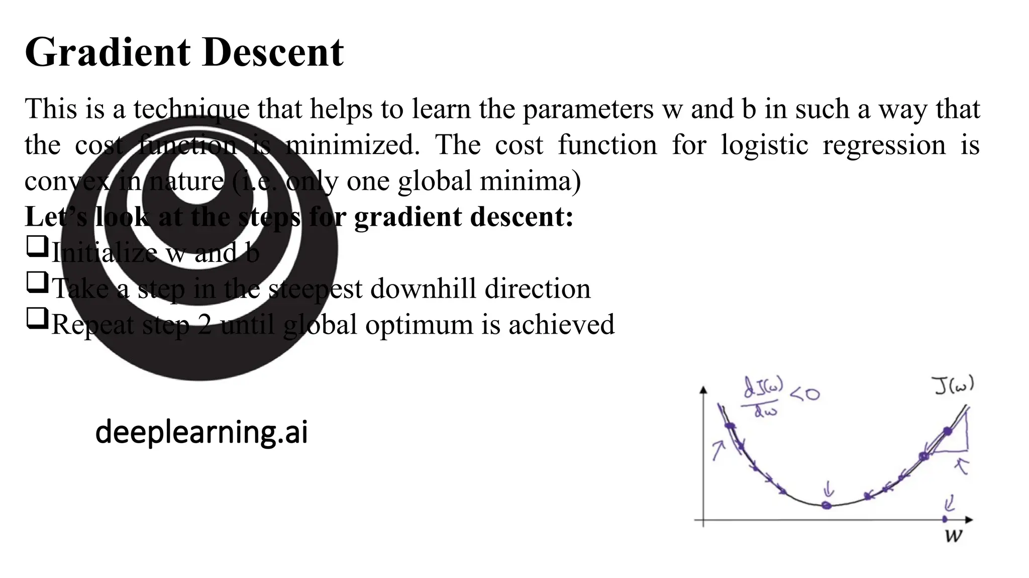
This is a technique that helps to learn the parameters w and b in such a way that
the cost function is minimized. The cost function for logistic regression is
convex in nature (i.e. only one global minima)
Let’s look at the steps for gradient descent:
Initialize w and b
Take a step in the steepest downhill direction
Repeat step 2 until global optimum is achieved

deeplearning.ai
Gradient Descent
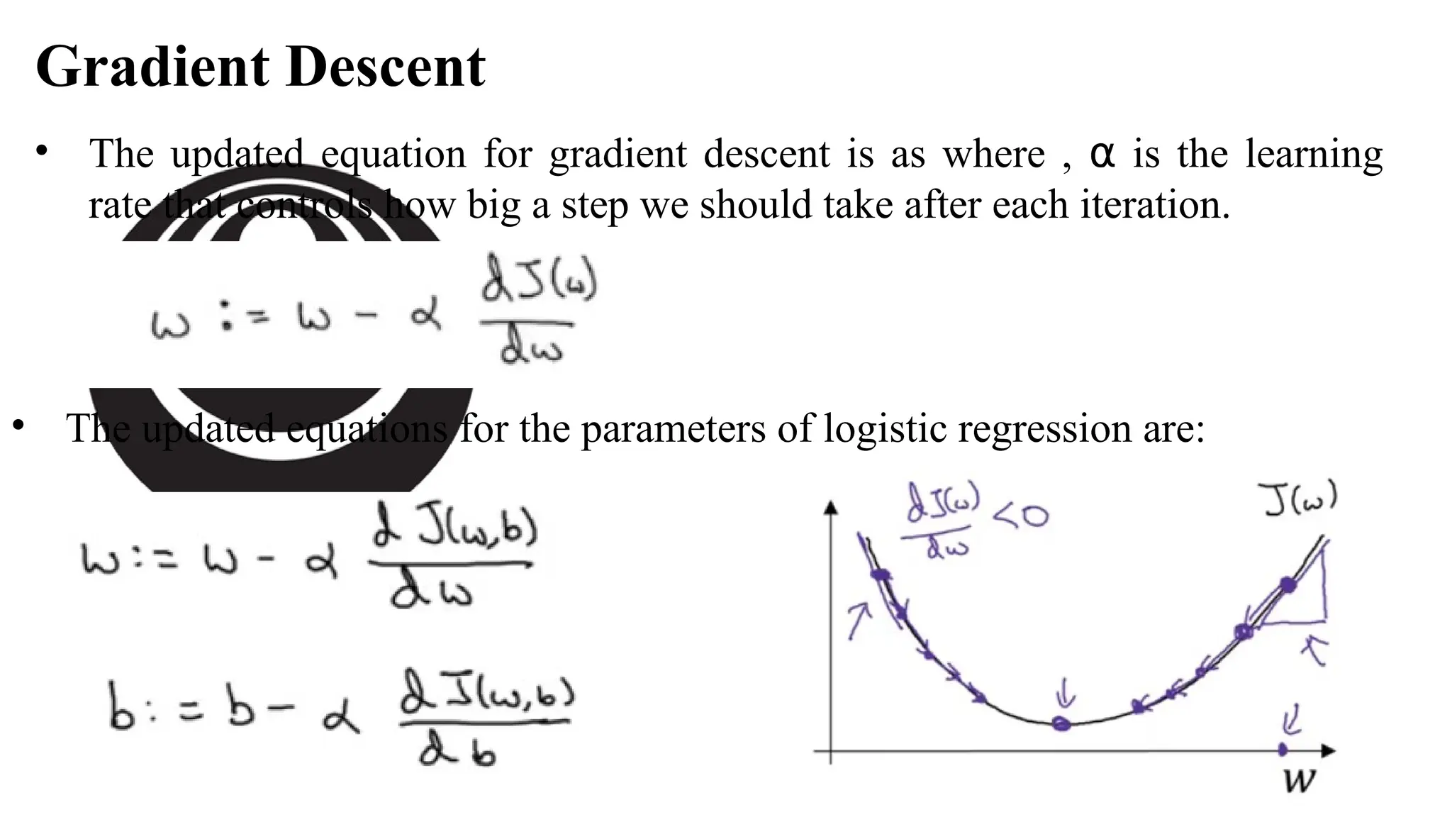
• The updated equation for gradient descent is as where , is the learning
⍺
rate that controls how big a step we should take after each iteration.
• The updated equations for the parameters of logistic regression are:

deeplearning.ai
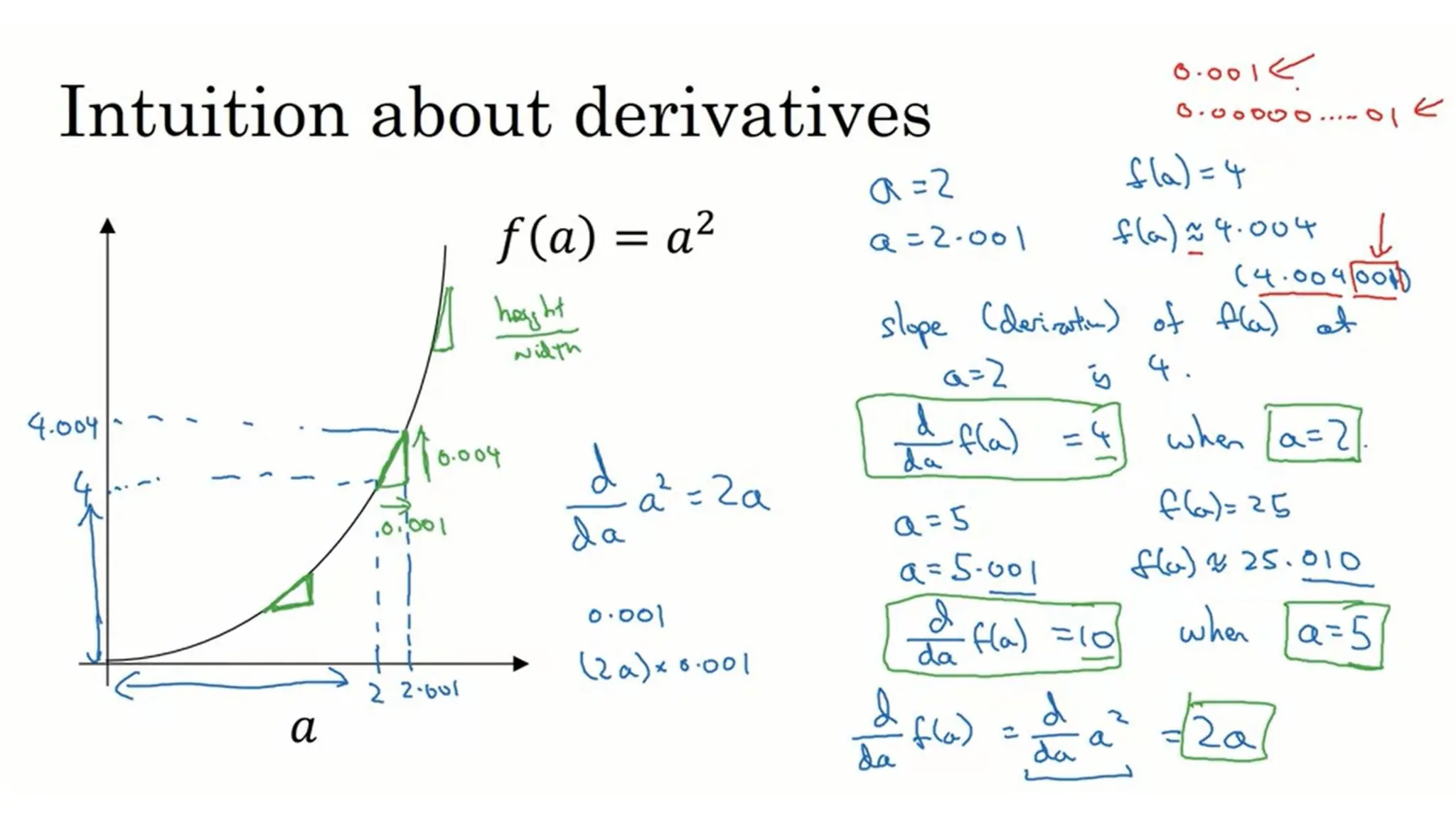
Intuition about derivatives
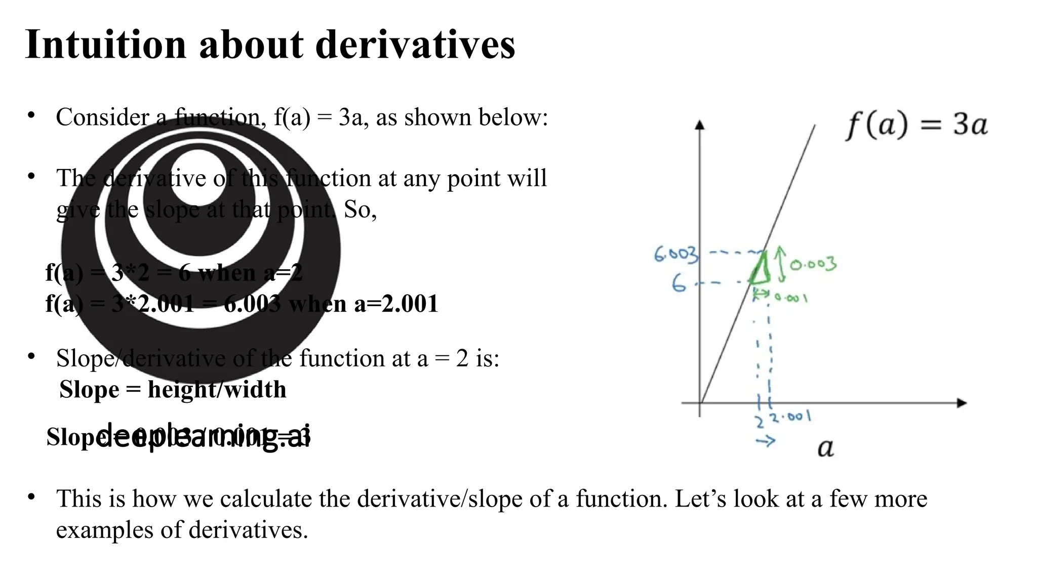
• Consider a function, f(a) = 3a, as shown below:
• The derivative of this function at any point will
give the slope at that point. So,
f(a) = 3*2 = 6 when a=2
f(a) = 3*2.001 = 6.003 when a=2.001
• Slope/derivative of the function at a = 2 is:
Slope = height/width
Slope = 0.003 / 0.001 = 3
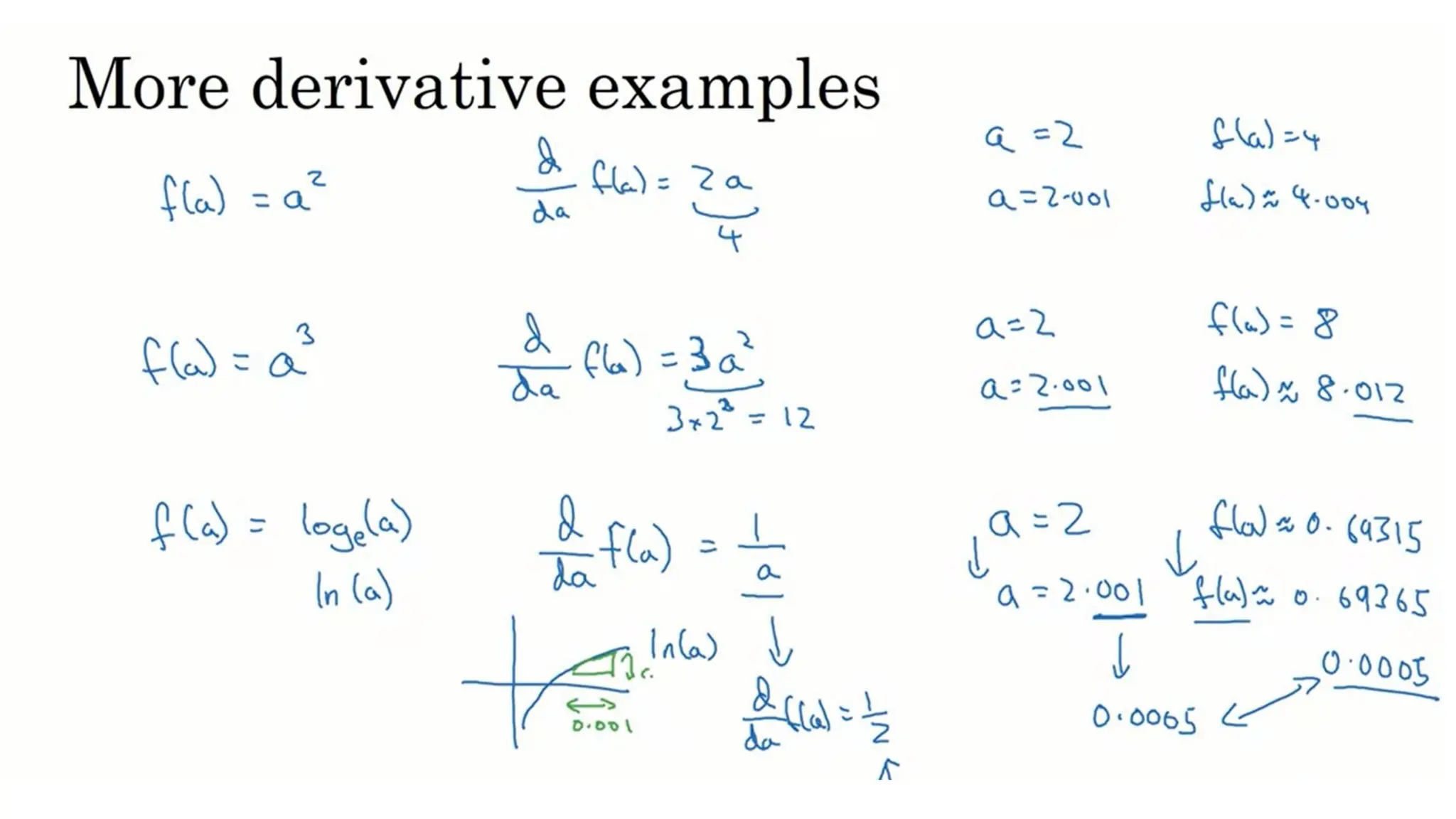
• This is how we calculate the derivative/slope of a function. Let’s look at a few more
examples of derivatives.

deeplearning.ai
f(a) = 3(a+bc)

deeplearning.ai
Vectorization
Vectorization is basically a way of getting rid of for loops in our code. It performs all the
operations together for ‘m’ training examples instead of computing them individually. Let’s
look at non-vectorized and vectorized representation of logistic regression:
Non-vectorized form:
z = 0
for i in range(nx):
z += w[i] * x[i]
z +=b
Now, let’s look at the vectorized form. We can represent the w and x in a vector form:
Now we can calculate Z for all the training examples using:
Z = np.dot(W,X)+b (numpy is imported as np)
The dot function of NumPy library uses vectorization by default. This is how we can vectorize
the multiplications. Let’s now see how we can vectorize an entire logistic regression algorithm.

deeplearning.ai
Broadcasting in Python
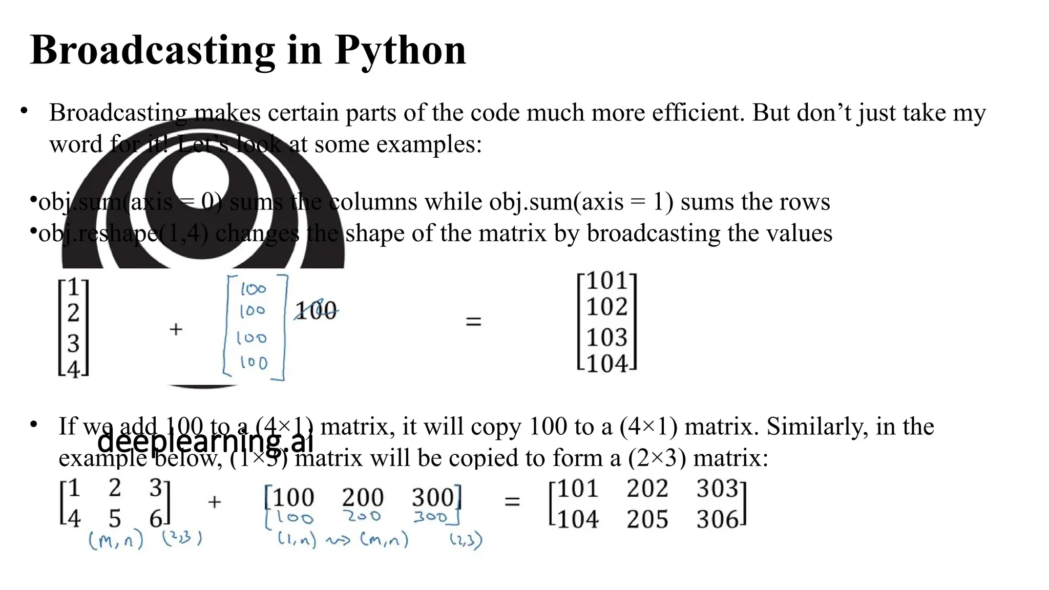
• Broadcasting makes certain parts of the code much more efficient. But don’t just take my
word for it! Let’s look at some examples:
•obj.sum(axis = 0) sums the columns while obj.sum(axis = 1) sums the rows
•obj.reshape(1,4) changes the shape of the matrix by broadcasting the values
• If we add 100 to a (4×1) matrix, it will copy 100 to a (4×1) matrix. Similarly, in the
example below, (1×3) matrix will be copied to form a (2×3) matrix:

deeplearning.ai
Broadcasting in Python
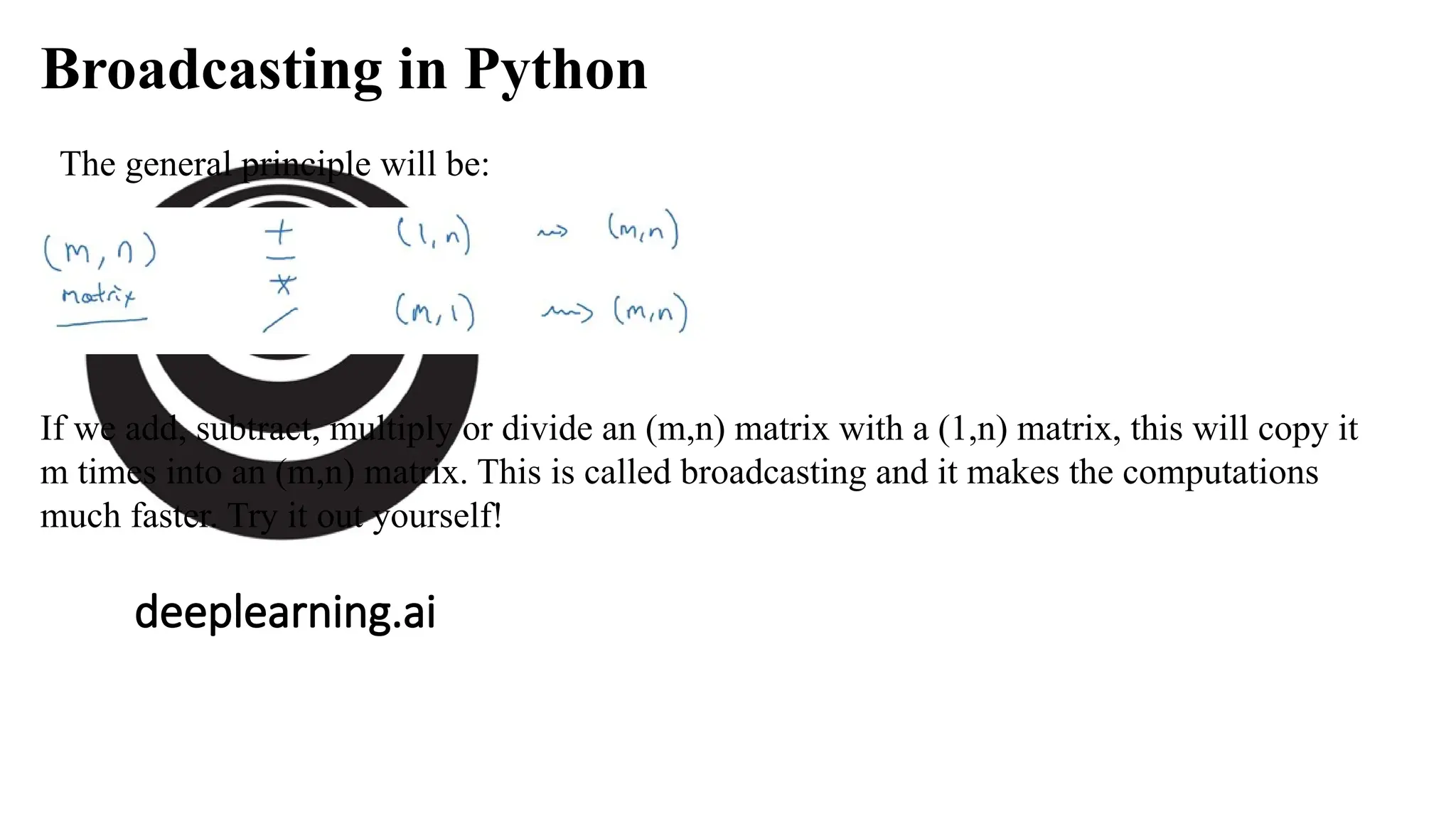
The general principle will be:
If we add, subtract, multiply or divide an (m,n) matrix with a (1,n) matrix, this will copy it
m times into an (m,n) matrix. This is called broadcasting and it makes the computations
much faster. Try it out yourself!

deeplearning.ai
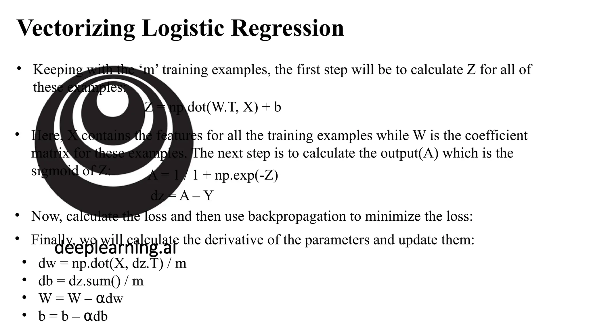
Vectorizing Logistic Regression
• Keeping with the ‘m’ training examples, the first step will be to calculate Z for all of
these examples:
Z = np.dot(W.T, X) + b
• Here, X contains the features for all the training examples while W is the coefficient
matrix for these examples. The next step is to calculate the output(A) which is the
sigmoid of Z: A = 1 / 1 + np.exp(-Z)
• Now, calculate the loss and then use backpropagation to minimize the loss:
dz = A – Y
• Finally, we will calculate the derivative of the parameters and update them:
• dw = np.dot(X, dz.T) / m
• db = dz.sum() / m
• W = W – dw
⍺
• b = b – db
⍺

deeplearning.ai
The parameters which we have to update in a two-layer neural network are: w[1],
b[1], w[2] and b[2], and the cost function we will be minimized. The gradient
descent steps can be summarized as:
Gradient descent

deeplearning.ai
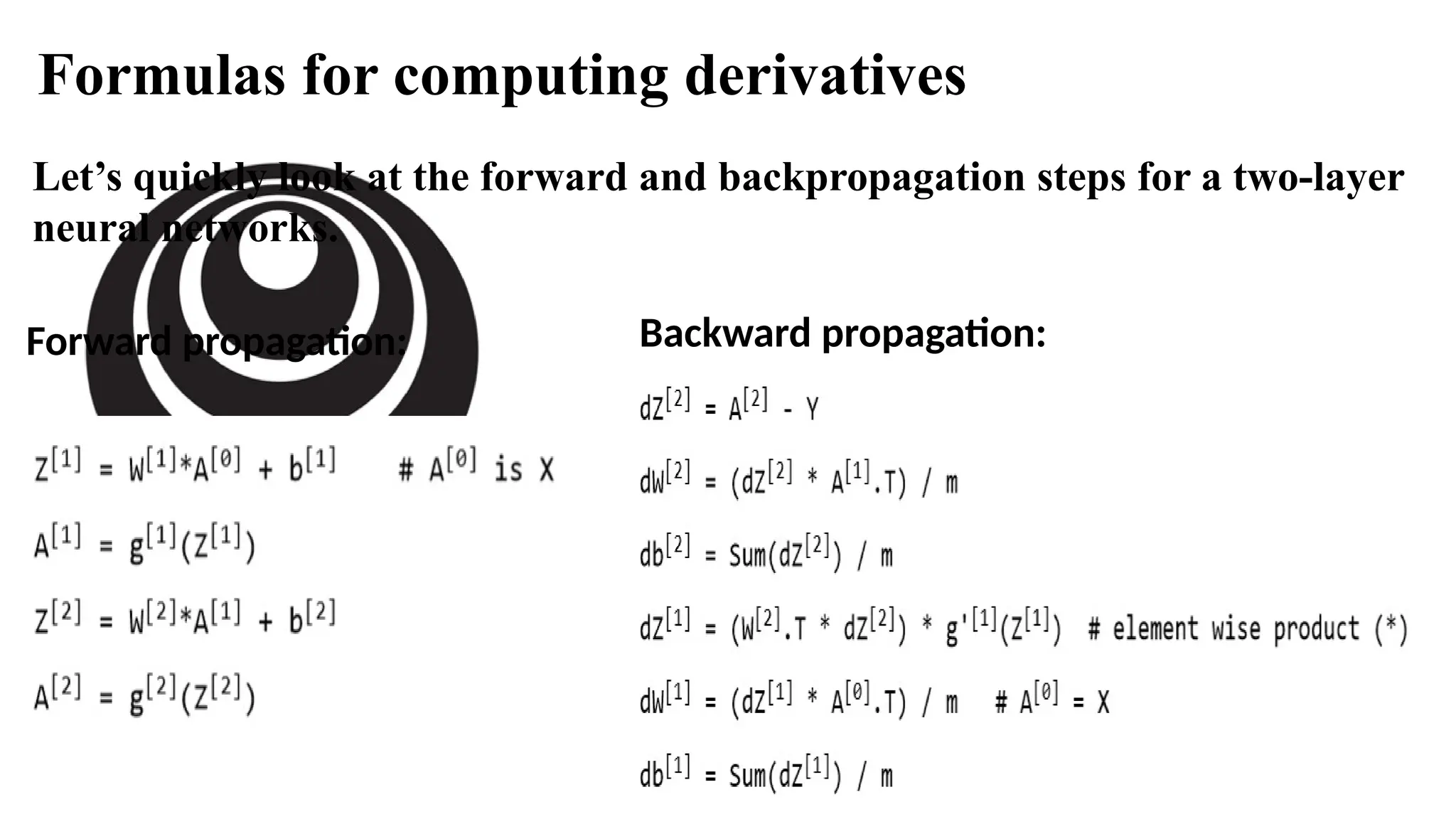
Let’s quickly look at the forward and backpropagation steps for a two-layer
neural networks.
Formulas for computing derivatives
Forward propagation: Backward propagation:

deeplearning.ai
Random Initialization of weights

What happens if you initialize weights to zero?
𝑎1
[1]
𝑥1
𝑎2
[1]
𝑥 2
^
𝑦
𝑎1
[2 ]
 We have previously seen that the weights are initialized to 0 in case of a logistic
regression algorithm. But should we initialize the weights of a neural network to 0? It’s a
pertinent question. Let’s consider the example shown below:
 If the weights are initialized to 0, the W matrix will be:
 Using these weights:
 And finally at the backpropagation step:

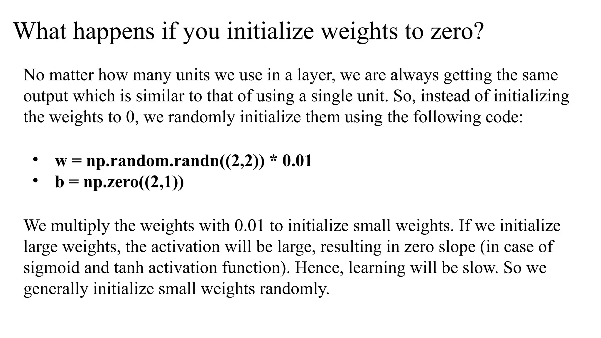
What happens if you initialize weights to zero?
No matter how many units we use in a layer, we are always getting the same
output which is similar to that of using a single unit. So, instead of initializing
the weights to 0, we randomly initialize them using the following code:
• w = np.random.randn((2,2)) * 0.01
• b = np.zero((2,1))
We multiply the weights with 0.01 to initialize small weights. If we initialize
large weights, the activation will be large, resulting in zero slope (in case of
sigmoid and tanh activation function). Hence, learning will be slow. So we
generally initialize small weights randomly.

deeplearning.ai
References
 https://www.coursera.org/specializations/deep-learning
 https://www.geeksforgeeks.org/activation-functions-neural-networks/
 https://www.analyticsvidhya.com/blog/2018/10/introduction-neural-networks-deep-lear
ning
/
 Charu C. Aggarwal, Neural Networks and Deep Learning, A Text Book

Lecture02_Updated_Shallow Neural Networks.pptx

More Related Content

Similar to Lecture02_Updated_Shallow Neural Networks.pptx

Recently uploaded

Lecture02_Updated_Shallow Neural Networks.pptx