1. 8/22/2012
Considerations for determining
Null /Alternative hypothesis
• Error rejecting null hypothesis (when it is
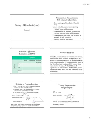
Testing of Hypothesis (cont) true)
is more critical than error in not rejecting
• ‘Default’ is the null hypothesis
Session15
• Hypothesis that is ‘assumed’ to be true till
‘proven’ otherwise is the null hypothesis
• Hypothesis that one would ‘like’ to prove as
wrong is the null hypothesis
2
• Equality should be part of null
Statistical Hypothesis
Practice Problem
Estimation and TOH
Parameter Grant, Inc., a manufacturer of women’s dress blouses,
knows that its brand is carried in 19 percent of the
mean proportion Standard women’s clothing stores east of the Mississippi River.
deviation Grant recently sampled 85 women’s clothing stores on
Single the West Coast and found that 14.12 percent of the
Population
stores carried the brand. At the 0.04 level of
Two
significance, is there evidence that Grant has poorer
distribution on the West Coast than it does east of the
Multiple
Mississippi?
Solution to Practice Problem
• H0 : π = 0.19 and H1: π < 0.19 (π proportion of stores in
Testing for proportion
the west cost which carries the brand) (large sample)
• hypothesis about π; one sample problem; n=85 (large);
one-tailed test; no assumption (use CLT)
• Test statistic isZ = p − 0.19 which is N(0,1) under H0. H0 :π = π 0
.19 × .81
85 p −π0
•Given α=0.04, the C.R. is Z < - 1.75 Test Statistic Z =
•Observed value of the T.S. .1412 − 0.19 = −1.15 > −1.75 π 0 (1 − π 0 )
.19 × .81
85 n
–does not fall in the C.R x which has standard normal distribution
-1.75
•Fail to reject H0 at 4% level of significance and conclude that when H 0 is true
proportion of stores in the west that carry the blouse is NOT
significantly lower than the same in the east.
1

2. 8/22/2012
Two Kinds of Problems in Testing
Power of a test
hypothesis
= Chance of Rejecting H0 when H1 is true
• You are asked to devise a test and give a = Probability[T.S. falls in the critical region|H1]
decision at a given level of significance (or = 1- P(Type II error)
using a p-value approach)
H 0 : µ = µ0 vs H1 : µ < µ0
• The decision rule (when to reject or accept
the null hypothesis) is given and you are
asked to find the prob of Type I/II error or
the power
µ1 µ1 µ0
Power
• Calculation is based on the distribution of TS when H1 is true. Power calculation: Medworld
mu0 100 100
• Make suitable adjustments sigma 3.5 3.5
• Exercise: Do this at least for all one-sample problems n 50 50
• Examples SE 0.495 0.495
– Problem 3: what are the chances of floating the telescopes when the
true SD is 1.9, 1.75, 1.5, 1, … etc alpha 0.05 0.01
– Problem 2: what are the powers of the 4% significance level test if the z-value -1.645 -2.33
actual % of west coast stores carrying the item is 15%, 10%, 5%, etc. cutoff 99.19 98.85
– Problem 1: The mean problem – we can not do it (at this level) only
with pop SD known. Otherwise , would need non-central t distribution. mu1 power power
– Medworld Problem 99.9 0.075 0.017
99.8 0.107 0.027
• Tables have limitation; so we may not get the exact value 99.7 0.149 0.043
always 99.6 0.201 0.064
99.5 0.263 0.094
• Exercise: Case: Breaking the windshield 99.4 0.333 0.133
West Coast: Power function/P(Type II error)
Practice Problem 2: east coast vs west coast pi_1 se_pi1 z-value pi_1 beta
• H0 : π = 0.19 and H1: π < 0.19 0.01 0.010792 9.776227 0.01 0
p − 0.19 0.02 0.015185 6.289477 0.02 1.5927E-10
• Test statistic is Z = which is N(0,1) under H0.
.19 × .81 0.03 0.018503 4.62128 0.03 1.9069E-06
85 0.04 0.021255 3.552454 0.04 0.00019083
•Given α=0.04, the C.R. is Z < - 1.75, or equivalently p < 0.1155 0.05 0.023639 2.771069 0.05 0.00279363
The power of this test (when π =0.10) is 0.06 0.025759 2.154835 0.06 0.01558736
0.07 0.027675 1.644345 0.07 0.05005253
0.08 0.029426 1.206643 0.08 0.11378474
0.09 0.031041 0.821711 0.09 0.20562068
p − 0.1 0.1155 − 0.1
P[ p < 0.1155 | π = 0.1] = P[ < = .47] = 0.6808 0.1 0.03254 0.476544 0.1 0.31684335
.1× .9 .1× .9
0.11 0.033938 0.162255 0.11 0.43555265
85 85
0.12 0.035247 -0.12748 0.12 0.5507216
0.13 0.036477 -0.39733 0.13 0.65443752
0.14 0.037636 -0.6508 0.14 0.74241159
0.15 0.03873 -0.89062 0.15 0.81343272
0.16 0.039764 -1.11894 0.16 0.86841668
2

3. 8/22/2012
West Coast: Power function/P(Type II error)
1.2
Power in Telescope problem
15.4541 0.02 sig0 2 2
1
n 30 30
df 29 29
alpha 0.05 0.01
0.8
chi-sq cut 17.708 14.26
cutoff S 1.5629 1.402
0.6 beta sig1 power power
power
1.9 0.0957 0.022
1.8 0.1741 0.048
0.4
1.7 0.2966 0.099
1.6 0.4644 0.191
0.2
1.5 0.6569 0.34
1.4 0.8305 0.54
1.3 0.9428 0.751
0
0.01 0.02 0.03 0.04 0.05 0.06 0.07 0.08 0.09 0.1 0.11 0.12 0.13 0.14 0.15 0.16 0.17 0.18 0.19 1.2 0.989 0.909
1.1 0.9991 0.982
1.2
Practice Problem:
1
Comparing Friday with Thursday
0.8
On Friday, 11 stocks in a random sample of 40 of the roughly 2500
stocks traded on NYSE advanced. In a sample of 60 stocks taken on
0.6 power: 5% level test
Thursday, 24 advanced. At α=0.10, can you conclude that a smaller
power: 1% level test
Proportion of stocks advanced on Friday than did on Thursday?
0.4
Two sample problems
Comparing proportion/mean/variance of two populations
0.2
Based on independent samples from the two population
0
0.6 0.7 0.8 0.9 1 1.1 1.2 1.3 1.4 1.5 1.6 1.7 1.8 1.9 2
Friday vs. Thursday (modified)
Confidence Intervals for
Q. What is the difference between Friday and Thursday in terms of
π1-π2
the percentage of stocks in NYSE that advance? Give a range which
has 90% chance of containing this difference.
100(1-α)% C.I. for π 1 - π 2 is :
11 24 p1 (1 − p1 ) p (1 − p2 )
pF =
40
= 0.275 pT =
60
= 0.40 Want 90%C.I. of π T − π F p1 − p2 ± Zα × + 2
2 n1 n2
0.4 × 0.6 0.275 × 0.725
(0.40 − 0.275) ± 1.645 × 60
+
40
Valid when the two samples are drawn independently and
two sample sizes n1 and n2 are large
3

4. 8/22/2012
Friday vs. Thursday TOH Testing Hypothesis: Comparison of proportion in two
populations (both sample sizes large)
H 0 : π1 = π 2
Test at α = 0.10, H0 : π T = π F vs H1 : π T > π F
p1 − p2
Test Statistic: p − pF Test Statistic Z =
Z= T C.R. : Z > 1.28 1 1
SE p (1 − p)  + 
ˆ ˆ
Observed value of TS = 0.125/ ? 0.35 × 0.65 0.35 × 0.65
40
+
60
 n1 n2 
= 1.282
which has standard normal distribution
Pooled estimate of % of stocks advanced (assuming it is the same on
a Thursday or a Friday): 11 + 24
= 0.35 when H 0 is true
40 + 60 n1 p1 + n2 p2
Pooled estimate of p =
ˆ
n1 + n2
P-value just marginally less than 0.1. So reject H0 at 10% level of significance
Problem of
Statistical Hypothesis “expensive” wives/ “poor” husbands
Estimation and TOH To celebrate their first anniversary, Randy Nelson decided to
Parameter buy a pair of diamond earrings for his wife Debbie. He was
shown nine pairs with marquise gems weighing approximately
mean proportion Standard 2 carats per pair. Because of differences in colors and qualities
deviation of the stones, the prices varied from set to set. The average
Single price was $2,990, and the standard deviation was $370. He
√ √ √ also looked at six pairs with pear-shaped stones of the sample
Population
2-carat approximate weight. These earrings had an average
Two price of $3,065, and the standard deviation was $805. On the
√ √
basis of this evidence, can Randy conclude (at a significance
level of 0.05) that pear-shaped diamonds cost more, on average,
Multiple
then marquise diamonds?
Modified Problem of
“expensive” wives/ “poor” husbands Two-sample TOH for mean
To celebrate their first anniversary, Randy Nelson decided to when both sample sizes are large
buy a pair of diamond earrings for his wife Debbie. He was
shown 90 pairs with marquise gems weighing approximately
X1 − X 2
2 carats per pair. Because of differences in colors and qualities Test Statistic: Z=
of the stones, the prices varied from set to set. The average S12 S 22
price was $2,990, and the standard deviation was $370. He +
n1 n2
also looked at 60 pairs with pear-shaped stones of the sample
2-carat approximate weight. These earrings had an average
price of $3,165, and the standard deviation was $805. On the
basis of this evidence, can Randy conclude (at a significance
level of 0.05) that pear-shaped diamonds cost more, on average,
then marquise diamonds?
4

5. 8/22/2012
Confidence Intervals for CI for µ1 - µ2
µ1 - µ2 σ1 σ2 unknown , but large samples
100(1-α)% C.I. for µ1 - µ2 is : 100(1-α)% C.I. for µ1 - µ2 is :
σ 2
σ 2
S12 S2
X1 − X 2 ± Zα × 1
+ 2
X1 − X 2 ± Zα × + 2
2 n1 n2 2 n1 n2
Valid when the two samples are drawn independently Valid when the two samples are drawn independently
and σ1 and σ2 are known and σ1 and σ2 are unknown
and and
either (a) two sample sizes n1 and n2 are large Both the sample sizes n1 and n2 are large
or (b) the two population distributions are Normal
Solution to husband-wife problem (original version)
Derivation of Distribution of TS • H0 : µP = µM and H1:µP > µM (µP and µM are average costs of pear-
two sample mean problem •
shaped and marquise diamonds respectively).
hypothesis about means; two sample problem; σ’s unknown
Population SD’s being equal (equal/unequal?) nP=6, nM=9; right-tailed test; assumption: cost of
diamonds (each type) has normal dist. Assume (currently) σ P = σ M
  1 1  X − X 2 − ( µ1 − µ2 ) • Test statistic is X p − XM
X 1 − X 2 ֏ N  µ1 − µ 2 , σ 2 ×  +   ⇒ 1 ֏ N (0,1) T=
ˆ
SE ( X p − X M )
  n1 n2   σ
1 1
+ which has t-distribution with 13 d.f. under H0.
n1 n2
(ni − 1) Si2 (n1 − 1) S12 + (n2 − 1) S 22 •Given α=0.05, the C.R. is T > 1.771
x
֏ χ ni −1 ⇒
2
֏ χ n1 + n2 − 2
2
σ2 σ2 •Observed value of TS 3065 − 2990
= 0.246 < 1.771
X 1 − X 2 − ( µ1 − µ2 ) 5 × 8052 + 8 × 370 2 1 1
⇒ ֏ Tn1 + n2 − 2 ×( + )
(n1 − 1) S12 + (n2 − 1)S 22 1 1 5+8 6 9
+ •does not fall in the C.R
n1 + n2 − 2 n1 n2 •Fail to reject H0 at 5% level of significance and conclude that the pear-shaped
diamonds are not significantly more expensive
Testing for difference of two means Testing for difference of two means
[s.d.’s unknown but equal; [s.d.’s unknown but unequal;
small samples from normal populations] small samples from normal populations]
H 0 : µ1 − µ 2 = d 0
H 0 : µ1 − µ 2 = d 0 X1 − X 2 − d0
Test Statistic T = which has a
X − X 2 − d0 S12 S 2
2
Test Statistic T = 1 which has a +
n1 n2
1 1
Sp + t − distributi on when H 0 is true. The degrees of
n1 n2
freedom is given by
t − distributi on with (n 1 + n 2 − 2) d.f when H 0 is true. S12 2
S2
[ + ]2
S p is a pooled estimate of s.d. from the two groups and n1 n
ν = 2
2
2
( n − 1) S12 + ( n2 − 1) S 2
2
( S )2 × n 1− 1 ( S )2 × n 1− 1
1 2
computed by S = 1 2
p
+
( n1 + n2 − 2) n1 1 n
2 2
5

6. 8/22/2012
Re-do husband/wife problem Paired Comparison of Means between 2
populations
• Samples from the 2 populations are NOT
Since the null hypothesis of equal variance is rejected at 10% level
of significance, we should use the latter method. drawn independently. There is pairing.
The d.f. now turns out to be approximately 9(check!). • Biological/ pharmaceutical tests with
At 5% level of significance, the C.R. is T > 1.833
placebo vs medicine
The observed value of T.S. is
• Is it really 2 sample problem?
X P − X M − d0 3065 − 2990 − 0
= = 0.214
2
S P SM
+
2
8052
+
370 2 • Reduce to 1-sample problem and proceed.
nP nM 6 9
So the conclusion (that the price for pear-shaped diamonds
is not significantly higher on average) stays.
Flow Chart: Two sample TOH of Mean
How can we infer whether σ P = σ M ?
YES YES
Start Independent σ1, σ2
Samples? Known? Z test
Z test
YES NO, NO Use S and S
1 2
Large
paired
YES
F distribution in
sample? n1 n2
Convert to the one-sample Both large? two-sample variance problem
NO problem of mean
T-test NO
T-test
T-test Accept H0
(F-)Test Use S1 and S2
Pooled estimate of σ H0:σ1 = σ2
df = n1+n2-2 Reject H0 df messy
F Distribution How can we infer whether σ P = σ M ?
Sampling Distribution of Ratio of
two sample variances Back to practice Problem 5
2
SP
χa
2
• Test statistic for testing H0 : σ P = σ M is F5,8 = 2
SM
a = Fa ,b
independent
χ b2 The T.S. has a F-distribution (when H0 is true) with d.f.’s
b 5 and 8 respectively. Testing at 10% level of significance, the
C.R. would be F > 3.69 or F < f 5,8,0.95 = 1/ f 8,5,0.05 = 1/4.82
S12 The observed value of T.S. is 805 2
= 4.733 > 3.69
σ 12 370 2
2
has a Fn1 −1,n 2 −1 distribution
S2
So reject the null hypothesis at 10% level of significance
σ2
2
6

7. 8/22/2012
Looking up the F table
C.I. of σ1/ σ2
 SP 2

   1
 1 < σP
2
S2 σ 2 S2 
0.90 = P < 3.69  = P  × M < M < 3.69 × M 
 4.82 S M
2
  4.82 S P σ P
2 2 2
SP 
 σM
2 
 
0 ∝  1
f =? 3.69 S σ S 
= P × M < M < 3.69 × M 
1 1 1  4.82 S P σ P SP 
0.05 = P[ F5,8 < f ] = P[ > ] = P[ F8,5 > ]
F5,8 f f
1 1
So = 4.82 or f =
f 4.82
7