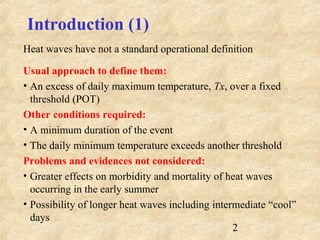
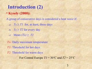
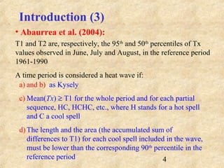
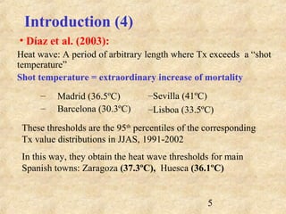
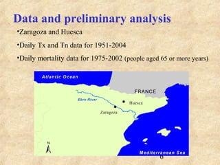
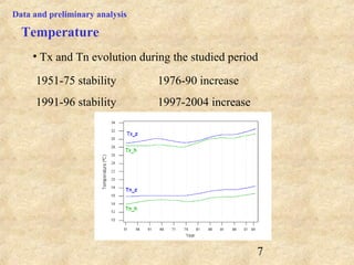
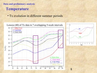
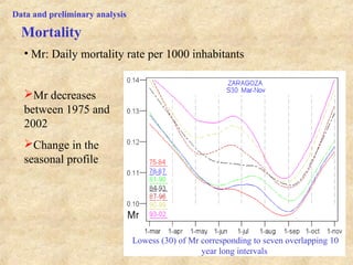
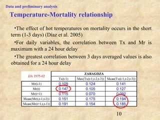
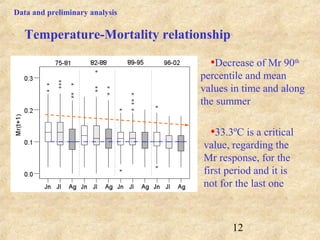
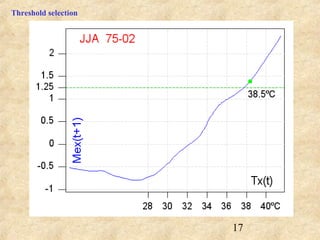
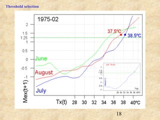
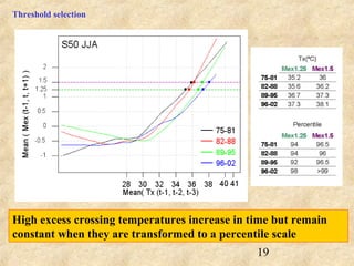
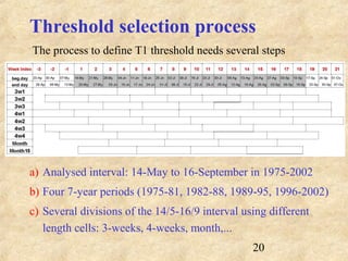
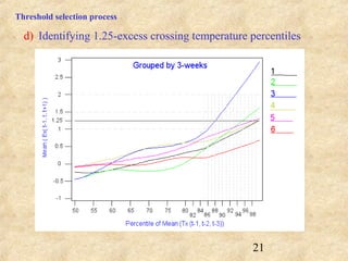
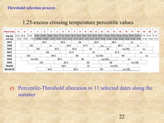
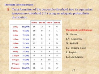
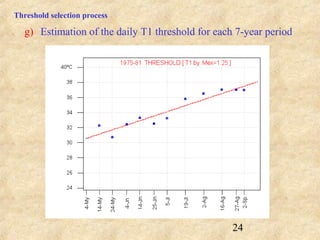
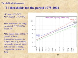
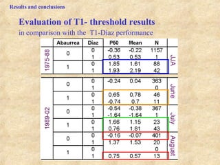
This document discusses definitions of heat waves and methods for determining heat wave thresholds. It analyzes temperature and mortality data from Zaragoza and Huesca, Spain from 1951-2004. A multi-step process is used to define a threshold temperature T1 based on identifying temperature percentiles associated with mortality excesses across time periods. T1 thresholds increase along summer months from 1975-2002 but remain constant when expressed as percentiles. The defined T1 thresholds generally perform better than an alternative definition for identifying periods of elevated mortality risk.

1. 1
9th
International Conference Zaragoza-Pau
on Applied Mathematics and Statistics
On heat wave definition
Abaurrea J., Cebrián A.C., Asín J., Centelles A.
19-21 September 2005

2. 2
Introduction (1)
Heat waves have not a standard operational definition
Usual approach to define them:
• An excess of daily maximum temperature, Tx, over a fixed
threshold (POT)
Other conditions required:
• A minimum duration of the event
• The daily minimum temperature exceeds another threshold
Problems and evidences not considered:
• Greater effects on morbidity and mortality of heat waves
occurring in the early summer
• Possibility of longer heat waves including intermediate “cool”
days

3. 3
• Kysely (2000):
A group of consecutive days is considered a heat wave if:
a) Tx ≥ T1 for, at least, three days
b) Tx ≥ T2 for every day
c) Mean (Tx) ≥ T1
Tx: Daily maximum temperature
T1: Threshold for hot days
T2: Threshold for warm days
For Central Europe T1 = 30ºC and T2 = 25ºC
Introduction (2)

4. 4
a) and b) as Kysely
c) Mean(Tx) ≥ T1 for the whole period and for each partial
sequence, HC, HCHC, etc., where H stands for a hot spell
and C a cool spell
d) The length and the area (the accumulated sum of
differences to T1) for each cool spell included in the wave,
must be lower than the corresponding 90th
percentile in the
reference period
T1 and T2 are, respectively, the 95th
and 50th
percentiles of Tx
values observed in June, July and August, in the reference period
1961-1990
A time period is considered a heat wave if:
Introduction (3)
• Abaurrea et al. (2004):

5. 5
Heat wave: A period of arbitrary length where Tx exceeds a “shot
temperature”
Shot temperature = extraordinary increase of mortality
– Madrid (36.5ºC)
– Barcelona (30.3ºC)
Introduction (4)
• Díaz et al. (2003):
–Sevilla (41ºC)
–Lisboa (33.5ºC)
These thresholds are the 95th
percentiles of the corresponding
Tx value distributions in JJAS, 1991-2002
In this way, they obtain the heat wave thresholds for main
Spanish towns: Zaragoza (37.3ºC), Huesca (36.1ºC)

6. 6
Data and preliminary analysis
•Zaragoza and Huesca
•Daily Tx and Tn data for 1951-2004
•Daily mortality data for 1975-2002 (people aged 65 or more years)

7. 7
Temperature
• Tx and Tn evolution during the studied period
1951-75 stability 1976-90 increase
1991-96 stability 1997-2004 increase
Data and preliminary analysis

8. 8
• Tx evolution in different summer periods
Temperature
Data and preliminary analysis
Lowess (40) of Tx data in 7 overlapping 5-week intervals

9. 9
Lowess (30) of Mr corresponding to seven overlapping 10
year long intervals
Mr decreases
between 1975 and
2002
Change in the
seasonal profile
Mortality
Data and preliminary analysis
• Mr: Daily mortality rate per 1000 inhabitants

10. 10
•The effect of hot temperatures on mortality occurs in the short
term (1-3 days) (Díaz et al. 2005)
•For daily variables, the correlation between Tx and Mr is
maximum with a 24 hour delay
•The greatest correlation between 3 days averaged values is also
obtained for a 24 hour delay
Temperature-Mortality relationship
Data and preliminary analysis

11. 11
Data and preliminary analysis
The impact on Mr of a fixed high temperature
changes in time and along the summer
To show this property we select a temperature value,
33.3ºC, the 90th
percentile of daily Tx values in June, 1975-
81
•1975-02 is divided into four 7-year periods and we
consider observations from June, July and August
Temperature-Mortality relationship

12. 12
Data and preliminary analysis
•Decrease of Mr 90th
percentile and mean
values in time and along
the summer
•33.3ºC is a critical
value, regarding the
Mr response, for the
first period and it is
not for the last one
Temperature-Mortality relationship

13. 13
Data and preliminary analysis
•Decrease of Mr 90th
percentile and mean
values in time and along
the summer
•33.3ºC is a critical
value, regarding the
Mr response, for the
first period and it is
not for the last one
Temperature-Mortality relationship

14. 14
Mortality Excess
We define the mortality excess, Mex(t), in day t as the
difference between the number of deaths, Mf(t), and its
expected value, Me(t)
Mex (t) = Mf(t) –Me(t)
The expected mortality is obtained by fitting a regression
model including:
a) Time terms until the second order (long term evolution)
b) Harmonic terms until the fourth order (seasonality)
c) Dummy variables for indicating the periods 75-86, 87-96
and 97-02, in order to fit different seasonal patterns

15. 15
Expected and observed mortality lowess
Mortality Excesss

16. 16
•We try to identify the ‘shot temperature’ for each 7-year
period and summer interval, looking for the change point in
the lowess smoother of Mex vs. Tx
PROBLEMS
Smoothed curves are frequently erratic because of small
sample sizes
A proper shot temperature doesn’t appear in many
graphs
Threshold selection

17. 17
Threshold selection

18. 18
Threshold selection

19. 19
High excess crossing temperatures increase in time but remain
constant when they are transformed to a percentile scale
Threshold selection

20. 20
Threshold selection process
The process to define T1 threshold needs several steps
a) Analysed interval: 14-May to 16-September in 1975-2002
b) Four 7-year periods (1975-81, 1982-88, 1989-95, 1996-2002)
c) Several divisions of the 14/5-16/9 interval using different
length cells: 3-weeks, 4-weeks, month,...

21. 21
d) Identifying 1.25-excess crossing temperature percentiles
Threshold selection process

22. 22
Threshold selection process
e) Percentile-Threshold allocation to 11 selected dates along the
summer
1.25-excess crossing temperature percentile values

23. 23
f) Transformation of the percentile-threshold into its equivalent
temperature-threshold (T1) using an adequate probabilistic
distribution
Threshold selection process
Probabilistic distributions:
N: Normal
LN: Lognormal
W: Weibull
EV: Extreme Value
L: Logistic
LL: Log-Logistic

24. 24
g) Estimation of the daily T1 threshold for each 7-year period
Threshold selection process

25. 25
•4th
June: 32.3-34ºC
•27th
August: 37-39.8ºC
•The increase of T1 along
the period 1975-2002 is
about 2ºC
•The bigger slope of the 3rd
period is due to
temperature warming in
August and July, whereas
the smaller slope of the 4th
period is due to strong
temperature increase in
June
Threshold selection process
T1 thresholds for the period 1975-2002

26. 26
in comparison with the T1-Díaz performance
Results and conclusions
Evaluation of T1- threshold results

27. 27
References
Abaurrea, J., et al. (2004). Modelling hot extreme temperature events using a
non homogeneous Poisson model. 6th World Congress of Bernoulli Society for
Mathematical Statistics and Probability, Barcelona.
Díaz, J., et al. (2002). Effects of extremely hot days on people older than 65
years in Seville (Spain) from 1986 to 1997. Int. J. Biometeorology, 46, 145-
149.
Díaz, J., Linares, C., García-Herrera, R. (2005). Impacto de las temperaturas
extremas en la salud pública. Futuras actuaciones. Rev. Esp. Salud Pública, 79,
145-157.
Kysely, J. (2002). Temporal fluctuations in heat waves at Prague, the Czech
republic, from 1901-97 and their relationship to atmospheric circulation. Int. J.
Climatol., 22, 33-50.
Robinson, P. J. (2001). On the definition of a heat wave. J. of Applied
Meteorology, 40, 762-75.