This document summarizes a study that measures the cost efficiency of 202 municipalities in the Czech Republic from 2003-2008. It applies both non-parametric and parametric methods to measure efficiency and explain determinants. The key findings are that population size, education levels, capital expenditures, subsidies and revenues influence inefficiency, while more political competition and voter involvement increase efficiency. When analyzing an earlier period (1994-1996), political variables influenced inefficiency differently. Small municipalities improved efficiency more over time than large municipalities.

1. Local Government Efficiency: Evidence from the Czech
Municipalities∗
ˇt
Lenka Sˇastn´†
a Martin Gregor‡
December 15, 2010
Abstract
We measure cost efficiency of 202 Czech municipalities of extended scope in period
2003–2008. The study is the first application of overall efficiency measurement of the
local governments in the new EU member states, and the second in post-communist coun-
tries. We measure government efficiency through established quantitative and qualitative
indicators of the provision of education, cultural facilities, infrastructure and other local
services. First, we employ non-parametric approach of the data envelopment analysis and
adjust the efficiency scores by bootstrapping. Second, we employ the stochastic frontier
analysis and control for effects of various demographic, economic, and political variables.
We compare scores under our preferred specification, i.e. pseudo-translog time-variant
stochastic-frontier analysis with determinants, with alternative scores. The determinants
that robustly increase inefficiency are population size, distance to the regional center, share
of university-educated citizens, capital expenditures, subsidies per capita, and the share
of self-generated revenues. Concerning political variables, increase in party concentration
and the voters’ involvement increases efficiency, and local council with a lower share of
left-wing representatives also tend to be more efficient. We interpret determinants both
as indicators of slack, non-discretionary inputs, and unobservable outputs. The analysis
is conducted also for the period 1994–1996, where political variables appear to influence
inefficiency in a structurally different way. From comparison of the two periods, we obtain
that small municipalities improve efficiency significantly more that large municipalities.
JEL Classification: D24, H72
Keywords: Public spending efficiency, Data Envelopment Analysis, Stochastic Frontier
Analysis, local governments
∗
This research was supported by a grant from the CERGE-EI Foundation under a program of the Global
Development Network. All opinions expressed are those of the authors and have not been endorsed by CERGE-
EI or the GDN. The article benefited from useful comments by Tom Coup´, Libor Duˇek, Randall Filer, Ira
e s
Gang, and Jacek Mercik. We also thank Adam Ander and Nail Hassairi for research assistance.
†
Corresponding author. Ph.D. candidate. Institute of Economic Studies, Faculty of Social Sciences, Charles
University, Opletalova 26, Prague, CZ-110 00; E-mail: stastna@fsv.cuni.cz.
‡
Institute of Economic Studies, Faculty of Social Sciences, Charles University, Opletalova 26, Prague, CZ-
110 00; E-mail: gregor@fsv.cuni.cz.
1

2. 1 Introduction
Efficiency of local public spending is a topic of recent interest in public and urban economics.
For practitioners, robust efficiency measures serve as performance benchmarks that help to
discipline and improve local public management; for academic economists, the production
function approach embedded in the efficiency measures allows to measure and explain the
government’s bias to the production of publicly irrelevant outputs, and separate between
competing explanations why the local governments increase public spending.
In the last two decades, measuring efficiency in local governments became widespread
particularly within individual European countries. Recent evidence is available from Belgium
(Vanden Eeckaut et al. 1993; De Borger, Kerstens 1996; De Borger et al. 1994; for Flanders,
see Geys and Moesen 2009a, 2009b), Finland (Loikkanen, Susiluoto 2005), Germany (Geys et
al. 2010; Kalb 2010), Italy (Boetti et al. 2010), Norway (Borge et al. 2008), Portugal (Afonso,
Fernandes 2006, 2008), and Spain (Arcelus et al. 2007, Balaguer-Coll et al. 2007; Gimenez,
Prior 2007). Out of Europe, recent studies cover, inter alia, the large U.S. cities (Grossman
et al. 1999; Moore et al. 2005), Canadian municipalities (Pollanen 2005) as well as Australian
municipalities (Worthington, Dollery 2002).
There are three reasons to measure efficiency of local governments rather than central
governments: (i) Unlike cross-country comparisons of public sector efficiency, single-country
studies feature relatively consistent statistics and suffer less from unobserved heterogeneity,
hence more likely comply with the restrictive assumption of a homogenous production func-
tion. (ii) Municipalities implement many “state-delegated” powers assigned by the central
government, where the only room for manoeuvre is on the cost side. (iii) At the local level,
policies are more means-focused than ends-focused also because of the absence of many instru-
ments that address the main socio-economic (distributive) conflicts, such as income taxation,
and therefore are more related to the provision of (local) public goods.
We empirically asses cost efficiency of 202 municipalities of extended scope in the Czech
Republic over the period 2003–2008. This period features institutional and territorial stability,
unlike the reform years 2000–2002. By measuring efficiency comprehensively instead by sector-
specific scores, we avoid an issue of fungibility of spending and misclassification into spending
categories that is quite frequent at the local level. To our knowledge, our study is a first
comprehensive local government efficiency exercise in the new EU members states, and the
second in the post-communist region (cf. Hauner 2008). The analysis of determinants allows
us to assess whether patterns of efficiency in municipalities of a post-communist country differ
from those in the culturally and institutionally not so distant Western European countries
(e.g., Belgium, Finland, or Germany); it also permits to briefly observe the evolution in
performance and efficiency from 1990s to 2000s.
We apply both parametric and non-parametric efficiency measurement methods, and also
explain why the most refined parametric method (stochastic frontier analysis with a time-
variant Pseudo-Translog specification and determinants) is, at least in our setting, preferred
to the best non-parametric method (data envelopment analysis with variable returns to scale
and bias corrected by bootstrapping). We end up with efficiency scores and compare with
alternative methodologies. For each individual municipality, our procedure allows to iso-
2

3. late away separately (i) the effect of including determinants and (ii) the effect of assuming
stochastic parametric versus deterministic non-parametric methodology, which is crucial for
the interpretation of individual scores and benchmarking.
This analysis of the slack is conditional on the proper definition of the relevant set of
outputs; we focus on basic services and maintenance of infrastructure, including also selected
quality indicators. As is typical in the literature, the efficiency scores thus have to be inter-
preted as the provision of observable core services. In the parametric approach, we employ
and control for effects of various demographic, economic, and political variables. Important
ones are population size, distance to the regional center, education, fiscal capacity, and lo-
cal political competition. We interpret determinants both as effects upon the slack and the
presence of non-discretionary inputs and unobservable outputs.
With a preferred method, we replicate the analysis also for the period 1994–1996, with a
few changes. The effect of determinants is quite similar, with exception of political variables
that appear to influence inefficiency in a structurally different way. From comparison of the
two periods, we also obtain that small municipalities improve efficiency significantly more that
large municipalities. As a result, initially low differences between efficiency scores, especially
between medium-size and large municipalities, have magnified over time.
The paper proceeds as follows. Section 2 briefly outlines the methodology on estimation
of efficiency scores, and Section 3 presents the dataset. Section 4 gives the non-parametric
results with year-specific scores and their averages. The key Section 5 delivers the parametric
results for panel data with determinants, evaluates the role of determinants, and compares
the available methods. Section 6 analyzes efficiency in 1990s. Section 7 concludes.
2 Methodology
Although discretion exists in many variables in the researcher’s menu of choices, a key decision
in an efficiency estimation is always whether cost efficiency of decision-making units will be
measured in the class of non-parametric or parametric methods. A non-parametric approach
generates the best practice frontier by tightly enveloping the data, where this envelopment is
achieved by solving a sequence of linear programs. The main advantage of the non-parametric
approach is the absence of the apriori specification of the functional form of the frontier. Two
main techniques stand out within the non-parametric approach, Data Envelopment Analysis
(DEA) and Free Disposal Hull Analysis (FDH). DEA, initiated by Farrel (1957) and made
widespread by Charnes et al. (1978), assumes that the production frontier is convex, while
FDH, suggested by Deprins et al. (1984), drops the convexity assumption. These methods
are fully deterministic, and the entire deviation from the frontier is interpreted as inefficiency.
The parametric approaches establish the best practice frontier on the basis of a specific
functional form applied in an econometric estimation. Moreover, the deviations from the best
practice frontier derived from parametric methods can be interpreted in two different ways.
While deterministic approaches interpret the whole deviation from the best practice frontier
as inefficiency (corrected OLS method), stochastic frontier models proposed by Aigner et al.
(1977) and Meeusen and van den Brock (1977) decompose the deviation from the frontier
3

4. into an inefficiency part and a stochastic term. In addition, environmental variables can be
easily treated with a stochastic frontier, whereas two-stage DEA models (e.g., OLS and Tobit
censored regression) ignore serial correlation of efficiency scores(Simar, Wilson 2007).
We can examine efficiency from an input or an output perspective. Input-oriented ef-
ficiency measures how inputs can be contracted given output levels, while output-oriented
efficiency keeps input fixed and explores a possible output expansion. The choice of the ori-
entation is not entirely arbitrary; the orientation is better put on the side that is more subject
to a discretionary choice. In the case of Czech municipalities, the policy-makers municipali-
ties more likely influence spending levels (inputs) than the size of infrastructure, number of
public facilities and amount of population (outputs), hence input-oriented efficiency is more
appropriate.
2.1 Data Envelopment Analysis
Data Envelopment Analysis (DEA) determines the most efficient municipalities in the sample.
These form the “best practice frontier” in a multi-dimensional space defined by inputs and
outputs. The relative efficiency of municipalities lying under this best practice frontier is
computed by their deviations from the frontier. The exact procedure is described in Section
A.1 in Appendix.
Either of three restrictions on the returns to scales applies: Constant returns to scale
(CRS) are reasonable if a proportional increase in inputs is expected to result in a proportional
increase in outputs. With sufficiently high fixed costs of operation, smaller municipalities
will tend to have higher average costs for outputs and larger municipalities exploiting scale
economies will tend to have lower average costs. Hence, it can be more appropriate in our
case to select variable returns to scale (VRS) or non-increasing returns to scale (NIRS).
We compute efficiency estimates under all three returns-to-scale assumptions to illustrate
differences and potential drawbacks of each particular assumption (see also Banker et al.
1996; Simar, Wilson 2002).
Given that DEA is by definition a deterministic method, the efficiency estimates are
subject to uncertainty due to sampling variation. To allow for statistical inference, we apply
homogenous bootstrap by Simar and Wilson (2000). The technique is described in Section
A.3 in Appendix.
2.2 Stochastic Frontier Analysis
Stochastic frontier analysis (SFA) estimates the frontier parametrically, allowing for the error
term, and possibly introducing also environmental variables in the estimation. As it represents
our preferred method, we introduce the analysis in more details (see also Aigner et al. 1977).
We consider input-oriented efficiency where the dependent variable is the level of spending,
and independent variables are output levels. The method assumes a given functional form
for the relationship between costs y and outputs x, usually Cobb-Douglas or Translog. For a
municipality i, a stochastic frontier production function model is given as
4

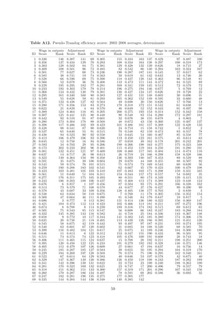
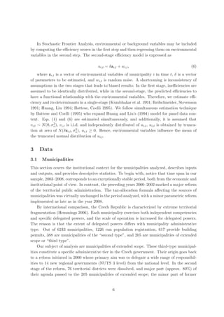
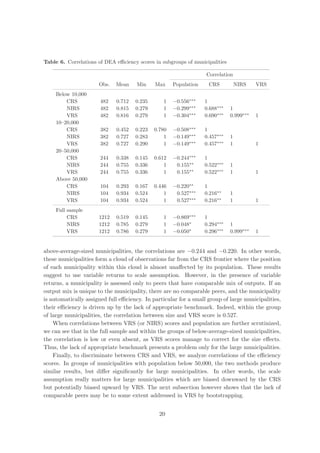
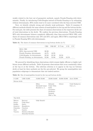
5. yi = f (xi ) + i , i = vi + u i . (1)
In contrast to DEA, a deviation from the frontier is not interpreted entirely as an inef-
ficiency. The statistical error i is rather decomposed into noise vi which is assumed to be
2
i.i.d., vi ∼ N (0, σv ), and a non-negative inefficiency term ui having usually half-normal or
truncated normal distribution.1 It is also assumed that cov(ui , vi ) = 0 and ui and vi are
independent of the regressors.
The Cobb-Douglas functional form for the costs writes
P
ln y = β0 + βp ln xp , (2)
p=1
while Translog generalizes Cobb-Douglas form by adding cross-products,
P P P
1
ln y = β0 + βp ln xp + βpq ln xp ln xq . (3)
2
p=1 p=1 q=1
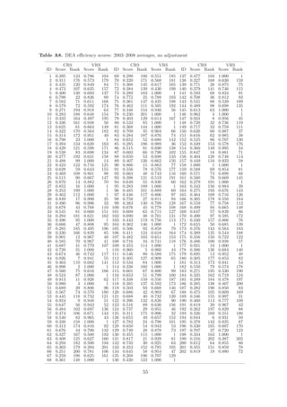
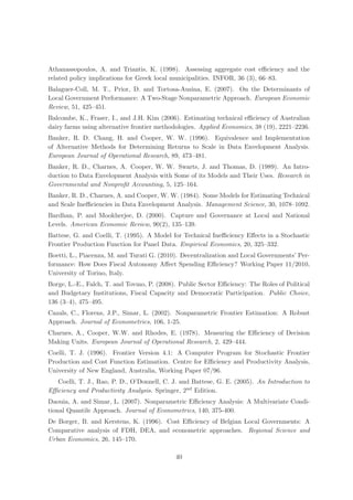
Battese and Coeli (1992) extend the original cross-sectional version of SFA in Eq. (1) to
panel data. The model is expressed as
yi,t = f (xi,t ) + i,t i,t = vi,t + ui,t , (4)
where yi,t denotes costs of municipality i in time t = T, T + 1, . . . and xi,t is vector of
2
outputs of municipality i in time t. Statistical noise is assumed to be i.i.d., vi,t ∼ N (0, σv ),
and independent of ui,t . Technical efficiency ui,t may vary over time
ui,t = ui exp[η(t − T )], (5)
where η is parameter to be estimated, and ui,t is assumed to be i.i.d. as truncations of
zero of N (µ, σu ). The model is estimated by maximum likelihood.2 Like Battese and Corra
2
2 2 2
(1977), we introduce parameter γ := σu /(σu +σv ) that conveniently represents the magnitude
of technical efficiency in the error term; if γ = 0, then all deviations from the frontier are
due to noise, while γ = 1 represents the opposite case when all deviations are attributed to
technical inefficiency.
1
Exponential or gamma distributions are chosen less commonly, and the resulting ranking is moreover
argued to be quite robust to the choice of the distribution (Coelli et al. 2005).
2
SFA estimation relies on decomposing observable i,t into its two components which is based on considering
the expected value of ui,t conditional upon i,t . Jondrow et al. (1992) derive the conditional distribution (half-
normal) and under this formulation, the expected mean value of inefficiency is:
σλ φ( i λ/σ) iλ
E[ui | i ] = − ,
1 + λ2 Φ(− i λ/σ) σ
where λ = σu /σv , φ(·) and Φ(·) are, respectively, the probability density function and cumulative distribution
2
function of the standard normal distribution, f (u| ) is distributed as N + − γ, γσv . If λ → +∞, the de-
terministic frontier results (i.e., one-sided error component dominates the symmetric error component in the
determination of ). If λ → 0, there is no inefficiency in the disturbance, and the model can be efficiently
estimated by OLS.
5

6. In Stochastic Frontier Analysis, environmental or background variables may be included
by computing the efficiency scores in the first step and then regressing them on environmental
variables in the second step. The second-stage efficiency model is expressed as
ui,t = δzi,t + wi,t , (6)
where zi,t is a vector of environmental variables of municipality i in time t, δ is a vector
of parameters to be estimated, and wi,t is random noise. A shortcoming is inconsistency of
assumptions in the two stages that leads to biased results: In the first stage, inefficiencies are
assumed to be identically distributed, while in the second-stage, the predicted efficiencies to
have a functional relationship with the environmental variables. Therefore, we estimate effi-
ciency and its determinants in a single-stage (Kumbhakar et al. 1991; Reifschneider, Stevenson
1991; Huang, Liu 1994; Battese, Coelli 1995). We follow simultaneous estimation technique
by Battese and Coelli (1995) who expand Huang and Liu’s (1994) model for panel data con-
text. Eqs. (4) and (6) are estimated simultaneously, and additionally, it is assumed that
2
vi,t ∼ N (0, σv ), vi,t is i.i.d. and independently distributed of ui,t , ui,t is obtained by trunca-
2
tion at zero of N (δzi,t , σu ), ui,t ≥ 0. Hence, environmental variables influence the mean of
the truncated normal distribution of ui,t .
3 Data
3.1 Municipalities
This section covers the institutional context for the municipalities analyzed, describes inputs
and outputs, and provides descriptive statistics. To begin with, notice that time span in our
sample, 2003–2008, corresponds to an exceptionally stable period, both from the economic and
institutional point of view. In contrast, the preceding years 2000–2002 marked a major reform
of the territorial public administration. The tax-allocation formula affecting the sources of
municipalities was virtually unchanged in the period analyzed, with a minor parametric reform
implemented as late as in the year 2008.
By international comparison, the Czech Republic is characterized by extreme territorial
fragmentation (Hemmings 2006). Each municipality exercises both independent competencies
and specific delegated powers, and the scale of operation is increased for delegated powers.
The reason is that the extent of delegated powers differs with municipality administrative
type. Out of 6243 municipalities, 1226 run population registration, 617 provide building
permits, 388 are municipalities of the “second type”, and 205 are municipalities of extended
scope or “third type”.
Our subject of analysis are municipalities of extended scope. These third-type municipal-
ities constitute a specific administrative tier in the Czech government. Their origin goes back
to a reform initiated in 2000 whose primary aim was to delegate a wide range of responsibil-
ities to 14 new regional governments (NUTS 3 level) from the national level. In the second
stage of the reform, 76 territorial districts were dissolved, and major part (approx. 80%) of
their agenda passed to the 205 municipalities of extended scope; the minor part of former
6

7. district services rests now with the 14 regions.3
Each municipality of extended scope administers a district comprising, on average, 30
other municipalities. Nevertheless, the third-type municipality always consists of the central
town in the district,4 so population of municipality of extended scope constitutes a relatively
large share of total population in the district; mean size of population in the municipality of
extended scope is 19,497 and mean population size of the district is 40,712.
Independent competencies of a municipality include provision of primary schools and
kindergartens, primary health care, local police, fire brigade, public utilities, territorial plan-
ning, maintenance of local roads, and garbage collection. Delegated responsibilities of the
municipalities of extended scope encompass mainly administration of population register, is-
suance of identity cards, travel documents, driving licenses, water and waste management,
environmental protection, management of forestry, local transportation provision, roads main-
tenance, social benefits payments, and social care services. The large extent of delegated
responsibilities is one of the motives for input-oriented analysis. However, in some fields,
the room for discretion is negligible not only on the output side, but also on the input side.
Especially for mandatory social transfers, the municipality is only an administrative interme-
diary disbursing funds allocated by the central government to beneficiaries. In the subsequent
subsection, we attempt to isolate away non-discretionary inputs and outputs.
The revenues of municipalities consist of tax revenues (in 2008, 44%), non-tax revenues
(11%), capital incomes (7%) and subsidies/grants (38%). Most of the tax revenue is via a
formula-based allocation of personal income tax, corporate income tax and value-added tax.
The allocation is a per-capita payment based on population size with 17 brackets (until 2008).
In municipalities, a small share of the total tax allocation is based on local incomes of the
self employed and the employed. In addition, there is some leeway for local revenue through
real-estate taxes (though within statutory limits) and fees. Grants are generally earmarked,
and a non-earmarked grant is also provided to cover the cost of providing central-government
services. There is regulation on debt, and revenues are also raised through sales of assets and
flows from off-budget accounts (Hemmings 2006).
Homogeneity is definitely key in efficiency estimation. In some within-country studies
(Afonso, Fernandez 2008), concern for homogeneity motivated even clustering district into
subsamples. Even though we can identify and isolate away outliers and also control for de-
terminants, a sufficiently homogeneous sample of municipalities is still necessary to eliminate
the risk of omitted variable bias and the resulting misspecification. Therefore, we opt for
municipalities with the extended powers: the range of responsibilities is similar, the districts
administered are of a similar size, the municipalities constitute regional centers, and the sam-
ple is large enough even for single-year cross-sectional analysis. In addition, the municipalities
of extended scope have much more discretion over spending than regions. Untied municipal
revenue in the form of tax and capital revenue accounts for over 70% of revenue, with ear-
marked grants accounting for the remainder. In contrast, a little under 40% of revenues of
3
The transfer of agenda from the former districts also explains why some statistics are still being collected
and provided only at the level of the non-existent administrative districts.
4
Figure A1 in Appendix shows geographical division of the Czech Republic into the districts administered
by the municipalities of extended scope.
7

8. the regional governments are untied (Hemmings 2006).
For the purpose of homogeneity, we exclude the capital city of Prague, which is not only
extremely large (with 1.2 milion inhabitants, four times the second largest city), but also
constitutes one of the 14 regions of the Czech Republic, hence exercises an idiosyncratic mix
of public services. From the sample, we eliminate also three other largest cities in the Czech
Republic, i.e., Brno (371,000), Ostrava (308,000) and Plzen (170,000). They substantially
exceed levels of population in the rest of the sample, where median is 12,212, mean is 19,497,
and maximal size is 101,268. The analysis is thus employed for 202 municipalities of extended
scope with population ranging from around 3,000 up to 101,000. The full list of municipalities
is provided in Table A1 in the Appendix.
3.2 Inputs
The crucial task in the computation of efficiency is to properly define outputs and inputs.
Following the majority of the literature (see six of out eight recent studies in Table A2),
we approximate inputs by Total current spending. This is even more appropriate given that
capital spending is highly volatile and subject to co-financing with EU Structural Funds. Our
source is the complete database of municipality budgets ARIS provided by the Ministry of
Finance.5 In the year 2008, the current expenditures represented 78% of total expenditures
(if mandatory expenditures were included) and 72% of total in the absence of mandatory
expenditures.
To provide a look into the budget composition, we aggregated data on current expenditures
into 10 groups: Administration; Agriculture; Culture and sports; Education; Environment
protection; Health; Housing and regional development; Industry and infrastructure; Public
safety; Social and labor market policy. Table 1 provides summary statistics of individual
expenditure groups. We excluded two groups of large mandatory payments: social transfers
payments and subsidies on education. The former are purely non-discretionary formula-
allocated grants that are earmarked and monitored in use, and the latter are temporary
transfers to municipalities in years 2003 and 2004 associated with financing of the primary
schools.6 The last column in Table 1 shows the share of each expenditure group in the average
budget after the exclusion. Prices are adjusted by CPI inflation and expressed in base year
2003.
5
Available at: http://www.mfcr.cz/cps/rde/xchg/mfcr/hs.xsl/aris.html
6
Since the year 2005, the state subsidies to primary schools are directly transferred to schools without
involvement of the municipality budgets.
8

9. Table 1. Expenditures: summary statistics
Mean Min Max Share (%)
Administration 73,782 18,608 413,069 32.06
Agriculture 1,604 0 34,134 0.7
Culture and sports 29,433 0 282,169 12.79
Education: discretionary 24,410 2,802 156,127 10.61
Environmental protection 20,246 0 175,700 8.80
Health 2,663 0 62,300 1.16
Housing and regional development 31,320 722 219,797 13.61
Industry and infrastructure 27,177 0 385,696 11.81
Public safety 9,719 0 122,909 4.22
Social care: discretionary 9,860 0 107,973 4.29
Total after exclusion 230,163 36,451 1,498,326 100.00
Source: ARIS database, Ministry of Finance; own calculations.
Note: Thousands (Czech koruna), N =1212.
To account for diverse cost conditions in municipalities, we alternatively work with the
wage-adjusted inputs. Thereby, we assume that the labor cost difference across regions may
serve as a good proxy for the overall cost difference. Wage adjustment input is particularly
useful in DEA where alternative ways to include wage in the production process are less
convenient. The wage variable nevertheless contains sizeable imperfections: since data on
gross wages are unavailable on the municipal level, we first collect wages for the 76 territo-
rial districts for the period 2003–2005, and in 2006–2008 use wage growth in 14 regions to
approximate for the district wages.
3.3 Outputs
Our preference for a comprehensive approach to efficiency is motivated by issues of fungibility
of spending and misclassifications into expenditure categories. Moreover, we can swiftly
disregard that some expenditure items may relate to various classes of outputs. At the same
time, a single output variable may be relevant for different classes of outputs. Our variable
selection is driven primarily by literature in the field (see Table A2 in the Appendix), by
the country specifics of the local public sector in the Czech Republic, data availability, and
by the attempt to match each specific expenditure group with a group-specific set of output
variables. As agriculture and health spending is negligible in municipalities budgets, we do
not seek outputs specific to these expenditure groups. In the end, we select the following 19
output variables, listed also in Table 2.
Administration Administration expenditures are related to size of Population of the dis-
trict administered by the municipality. This reflects that a municipality with extended powers
carries out many administrative services for the district as the whole. Social care expenditures
reflect support for retirements homes and homes for disabled, hence we include Old population
(population above 65 years of age) and the number of Homes for disabled among outputs.
9

10. Cultural facilities Expenditures on culture and sports comprise subsidies for theaters,
municipal museums and galleries, libraries, sport clubs, sport events and costs on monu-
ments preservation. The numbers of theaters, cinemas, children’s centers and libraries are all
summed into a variable of Cultural facilities; the facilities may be both private and public.
Additionally, we include the number of Municipal museums and galleries (hence, in pub-
lic ownership only), the number of Objects in municipal monuments reserve and the size of
Sporting and recreational area.
Education Municipalities finance mostly primary schools and kindergartens, while gram-
mar schools are financed mostly by the regional government. As a quantitative output, we
include the number of Pupils in primary schools and kindergartens in a municipality. To
evaluate the quality of education, we include the percentage of Pupils who enter the upper
secondary schools at the age of 11 or 13. Thereby, we exploit that children with higher skills
and better education have an option to enrol for a six-year or eight-year program in the upper
secondary schools with more demanding classwork.
Environment Environmental protection primarily deals with waste collection, air, soil and
ground water protection, and nature preservation. Municipal waste corresponds to expendi-
tures on waste collection. Pollution area is a variable that includes environmentally harming
areas such as built-up area and arable land, Nature reserves is linked to spending on nature
preservations, and the size of Urban green areas reflects spending on parks maintenance.
Housing and industry For housing and regional development we selected Built-up area
and the number of New dwellings completed. The built-up area corresponds to the extra pro-
vision of services of municipal utilities and the new dwellings represent the effect of municipal
financial support for housing construction. Industry and infrastructure spending contains
support of businesses, costs on municipal roads maintenance, support of public transporta-
tion and costs of water resources management. As corresponding outputs we use the number
of Businesses, the size of Municipal roads (close to traditionally measured surface of roads)
and the number of Bus stations.
Public safety Expenditures on public safety involve municipal police and fire brigade ser-
vices which we proxy by Built-up area served and Municipal police dummy.
10

11. Table 2. Outputs: summary statistics
Mean Min Max Source
Pupils in primary schools and kindergartens 2,154 81.96 11,944 IIE
Pupils entering secondary schools (%) 11.31 0 33.70 IIE
Cultural facilities 11.43 1 69 CZSO
Municipal museums and galleries 0.41 0 3 MGA
Objects in monuments reserve 25.83 0 254 NIM
Sporting and recreational area (ha) 35.12 2.35 273.6 CZSO
Municipal waste (tons) 14,942 16.19 124,836 ME
Nature reserves 10.67 0 48 ANCLP
Pollution area (ha) 2281 14.75 8,746 CZSO
Urban green area (ha) 51.37 3.09 351.7 CZSO
Built-up area (ha) 156.9 17.57 726.0 CZSO
New dwellings 39.47 0 600 CZSO
Businesses 4,440 521 33,084 CZSO
Municipal roads (ha) 52.85 6.62 202.6 CZSO
Bus stations 30.71 4 112 IDOS
Population in district 40,712 9,175 160,720 CZSO
Old population 2,744 380 17,297 CZSO
Homes for disabled 0.41 0 4 CZSO
Municipal police 0.87 0 1 CZSO
Sources: ANCLP = Agency for Nature Conservation and Landscape Protection, MGA = Museums
and Galleries Association, CZSO = Czech Statistical Office, IDOS = Transportation timetables, IIE
= Institute for Information on Education, ME = Ministry of Environment, NIM= National Institute
of Monuments.
Note: N = 1212.
As a very preliminary analysis, we carry out individual pre-analyses for each expenditure
group, shown in Table 3. In simple pooled OLS, we regress the group-relevant outputs on
group expenditures and realize that R2 falls within the range 0.70–0.90 in all but two cases; for
Housing and Social care, we cannot find better outputs to increase R2 above 0.45. Although
the variable of municipal museums and galleries has negative significant coefficient, we keep
it among outputs. Small municipalities, i.e. those having lower spending, are more likely to
have municipal museums than big municipalities, where many private museums and galleries
operate and survive more easily. Similarly, we observe negative coefficient for new dwellings
which may reflect some specific characteristic of a municipality where housing construction is
more developed, hence we also keep it among outputs.
When selecting outputs, we also consider tradeoff between relevance and dimensionality.
Irrelevant outputs can bias efficiency scores but a high number of (especially highly correlated)
outputs artificially makes many municipalities fully efficient. In addition, efficiency analysis
suffers from misspecification if the model omits relevant variables or if it includes irrelevant
variables. Omission of relevant variables leads to underestimation of the mean efficiency,
11

12. Table 3. Outputs relevant for the individual expenditure groups (pooled OLS)
Education Housing
Constant −582.7 Constant −688.2
∗∗∗ ∗∗∗
Pupils in primary schools and kindergartens 11.36 Built-up area 218.6
∗ ∗∗∗
Pupils entering secondary schools 94.84 New dwellings −39.6
R2 0.902 R2 0.438
Culture Environment
∗∗∗ ∗∗∗
Constant −3,446 Constant −8,820
∗∗∗ ∗∗∗
Cultural facilities 2,587 Municipal waste 0.727
∗∗∗ ∗∗∗
Municipal museums and galleries −7,334 Nature reserves 275.5
∗∗∗ ∗∗∗
Objects in monuments reserve 66.24 Pollution area 3.617
∗∗∗ ∗∗∗
Sporting and recreational area 162.8 Urban green area 149.3
R2 0.731 R2 0.785
Industry and infrastructure Public safety
∗∗∗ ∗∗∗
Constant −16,088 Constant −6,693
∗∗∗ ∗∗∗
Businesses 8.962 Built-up area 87.29
∗ ∗∗∗
Municipal roads 33.62 Municipal police 3,372
∗∗
Bus stations 77.52
R2 0.880 R2 0.700
Administration Social care
∗∗∗
Constant 1,120 Constant 1,665
∗∗∗ ∗∗∗
Population in district 1.807 Old population 2.507
∗∗∗
Homes for disabled 2,496
2
R 0.818 R2 0.402
while the inclusion of irrelevant variables leads to overestimation, and the effect of omission
of relevant inputs on efficiency is more adverse compared to the inclusion of irrelevant ones
(Galagedera, Silvapulle 2003).
If we err on the side of caution and include a larger set of outputs, the problem of di-
mensionality emerges. As a given set of observations is projected in an increasing number
of orthogonal directions, the Euclidean distance between the observations necessarily must
increase. Moreover, for a given sample size, increasing the number of dimensions results in
more observations lying on the boundaries of the estimated production set (Simar, Wilson
2008). When dimensionality is large, unless a very large quantity of data is available, the
results will have a large bias, large variance and very wide confidence intervals.
Banker et al. (1989) argues that the total number of observations should be at least three
times as much as the total number of inputs and outputs. Additional tests show that the ratio
of observations and dimensionality should be even higher (Pedraja-Chaparro et al. 1999). On
the basis of convergence rates for DEA estimators, Simar and Wilson (2008) also conclude that
a much larger sample size is needed. In our case, we would have 202 (or 1212) observations
and 20 inputs and outputs in total, therefore some reduction is reasonable.
12

13. The recent literature offers several methods how to decrease dimensionality. Geys and
Moesen (2009a) seek the most representative output per each expenditure group and con-
struct the set of outputs from a few pre-selected variables. Borge et al. (2008) apply fixed
national cost weights upon 20 indicators; Afonso and Fernandez (2008) normalize to aver-
ages. Most often, however, discrimination among outputs tends to diminish importance of
outputs that are largely correlated with others. Two procedures stand out in the literature.
Jenkins and Anderson (2003) propose a variable-reduction procedure that decides which of
the original correlated variables can be entirely omitted with the least loss of information.
In contrast, principal component analysis decreases dimensionality by produces uncorrelated
linear combinations of the original outputs. Adler and Yazhemsky (2010) apply Monte Carlo
simulation to generalize that principal components analysis provides a more powerful tool
with consistently more accurate results. Adler and Yazhemsky (2010) also suggest that the
most cautious approach would be to drop PCs one-by-one until a reasonable level of discrim-
ination is achieved or until you have reached the rule-of-thumb of at least 80% (or 76% under
VRS) of the variance of the original data.
If we included all output variables as outputs, the model would have 20 (19+1) dimensions.
This dimensionality would not only bring wide confidence intervals, but is also unnecessary, as
many variables contain largely identical information related to the municipality size. Table A4
shows the correlation matrix of output variables, where population of a municipality is very
highly correlated with the number of pupils (0.993), the number of old people (0.988), the
number of businesses (0.967), built-up area (0.935), the length of municipal roads (0.916),
district population (0.898), municipal waste (0.846), cultural facilities (0.831), and urban
green area (0.827).
Therefore, we follow principal components analysis and use the 80-percent rule. Table 4
shows weights of the output variables that are aggregated into the first six principal compo-
nents. Six components suffice to explain 80.28% of the variance in the original outputs. The
first component PC1 explains more than 51.6% of the variance and represents the size effect
of a municipality, as it mainly contains information of variables which are highly correlated
with population; note that correlation between population in the municipality and PC1 is
0.976. PC2 represents mostly cultural outputs, PC3 is for environmental amenities, PC4 is
quality of educating and raising children, and PC5 is safety. For some observations, the values
of components can be negative.
To get positive output data, we apply an affine transformation which does not affect results
either for SFA or DEA (Ali, Seiford 1990; Pastor 1996). Specifically, for each municipality
i, we transform the original value of a component k, Yk,i , ∀k ∈ {1, . . . , 6}. We obtain the
transformed value Yk,i = Yk,i + Bk , where Bk = | min{Yk,i }N | + 1 which will ensure strictly
i=1
positive output data.
In the next step, we try to identify atypical observations which can be outliers and therefore
distort our efficiency estimates. Outliers play a relatively important role in determining
efficiency scores of other observations in the sample. By distorting efficiency frontier, some
virtually efficient observations may be regarded as inefficient. To obtain robust scores, it is
thus necessary to identify and potentially remove the outliers. Out of several ways how to
13

14. Table 4. Principal component analysis
PC1 PC2 PC3 PC4 PC5 PC6
Eigenvalue 9.799 1.385 1.280 1.089 0.906 0.795
Proportion 0.516 0.073 0.067 0.057 0.048 0.042
Cumulative 0.516 0.589 0.656 0.713 0.761 0.803
Pupils in primary schools and kindergartens 0.308 -0.126 -0.040 0.041 -0.004 0.021
Pupils entering the upper secondary schools -0.041 0.292 0.149 0.615 -0.559 -0.297
Cultural facilities 0.272 0.076 -0.130 0.033 -0.034 0.093
Municipal museums and galleries -0.070 0.339 -0.471 0.332 0.227 0.579
Objects in monuments reserve 0.132 0.546 0.253 -0.076 -0.028 0.135
Sport in and recreational area 0.203 0.283 -0.024 -0.133 0.210 -0.407
Municipal waste 0.269 -0.171 -0.045 0.088 -0.100 0.084
Nature reserves 0.079 0.141 0.648 -0.212 0.166 0.292
Pollute area 0.219 0.361 -0.237 -0.184 0.097 -0.158
Urban green area 0.256 -0.169 -0.111 0.012 0.077 -0.232
Built-up area 0.305 0.002 -0.036 0.014 -0.042 0.041
New dwellings 0.217 0.139 0.140 -0.052 -0.346 0.179
Businesses 0.308 -0.064 0.015 0.037 -0.083 0.047
Municipal roads 0.251 0.218 -0.209 -0.110 0.111 -0.219
Bus stations 0.241 -0.151 -0.025 0.159 -0.071 0.296
Population in district 0.288 -0.107 0.171 0.002 0.007 0.125
Old population 0.311 -0.079 -0.024 0.029 -0.072 0.021
Homes for disabled 0.179 -0.286 0.015 0.136 0.061 -0.015
Municipal police 0.079 0.003 0.296 0.581 0.619 -0.158
14

15. deal with outliers, we apply both Wilson’s method (Wilson 1993) and order-m frontiers by
Cazals et al. (2002). A full description of the methods follows in Section A.2 in Appendix.
Firstly, we estimate Wilson statistics (Wilson 1993) to observe maximally 10 potential
outliers for each year. We construct log-ratio plot of the statistics and define from 5 to
10 potential outliers with only small variance across years. When closely scrutinized, we
find out that all of them are bigger cities representing regional centers with atypically high
outputs. We decide to keep these data in the sample, as there are no errors in the data
and these observations are atypical only because of size. We also perform an additional test
for outlier detection based on order-m frontiers (Czasals et al. 2002) that scrutinizes super-
efficient observations. We construct order-m efficiency scores for m = 25, 50, 100, 150, and
find no super-efficient observation with a low DEA score, hence our super-efficient values do
not distort efficiency rankings.
3.4 Determinants
The idea to test for effects of various demographic, economic and political variables upon
efficiency scores. The determinants may represent either (i) a direct effect of operational
environment on pure inefficiency (either technical or allocative), or the presence of (ii) non-
discretionary inputs and (iii) unobservable outputs. Non-discretionary inputs represent pro-
duction in a more or less favorable environment, e.g., stocks of human capital and other
competitiveness indicators. Unobservable outputs are typically associated with service qual-
ity; given that we focus on core services with largely quantitative characteristics, extra value
added of services may be produced based on the characteristics of the municipalities, such as
the municipality size and the level of income. We cannot neglect the hidden inputs or out-
puts; once the selection of inputs and outputs is imperfect, missing inputs and extra outputs
may be misinterpreted as budgetary slack in terms of low effort, over-employment and large
private rents.
Unfortunately, a single determinant may theoretically bring in several effects, and extra
analysis is required to discriminate between the effects. Moreover, there is vague bound-
ary between the very definition of the effects. For instance, explaining inefficiency by slack
stemming from less effort can be alternatively interpreted as lower amount of human capital,
which is not slack, but lacking input. Sometimes, like in the case of education variable, we
can suspect the presence of hidden inputs and hidden outputs at the same time, where each
predicts the opposite sign of the education variable. Thus, our interest is restricted mainly
to finding if the overall effect is robust across specifications, and based on the sign we may
conclude which of the effects dominates.
In line with the literature, and based on the data available, we control for the following
determinants:
Population Economies of scale and agglomeration externalities typically make the larger
municipalities more efficient; moreover, small governments are less efficient than the central
government due to fiscal vulnerability, or the absence of sufficient experience among local
staff (Prud’homme 1995). Small governments may also be captured by local interest groups
15

16. (Bardhan, Mookherjee 2000), or prone to moral hazard if dependent on transfers from the
central government (Rodden 2003). On the other hand, higher electoral control typical at the
local level reduces incentives for incumbents for rent-seeking (Seabright 1996) and yardstick
competition disciplines local representatives not to waste resources. In addition, the scale
economies and agglomeration externalities may be larger in the private than public sector,
hence the relative cost of public sector (e.g., reservation wage) increases in a large municipality.
We introduce dummies for population sizes of the municipalities around three thresholds:
10,000; 20,000 and 50,000. This construction reflects that population variable as such is
highly correlated with the first component. Another point is that the three thresholds are
also used in tax-revenue sharing schemes, consisting of 17 population thresholds in total.
Geography The smaller is geographical distance between the municipality and the regional
center, the higher is (yardstick) competition between municipalities, and also more direct
access to local public goods provided by the region. Both yardstick competition and the level
of consumption spillovers suggest that distance increases costs hence reduces input-oriented
efficiency; evidence for the effect is, inter alia, in Loikkanen and Susiluoto (2005). We measure
distance in time to reach the regional center; for municipalities located in the center, we
measure distance to the closest neighboring regional center. The spatial interdependence
between efficiency scores can also be analyzed in the direct way, but based on the preliminary
ˇt
spatial analysis of groups of expenditures (Sˇastn´ 2009), we leave this topic to future research.
a
Education Municipalities with a higher share of University graduates may be more efficient
either by disposing with more qualified labor, or through voters’ higher and more competent
control (De Borger, Kerstens 1996). Yet, university graduates may also raise productivity in
the private sector, and raise reservation wage for the public sector. In addition, wealth or
income effect cannot be identified directly, and education thus may involve also the income
effect that leads to demand for (unobservable) high-quality services. The effect of education
is thus ambiguous. We are also aware of reverse causality; the characteristics that make a
municipality cost-efficient may also attract the mobile (high-skilled) citizens. A good message
is at least that correlation of the variable with the output variable Pupils entering secondary
schools is only 0.027, hence the effect of graduate education is not captured in the output
variable. This point is particularly relevant in the Czech context where the parent’s education
is the strongest determinant of a pupil’s achievement.
Fiscal capacity Low fiscal capacity may serve as a hard-budget constraint that reduces
public sector wages, lowers operating surpluses and induces fiscal stress, in which case effi-
ciency goes up. This finding is in line with earlier analyses of overall efficiency in Belgium
(De Borger et al. 1994; De Borger and Kerstens 1996), and Spain (Balaguer-Coll et al. 2007).
We introduce three dimensions of fiscal capacity. The extent how municipality is depen-
dent on Self-generated revenues is the direct measure of hard-budget constraint. Balaguer-Coll
et al. (2007) speak in this case of “patrimonial revenues” and relate them to lower willing-
ness to save. Next, we study whether the past Government debt implying larger interest and
16

17. amortization payments serve as fiscal hardship that improves efficiency. Geys and Moesen
(2009a) find that high debt repayments rather impinges on municipal efficiency; the idea is
that past fiscal mismanagement persists over time. The last fiscal variable is Capital spending.
A hypothesis is that fiscal vulnerability, in this case high capital investment in a given year,
pushes for cost savings on the current expenditures (Athanassopoulos, Triantis 1998).
By including Subsidies from the upper levels of government among determinants, we an-
swer the question whether the grants fully translate into a larger provision of public goods or
if municipalities receiving higher grants tend to be less efficient (Hines, Thaler 1995). Em-
pirical evidence supports that the option of sharing expenditures in a broader constituency
induces slack, hence the “flypaper effect” is rather significant (e.g. Kalb 2010; De Borger et
al. 1994; De Borger, Kerstens 1996; Loikkanen, Susiluoto 2005).
Politics Political characteristics of a municipality may largely influence its efficiency. By
weak-government hypothesis, high Political concentration reflecting low party fragmentation
should decrease narrowly focused spending, hence should improve efficiency. Some evidence
nevertheless suggests that single-party municipal governments in particular are inefficient
(Geys et al. 2010; Borge et al. 2008). In Czech municipalities, concentration could be measured
either in the council or in the executive board led by the mayor. The members of the executive
board, including the mayor and the deputy mayor, are elected from the members of the local
council and represent the majority coalition. We dispose only with data on seats in the
municipality council, hence our concentration index (i.e., Laakso-Taagepera or Hirschmann-
Herfindahl index) exhibits downward bias relative to concentration of the executive power in
the coalition.
Electoral year may be related to larger spending into additional (unobservable) outputs,
hence to inefficiency. At the same time, local elections take place in the same year like national
election, hence effects are confounded with the national political business cycle. Wage growth
in the electoral year is nevertheless average, namely third largest in the sample out of six
years.
Additionally, we consider political ideology, albeit it is not easy to identify ideology on
the local level. We prefer to measure the share of municipal-council representatives from
Left-wing parliamentary parties (Social Democrats and Communists) out of representatives
from all parliamentary parties. Geys et al. (2010) find that the high share of left-wing parties
is associated with higher efficiency. We expect the opposite; the left-wing parties in the Czech
Republic have an older and less educated electorate, and this should represent less monitoring
and higher level of the social services, which are in our dataset unobservable output variables.
Moreover, ideological variable may also represent (un)willingness to introduce high-powered
incentives in the public sector.
Finally, we include two variables that are related to the interest in monitoring and shap-
ing local politics. The first is the share of seats of Parliamentary parties in the municipality
council. The second is voters’ involvement measured by Turnout in municipal elections (see
Geys et al. 2010; Borge et al. 2008). While the former is expected to increase costs, the latter
should improve efficiency.
17

18. Table 5 presents statistics of potential determinants; more information about the data
follows in Table A5 in the Appendix. Correlation matrix of the determinants in Table A6
features generally very low degrees of correlation. Only two patterns stand out. In small mu-
nicipalities (below 10,000 inhabitants), we find less university-educated people (−0.378), less
votes for parliamentary hence more votes for local parties (−0.331) and bigger voters’ turnout
(0.661). In contrast, large municipalities (above 50,000 inhabitants) attract better educated
citizens (0.385), lead to more concentrated political competition (0.233) of parliamentary
rather then local parties (0.197), and local elections have lower turnout (−0.395).
Table 5. Determinants: descriptive statistics
Mean Std. Dev. Min Max
Pop < 10,000 0.398 0.490 0 1
Pop 10,000–20,000 0.315 0.465 0 1
Pop > 50,000 0.086 0.280 0 1
University graduates (%) 6.154 1.589 2.540 12.20
Subsidies per capita 3,856.3 3,451.8 73 25,511
Capital expenditures per capita 5,473.2 3,293.6 481 37,567
Lagged debt dummy 0.446 0.497 0 1
Self-generated revenues (%) 18.06 5.534 6.39 43.77
Distance from regional center 37.84 16.40 11 101
Voters’ turnout 42.38 7.413 21.69 60.55
Political concentration 0.218 0.053 0.107 0.539
Left-wing share 0.447 0.127 0 1
Parliamentary parties (%) 0.721 0.156 0.220 1
Electoral year dummy 0.167 0.373 0 1
Source: Czech Statistical Office, Ministry of Finance.
Note: N = 1212. Nominal data adjusted for inflation, base year 2003.
4 Non-parametric efficiency
4.1 General results
This section presents cross-sectional results computed by Data Envelopment Analysis in the
years 2003–2008. We allow for constant (CRS), variable (VRS) and non-increasing returns to
scale (NIRS). Figure 1 presents the distributions of efficiency scores where we average year-
specific municipality scores over the 2003–2008 period. As outputs do not vary too much over
time, averaging scores computed for each year can smooth errors on the input side. Unlike
the upper three panels, the bottom three panels in Figure 1 adjust for wage differences.
The distribution of CRS scores substantially differs from that of VRS and NIRS. On the
other hand, distributions of VRS and NIRS scores are very similar, hence municipalities very
rarely operate on the part of production function with increasing returns to scale. Wage
adjustment does not introduce major differences in either case; the distributions with adjust-
18

19. 15
20
20
15
15
10
Percent
Percent
Percent
10
10
5
5
5
0
0
0
.2 .4 .6 .8 1 .4 .6 .8 1 .4 .6 .8 1
(a) CRS (b) VRS (c) NIRS
15
25
20
20
15
10
15
Percent
Percent
Percent
10
10
5
5
5
0
0
0
.2 .4 .6 .8 1 .4 .6 .8 1 .4 .6 .8 1
(d) CRS, adjustment (e) VRS, adjustment (f) NIRS, adjustment
Figure 1. Distributions of DEA efficiency scores: 2003–2008 averages
ment are only a bit smoother suggesting that some extreme efficiency scores can be attributed
to relatively (un)favorable wage conditions in the municipality.
Concerning the case without adjustment, the mean value of CRS score is 0.52 and mini-
mum is 0.22. There is only single observation which is fully efficient under CRS for the whole
period. For VRS, both mean value (0.79 > 0.52) and minimum (0.39 > 0.22) increase, as
by construction of the VRS frontier, the observations are closer to the VRS frontier. The
amount of fully efficient municipalities under VRS varies from 52 in 2005 to 61 in 2007 and
there are 30 municipalities which stay fully efficient over the whole period. The Appendix
offers descriptive statistics for individual years (Table A7), individual CRS and VRS averaged
scores in the case without adjustment (Table A8) and with adjustment for wage differences
(Table A9).
4.2 Population subgroups
To obtain a further insight into the differences of efficiency scores under different scale assump-
tions, it may be useful to explore how these differences vary across subgroups of municipalities
defined by population size. Table 6 presents summary statistics and correlations for scores of
municipalities if divided into four groups. We use again 2003–2008 averages and the results
presented are without wage adjustment. The pattern of correlations is similar for the case
with wage adjustment.
CRS scores are highly correlated with the size of population levels if measured in the full
sample (−0.869). This only confirms the finding of VRS that large municipalities operate
on the part of production function with decreasing returns to scale. However, size is not
very indicative of efficiency if we look at within-group differences. For the two groups of
19

20. Table 6. Correlations of DEA efficiency scores in subgroups of municipalities
Correlation
Obs. Mean Min Max Population CRS NIRS VRS
Below 10,000
CRS 482 0.712 0.235 1 −0.556∗∗∗ 1
NIRS 482 0.815 0.279 1 −0.299∗∗∗ 0.688∗∗∗ 1
VRS 482 0.816 0.279 1 −0.304∗∗∗ 0.690∗∗∗ 0.999∗∗∗ 1
10–20,000
CRS 382 0.452 0.223 0.780 −0.508∗∗∗ 1
NIRS 382 0.727 0.283 1 −0.149∗∗∗ 0.457∗∗∗ 1
VRS 382 0.727 0.290 1 −0.149∗∗∗ 0.457∗∗∗ 1 1
20–50,000
CRS 244 0.338 0.145 0.612 −0.244∗∗∗ 1
NIRS 244 0.755 0.336 1 0.155∗∗ 0.522∗∗∗ 1
VRS 244 0.755 0.336 1 0.155∗∗ 0.522∗∗∗ 1 1
Above 50,000
CRS 104 0.293 0.167 0.446 −0.220∗∗ 1
NIRS 104 0.934 0.524 1 0.527∗∗∗ 0.216∗∗ 1
VRS 104 0.934 0.524 1 0.527∗∗∗ 0.216∗∗ 1 1
Full sample
CRS 1212 0.519 0.145 1 −0.869∗∗∗ 1
NIRS 1212 0.785 0.279 1 −0.048∗ 0.294∗∗∗ 1
VRS 1212 0.786 0.279 1 −0.050∗ 0.296∗∗∗ 0.999∗∗∗ 1
above-average-sized municipalities, the correlations are −0.244 and −0.220. In other words,
these municipalities form a cloud of observations far from the CRS frontier where the position
of each municipality within this cloud is almost unaffected by its population. These results
suggest to use variable returns to scale assumption. However, in the presence of variable
returns, a municipality is assessed only to peers that have comparable mix of outputs. If an
output mix is unique to the municipality, there are no comparable peers, and the municipality
is automatically assigned full efficiency. In particular for a small group of large municipalities,
their efficiency is driven up by the lack of appropriate benchmark. Indeed, within the group
of large municipalities, the correlation between size and VRS score is 0.527.
When correlations between VRS (or NIRS) scores and population are further scrutinized,
we can see that in the full sample and within the groups of below-average-sized municipalities,
the correlation is low or even absent, as VRS scores manage to correct for the size effects.
Thus, the lack of appropriate benchmark presents a problem only for the large municipalities.
Finally, to discriminate between CRS and VRS, we analyze correlations of the efficiency
scores. In groups of municipalities with population below 50,000, the two methods produce
similar results, but differ significantly for large municipalities. In other words, the scale
assumption really matters for large municipalities which are biased downward by the CRS
but potentially biased upward by VRS. The next subsection however shows that the lack of
comparable peers may be to some extent addressed in VRS by bootstrapping.
20

21. 4.3 Bias-corrected scores
Our next step is to bootstrap VRS efficiency scores to allow for statistical inference. The
original DEA scores are biased by construction (see Section A.3) and bootstrapping helps
us to correct for the bias and construct confidence intervals for each efficiency score. To
apply homogenous bootstrap as developed by Simar and Wilson (1998), the independence
assumption has to hold. For this purpose, we employ graphical test of independence developed
by Fisher and Switzer (1985) and described in Wilson (2003). The χ-plot for the VRS
efficiency scores in 2008 reveals that all observations are inside the required interval, hence
the independence assumption holds.7
We apply homogeneous bootstrap by an algorithm described in Simar and Wilson (1998)
with 2, 000 bootstrap replications. Figure 2 shows the distribution of bias-corrected effi-
ciency scores averaged over the period 2003–2008 compared to the original VRS estimates
and Table 7 offers summary statistics.8 The distribution of bias-corrected scores is denser
but otherwise has a very similar pattern as the original distribution. An expected change
is that the originally fully efficient municipalities are shifted to lower percentiles. Generally,
municipalities with the lack of comparable observations, i.e. large municipalities in our con-
text, have larger bias and wider confidence intervals. Hence, correction for bias does not help
us to deal effectively with the large municipalities. The decrease in efficiency scores of large
municipalities also explains why bias-corrected VRS scores correlate with CRS scores more
than the original VRS scores (cf. Table 8).
Table 7. VRS and bias-corrected VRS efficiency scores (2003–2008 averages): summary statistics
Mean Min Max
(a) VRS 0.786 0.387 1
(b) VRS, adjustment 0.784 0.385 1
(c) VRS, bias-corrected 0.694 0.364 0.879
(d) VRS, adjustment, bias-corrected 0.692 0.362 0.892
Figure 3 illustrates the size of confidence intervals of the bias-corrected VRS efficiency
scores averaged over 2003–2008 in the case without adjustment. (These correspond to Panel
(c) in Fig. 2.) The municipalities are ordered by their original VRS efficiency scores. Ap-
parently, the originally fully efficient observations have large confidence intervals. Yet, the
ranking of municipalities does not change substantially, as is expressed by the Spearman’s
correlation coefficients of 0.954 (no adjustment) and 0.949 (wage adjustment). Figure 3 also
helps to identify municipalities with atypical values of input-output combinations which have
wide intervals even for relatively small scores.
Table 8 summarizes the correlations between six alternative specifications for non-parametric
efficiency. We prefer the bias-corrected VRS specification with wage adjustment (denoted
7
Results of the test are available per request.
8
The analysis runs in R software with FEAR package (Wilson 2008). The detailed data on bias-corrected
efficiency scores are available in Table A10 in Appendix, and individual data on confidence intervals can be
provided upon request.
21

22. 25
20
20
15
15
Percent
Percent
10
10
5
5
0
0
.4 .6 .8 1 .4 .6 .8 1
(a) VRS (b) VRS, adjustment
25
20
20
15
15
Percent
Percent
10
10
5
5
0
0
.4 .5 .6 .7 .8 .9 .4 .5 .6 .7 .8 .9
(c) VRS, bias corrected (d) VRS, adjustment, bias corrected
Figure 2. Distributions of the original VRS and the bias-corrected VRS efficiency scores:
2003–2008 averages
1
0.9
0.8
0.7
0.6
0.5
0.4
0.3
Figure 3. Bias-corrected scores and their confidence intervals: 2003–2008 averages
VRS BC). For robustness check, it is nevertheless illustrative to observe two facts. First, the
presence or absence of wage adjustment does not change rankings substantially (correlations
0.98, 0.964, 0.93). Second, correlations between methods differing only in returns to scale
22

23. assumption are larger in the case with wage adjustment (0.345, 0.408, 0.95) than without
adjustment (0.296, 0.359, 0.949). This is another reason for incorporating relative wages in
the analysis.
Table 8. Spearman rank correlations of DEA efficiency scores
No adjustment Wage adjustment
CRS VRS VRS BC CRS VRS VRS BC
CRS 1
No adjustment VRS 0.296 1
VRS, bias-corr. (BC) 0.359 0.949 1
CRS 0.980 0.300 0.362 1
Wage
VRS 0.313 0.964 0.910 0.345 1
adjustment
VRS, bias-corr. (BC) 0.374 0.910 0.930 0.408 0.950 1
5 Parametric efficiency
5.1 Results without determinants
This section computes efficiency scores using Stochastic Frontier Analysis.9 Unlike DEA,
where year-specific scores are obtained only as cross-sectional estimates, SFA estimates the
time-profile of the scores endogenously in a single panel. In addition, determinants can be
conveniently included. We consider various specifications: Cobb-Douglas or a more flexible
Translog cost function, time-variant or time-invariant efficiency, and efficiency with determi-
nants and without determinants. Furthermore, we treat wage differentials in three ways: (i)
no adjustment, (ii) spending adjusted by wage differences exactly as in DEA, and (iii) wages
included directly into the cost function. Since wage differentials influence costs directly, we
disregard the option when the wage is a part of the vector of determinants. In total, we
cope with four dimensions of modeling. We first assess time variance, the inclusion of wage
differences, and then discuss the appropriate functional form. Finally, we examine the effect
of determinants.
Our baseline estimates for Cobb-Douglas production are in Table 9. First and foremost,
coefficients of principal components suggest that the components may be irrelevant explana-
tory variables. Albeit PC1 is always significant and positively affects total costs, most of
the other components have insignificant positive or even negative effect on costs. Our read-
ing is that either we have constructed irrelevant outputs or another functional specification
(Translog) is required. As expected, the wage positively affects costs. Concerning other
parameters, the variance of the inefficiency in total error variance is relatively large, and
statistical noise accounts only for 1 − γ ≈ 15% of the total variance. Significance of param-
eter µ confirms that assumption of truncated-normal distribution is more appropriate than
half-normal distribution.
9
We use software Frontier 4.1 developed by Coelli (1996) for parametric estimation.
23

24. Importantly, the parameter η is significant, so efficiency does change over time. In the
case without any wage variable, the parameter is negative and significant, which suggests that
efficiency decreases over time. Once we control for wages, the sign is exactly opposite, i.e. the
efficiency increases over time. Inclusion of wages in the panel data estimation is thus crucial
as the real wages increase over time and this effect translates into an increase in spending.
As a result, we abandon all time-invariant models that abstract away from wage differences.
Table 9. Baseline SFA results: Cobb-Douglas function, no determinants
No adjustment Wage in outputs Wage adjustment
TI TV TI TV TI TV
∗∗∗ ∗∗∗ ∗∗∗ ∗∗∗ ∗∗∗ ∗∗∗
β0 10.391 10.408 8.045 5.600 8.200 7.510
∗∗∗ ∗∗∗ ∗∗∗ ∗∗∗ ∗∗∗ ∗∗∗
PC1 1.164 1.161 1.144 1.135 1.042 1.061
∗∗∗ ∗∗∗ ∗∗∗ ∗∗∗ ∗∗∗ †
PC2 −0.169 −0.160 −0.151 −0.133 −0.163 −0.071
∗
PC3 0.000 0.013 0.008 −0.058 −0.112 −0.074
† †
PC4 0.049 0.038 0.048 0.040 −0.020 0.036
† †
PC5 −0.045 −0.037 0.000 −0.042 −0.026 −0.017
∗ ∗∗ ∗ ∗∗∗
PC6 −0.124 −0.149 −0.171 −0.140 −0.286 −0.061
∗∗∗ ∗∗∗
Wage 0.247 0.504
∗∗∗ ∗∗∗ ∗∗∗ ∗∗∗ ∗∗∗ ∗∗∗
σ2 0.077 0.079 0.064 0.074 0.096 0.081
∗∗∗ ∗∗∗ ∗∗∗ ∗∗∗ ∗∗∗ ∗∗∗
γ 0.858 0.858 0.834 0.855 0.875 0.861
∗∗∗ ∗∗∗ ∗∗∗ ∗∗∗ ∗∗∗ ∗∗∗
µ 0.515 0.520 0.462 0.504 0.579 0.529
∗ ∗∗∗ ∗∗∗
η −0.007 0.016 0.038
Log likelihood 648.8 652.7 655.0 667.2 560.4 656.7
∗∗∗
LR one-sided error 1136 1144 ∗∗∗ 1137 ∗∗∗ 1161 ∗∗∗ 1045 ∗∗∗ 1237 ∗∗∗
Note: ∗∗∗ , ∗∗ , ∗ denote statistical significance at 1%, 5% and 10% level, respectively. †
denotes statistical
significance at 10% level on one-tail.
In the next step, we estimate efficiency by means of Translog production with time-
variant efficiency and wage differences included. Table 10 reports the results. The first and
the third column include all cross-product terms of principal components, i.e. the number of
explanatory variables increases from 6 (7) to 27 (28). Some of the basic principal components
are still negative and their significance does not change much in comparison with the baseline
case. Most of the cross-product terms (16 out of 21) are not significant either. Hence,
we drop explanatory variables with high p-value and after a few iterations end up with a
new production function encompassing only four significant components and seven significant
cross-product terms. This Pseudo-Translog function is captured in the second and fourth
column of Table 10. Log-likelihood decreases only slightly when insignificant variables are
dropped out. Interestingly, all principal components are part of the new production function,
although some of them enter the production only in an interaction with another component.
Thus, we may conclude that components computed from our output variables are indeed
relevant for this analysis. Finally, the estimated parameters γ, µ and η are similar to those
obtained in baseline Cobb-Douglas specification with time-variance and wage differences.
Table A11 in the Appendix offers individual scores for the Pseudo-Translog, both with costs
adjusted by wage differences and wages in outputs.
24

25. Table 10. Modified SFA results: Translog and Pseudo-Translog production functions,
time-variant efficiency, no determinants
Wage in outputs Wage adjustment
Translog Pseudo-Translog Translog Pseudo-Translog
∗∗∗ ∗∗∗ ∗∗∗ ∗∗∗
β0 8.802 5.816 11.709 10.587
PC1 0.507 0.265
∗∗ ∗∗∗ ∗∗∗ ∗∗∗
PC2 −2.031 −0.903 −2.145 −1.808
† † ∗∗∗
PC3 −0.936 −0.215 −0.977 −0.390
†
PC4 −0.245 −0.199 −0.062
† ∗∗∗ † ∗∗∗
PC5 −1.087 −0.323 −1.151 −0.215
† † ∗∗
PC6 −1.208 −1.000 −0.992
∗∗∗ ∗∗∗
Wage 0.584 0.614
∗∗∗ ∗∗∗ ∗∗∗ ∗∗∗
PC11 0.439 0.471 0.553 0.555
∗∗∗
PC21 0.208 0.466 0.136
PC31 −0.072 0.042
PC41 0.049 −0.004
∗∗ ∗∗∗ ∗∗ ∗∗∗
PC51 0.390 0.526 0.397 0.453
† ∗∗
PC61 −0.448 −0.319 −0.412
PC22 −0.037 0.002
PC32 0.028 0.112
∗∗
PC42 0.508 0.465 0.519
PC52 0.134 0.182
∗ ∗∗∗ ∗∗ ∗∗∗
PC62 1.507 0.465 1.617 1.577
PC33 0.262 0.121
† ∗∗ † ∗∗∗
PC43 0.714 0.480 0.720 0.622
PC53 0.292 0.437
PC63 0.052 −0.046
∗ ∗∗∗
PC44 −0.243 −0.268 −0.345
PC54 0.251 0.263
∗∗
PC64 −0.502 −0.664 −0.425
PC55 0.123 0.162
PC65 0.241 0.091
PC66 0.330 0.284
∗∗∗ ∗∗∗ ∗∗∗ ∗∗∗
σ2 0.051 0.058 0.065 0.071
∗∗∗ ∗∗∗ ∗∗∗ ∗∗∗
γ 0.791 0.828 0.848 0.866
∗∗∗ ∗∗∗ ∗∗∗ ∗∗∗
µ 0.403 0.439 0.469 0.497
∗∗∗ ∗∗∗ ∗∗∗ ∗∗∗
η 0.029 0.027 0.043 0.040
Log likelihood 706.2 700.2 698.1 692.9
LR test one-sided error 944.8 ∗∗∗ 1022 ∗∗∗
1091 ∗∗∗
1289 ∗∗∗
Note: ∗∗∗ , ∗∗ , ∗ denote statistical significance at 1%, 5% and 10% level, respectively. †
denotes
statistical significance at 10% level on one-tail.
Figure 4 shows distributions of the efficiency scores obtained from different specifica-
tions. Again, scores are averaged over the entire period, but now the year-specific scores are
achieved simultaneously, and satisfy time profile in Eq. (5). The three upper panels are for
wage-adjusted inputs, and the bottom three panels are for wage being included directly among
25

26. 20
20
20
15
15
15
Percent
Percent
Percent
10
10
10
5
5
5
0
0
0
.4 .6 .8 1 .4 .6 .8 1 .2 .4 .6 .8 1
(a) Cobb-Douglas, adjustment (b) Translog, adjustment (c) Pseudo-Translog, adjustment
20
20
20
15
15
15
Percent
Percent
Percent
10
10
10
5
5
5
0
0
0
.2 .4 .6 .8 1 .2 .4 .6 .8 1 .2 .4 .6 .8 1
(d) Cobb-Douglas, wage in outputs (e) Translog, wage in outputs (f) Pseudo-Translog, wage in outputs
Figure 4. Distributions of the SFA efficiency scores: 2003–2008 averages
outputs. Efficiency scores are on average lower with Cobb-Douglas production function, and
density is higher for lower scores. Nevertheless, we tend to prefer Pseudo-Translog specifica-
tion. A more flexible production function (Translog or Pseudo-Translog) improves scores of
some municipalities which suggests that neglecting some outputs in a narrower specification
incorrectly shifts a municipality among those with lower efficiency. Comparing densities of
Pseudo-Translog case relative to Translog case, we can see that municipalities with extremely
below-average scores and extremely above-average scores move closer to the average. That is,
removing insignificant outputs increases density around the mean. Table 11 further reveals
that correlation among scores is large and significant across different specification and also
across different cases of wage inclusion.
Table 11. Spearman correlations of SFA efficiency scores: 2003–2008 averages
Wage adjustment Wage in outputs
Mean Min Max C-D T P-T C-D T P-T
Wage adjustment
Cobb-Douglas (C-D) 0.547 0.297 0.985 1
Translog (T) 0.587 0.317 0.980 0.857 1
Pseudo-Translog (P-T) 0.574 0.315 0.979 0.863 0.986 1
Wage in outputs
Cobb-Douglas (C-D) 0.590 0.358 0.989 0.925 0.808 0.819 1
Translog (T) 0.644 0.371 0.977 0.841 0.977 0.957 0.847 1
Pseudo-Translog (P-T) 0.624 0.347 0.971 0.861 0.975 0.959 0.832 0.964 1
26

27. 5.2 Results with determinants
This section aims to explore whether extra characteristics significantly affect the efficiency
score, which may be attributed either to effect on technical or allocation efficiency, the exis-
tence of non-discretionary inputs, or production of additional (directly unobservable) output.
We consider both production function specifications, Cobb-Douglas and Pseudo-Translog,
and adjust costs for wages or include wage among outputs. This yields four specifications
in Table 12. To construct each specification, we run several regressions and based on the
log-likelihood ratio test we delete (one by one) insignificant determinants to improve the fit
of the model. The four different specifications allow us to see how robust are the effects of
determinants upon inefficiency. Note that the inclusion of determinants in a single stage not
only explains the inefficiency term, but also affects its level, unlike two-stage estimation.
Table 12 reports the results. By comparing the results with baseline estimates in Ta-
ble 9 and modified estimates in Table 10, we realize that inclusion of determinants improves
the explanatory power of principal components. Most of the components become positive
and significant, and for Translog specification, additional cross-product terms are significant.
What is also specific for Translog is that we can reject null hypothesis γ = 0 irrespective how
wages are treated. For Cobb-Douglas, in contrast, if wage is included among outputs, the
hypothesis that inefficiencies are entirely given by determinants cannot be rejected, and the
original cost function model simplifies to yi,t = f (xi,t ) + δzi,t + vi,t that can be estimated by
OLS.
The effects of determinants are as follows:
Population size The negative effect of small population dummies upon costs, as well as
the positive effect of large population dummy, are robust across all specifications. In absolute
terms, coefficients are lower for Pseudo-Translog specification than for Cobb-Douglas speci-
fication, especially for big municipalities. The explanation is that output PC11 (the square
of PC1) is highly correlated to population. In this way, Pseudo-Translog specification may
reflects that population-related outputs increase exponentially with municipality size. Loikka-
nen and Susiluoto (2005) found the similar relation for Finnish municipalities, whereas Geys
and Moesen (2009a) and De Borger et al. (1994) discovered that the marginal diseconomy for
Flemish municipalities is positive, but tends to decrease in size. We attribute the effect of
size mostly to legacy of the 2002 reform which put enormous fiscal stress especially upon the
emerging small municipalities (c.f. Hemmings 2006). The small municipalities had to arrange
the agenda for the very first time; in contrast, larger municipalities transferred districts’ pow-
ers relatively easily, given that the location of the agenda within the town or city remained
unchanged. An alternative explanation is through unobservable quality outputs such as the
quality of pathways, parks maintenance etc.
Geography The distance from the regional center has a predictable sign, conforming to the
literature (Loikkanen, Susiluoto 2005). Citizens in peripheral municipalities have worse access
to goods and services provided in the regional center, and their municipalities accordingly
produce extra unobservable outputs. Alternatively, the municipalities on the periphery are
27

28. less subject to yardstick competition.
Education Concerning university-educated population, we find robustly positive effect
upon inefficiency, contrary to Afonso and Fernandes (2008), and De Borger and Kerstens
(1996). This makes our country-specific study an exception to the literature covering mainly
the Western European countries. The effects of higher reservation wage plus extra demand
for high-quality (non-core) services are likely behind. What must be absent or offset must
be the hypothetically increased monitoring resulting in improved accountability. A topic for
future research is if this difference is specific for post-communist countries or not, and also
to what extent public sector services drive mobility of the university graduates at the local
level.
Fiscal capacity First, we confirm the predicted sign of the share of self-generated revenues;
the higher fiscal capacity, the softer budget constraint and the higher is inefficiency (c.f.
Balaguer-Coll et al. 2007). In contrast, capital expenditures per capita have positive effect
upon inefficiency in all but one case where it is insignificant. Increase in capital expenditures
in our context does not introduce fiscal strain that must be compensated but rather need
motivates (perhaps complementary) current expenditures.
Then, we have two results which call for a cautious interpretation. The level of debt
is significant in only one case; there seems to be only weak, if any, persistence from past
overspending decisions. We cannot argue that debt motivates savings. The effect of subsidies
per capita is conditional on how wages are incorporated. The positive effect validating the
fly-paper hypothesis, as observed elsewhere (Kalb 2010; De Borger et al. 1994; De Borger,
Kerstens 1996; Loikkanen, Susiluoto 2005), is only for wage included among outputs. We
keep the other specification mainly because it allows for better comparison with DEA scores.
Politics Out of political variables, voters’ involvement in terms of turnout in local elections
is the best predictor of low costs and high efficiency, quite as, inter alia, Geys et al. (2010)
found in German municipalities. The share of left-wing municipal-council representatives
(Communists and Social Democrats) among representatives from all parliamentary parties
makes the municipality less efficient. Thus, local politics is not entirely devoid of value
choices. The result may be driven either by lower competence of Left-wing representatives, or
by the production of extra unobservable outputs, typically extra social services. The negative
effect of left-wing parties upon efficiency was obtained also in German municipalities (Kalb
2010).
With two remaining political variables, the results are weaker. Political concentration
index confirms the well established weak-government hypothesis (low concentration increases
costs), but is significant only for wage-adjusted spending. Electoral year dummy is effectively
a dummy for single year 2006; costs increase, exactly as predicted, but also if wage is included
among outputs.
28

29. Table 12. Final SFA results: time-variant efficiency, determinants
Cobb-Douglas Pseudo-Translog
Adjustment Wage in outputs Adjustment Wage in outputs
∗∗∗ ∗∗∗ ∗∗∗ ∗∗∗
β0 6.878 9.360 6.086 6.697
∗∗∗ ∗∗∗ ∗∗∗ ∗∗∗
PC1 0.621 0.649 1.015 0.686
∗∗∗ ∗∗∗
PC2 −0.075 −0.086
∗∗ ∗∗ ∗∗∗
PC3 0.051 0.044 −0.260 † 0.566
∗∗ ∗∗ ∗∗∗
PC4 0.041 0.043 0.460
∗ ∗∗∗ ∗∗
PC5 0.049 0.008 −0.182 0.526
∗∗∗ ∗∗∗ ∗∗∗ ∗∗∗
PC6 0.094 0.080 1.549 1.101
∗∗∗ ∗
Wage 0.171 0.115
∗∗∗ ∗∗∗
PC11 0.213 0.154
∗∗∗ ∗∗∗
PC21 0.318 0.367
∗∗∗ ∗∗∗
PC31 −0.316 −0.425
∗∗∗
PC51 0.308
∗∗∗ ∗∗∗
PC61 −0.736 −0.480
∗
PC32 −0.181
∗∗∗
PC42 −0.431
∗∗∗
PC62 −0.498
∗∗∗
PC33 0.427
∗∗∗
PC54 0.212
∗∗
PC55 −0.252
∗
PC65 −0.515
∗∗
PC66 −0.250
∗∗ ∗∗∗ ∗∗∗ ∗∗∗
δ0 1.553 0.325 0.970 1.167
∗∗∗ ∗∗∗ ∗∗∗ ∗∗∗
Pop < 10,000 −0.576 −0.529 −0.514 −0.435
∗∗∗ ∗∗∗ ∗∗∗ ∗∗∗
Pop 10,000–20,000 −0.304 −0.276 −0.261 −0.206
∗∗∗ ∗∗∗ ∗∗ ∗∗∗
Pop > 50,000 0.287 0.296 0.104 0.109
∗∗∗ ∗∗∗ ∗∗∗ ∗∗∗
University graduates (%) 0.041 0.046 0.028 0.031
∗∗ ∗∗∗ ∗∗∗ ∗∗
Subsidies per capita −3.93E-06 6.76E-06 −5.71E-06 4.21E-06
∗∗∗ ∗∗∗ ∗∗∗
Capital expenditures per capita 6.49E-06 7.34E-06 4.34E-07
∗
Lagged debt dummy 0.020
∗∗∗ ∗∗∗ ∗∗∗ ∗∗∗
Self-generate revenues (%) 0.009 0.010 0.009 0.011
∗∗∗ ∗∗∗ ∗∗∗ ∗∗∗
Distance from regional center (min) 0.001 0.001 0.002 0.001
∗∗∗ ∗∗∗ ∗∗∗ ∗∗∗
Voters’ turnout (%) −0.011 −0.014 −0.011 −0.014
∗∗ ∗∗∗
Political concentration −0.227 −0.360
∗∗∗ ∗∗∗ ∗∗
Left-wing share (%) 0.164 0.257 0.104
∗
Parliamentary parties share (%) 0.074
∗∗∗ ∗∗
Electoral year dummy 0.038 0.031
∗∗∗ ∗∗∗ ∗∗∗ ∗∗∗
σ2 0.034 0.031 0.030 0.026
∗∗ ∗
γ 0.940 4.08E-06 0.464 0.313
Log likelihood 336.863 397.576 405.856 496.347
∗∗∗ ∗∗∗ ∗∗∗
LR test one-sided error 597.871 622.042 602.788 606.587 ∗∗∗
LR test γ = 0 0.34 20.72 ∗∗∗
Note: ∗∗∗ , ∗∗ , ∗ denote statistical significance at 1%, 5% and 10% level, respectively. †
denotes statistical
significance at 10% level on one-tail.
29

30. Table 13 presents descriptive statistics and correlations for efficiency scores obtained in
the three specifications where stochastic inefficiency cannot be rejected. Figure 5 plots the
distributions. By comparing with Figure 4, the scores under determinants are denser for the
bottom part of the distribution. The scores obtained from the Cobb-Douglas specification
are again substantially lower. Correlation of all pairs of these three efficiency rankings is
nevertheless very high, even higher than in case when determinants are not considered (see
Table 11). Although we obtained three very similar efficiency rankings, we prefer the one
estimated from the last specification, i.e. Pseudo-Translog and wage among outputs. Including
only relevant outputs and their cross-product terms improve the flexibility of the production
function in comparison to Cobb-Douglas. Therefore, Table A12 in the Appendix presents
only individual scores of the Pseudo-Translog models with wage adjustment and wages in
outputs. In addition, adjustment of expenditures for wage is arguably very strict, when wage
differentials do not fully translate to differences in costs, so including wage as an output seems
to be more appropriate.
Table 13. Spearman correlations of SFA efficiency scores with determinants: 2003–2008 averages
Wage adjustment Wage in outputs
Mean Min Max Cobb-Douglas Pseudo-Translog Pseudo-Translog
Wage adjustment
Cobb-Douglas 0.305 0.087 0.863 1
Pseudo-Translog 0.508 0.221 0.914 0.974 1
Wage in outputs
Pseudo-Translog 0.438 0.163 0.790 0.950 0.982 1
5.3 Overall assessment of multiple rankings
In the final step, we look into similarities and dissimilarities of efficiency scores computed by
different approaches, i.e. DEA and SFA. The efficiency ranks from various approaches have
been compared both in global efficiency and for specific outputs (Balcombe et al., 2006; De
Borger, Kerstens, 1996; Geys, Moesen (2009b); von Hirschhausen et al., 2006). In our perspec-
tive, one way to deal with multiple rankings is to correctly identify the causes for differences
in the individual efficiency scores. Therefore, although we offer one preferred specification
(Pseudo-Translog SFA with determinants), we also present how modifying assumptions shapes
the other outcomes.
In specific, by eliminating determinants from Pseudo-Translog SFA specification, and look-
ing at the individual score differences, we can isolate the pure effect of including determinants.
Their influence upon a score of an individual municipality is further decomposed by looking
into a difference between an individual vector of the determinants and the vector of aver-
age values. As a result, policy makers in each municipality can understand which dimension
affects their particular score the most.
Similarly, by comparing bias-corrected VRS scores with Pseudo-Translog specification
without determinants, the pure effect of a deterministic non-parametric frontier is isolated;
30

31. 8
8
6
6
Percent
Percent
4
4
2
2
0
0
.1 .2 .3 .4 .5 .6 .8 1 .2 .4 .6 .8 1
(a) Cobb-Douglas, adjustment (b) Pseudo-Translog, adjustment
8
6
Percent
42
0
.2 .4 .6 .8 1
(c) Pseudo-Translog, wage in outputs
Figure 5. Distribution of SFA efficiency scores: 2003–2008 average, determinants
the municipality may infer especially if the shift of the score is more due to size (channeled
through the scales assumption in VRS) or due to the error expressed by the size of the
confidence interval (generated by bootstrapping).
For the purpose of comparability, we select only methods with inputs adjusted by wage.
From non-parametric methods, we have CRS, VRS and bias-corrected VRS. From parametric
methods, we present both Cobb-Douglas and Pseudo-Translog specifications, both with and
without determinants. Table 14 reports the rank correlations.
Table 14. Spearman correlations of DEA and SFA efficiency scores: wage adjustment
CRS VRS VRS BC
No determinants
Cobb-Douglas 0.791 0.362 0.431
Pseudo-Translog 0.711 0.500 0.560
Determinants
Cobb-Douglas 0.944 0.230 0.304
Pseudo-Translog 0.928 0.212 0.278
The first interesting observation is two methodologically largely inconsistent methods,
DEA CRS and Pseudo-Translog SFA with determinants, are in fact highly correlated. Un-
like that, bias-corrected VRS that represents the best out of non-parametric methods is only
31

32. weakly related to the best out of parametric methods, namely Pseudo-Translog with deter-
minants. Finally, by introducing Cobb-Douglas instead of Pseudo-Translog or by estimating
without determinants, SFA results tend to be more correlated with the bias-corrected VRS.
Next, we identify robustly strong and robustly weak performers. Table 15 examines if
different methods identify the same subsets of municipalities in the top and the bottom deciles.
For each pair, the table presents the share of common observations in the respective decile out
of total observations in the decile. We confirm the previous observations: Pseudo-Translog
SFA with determinants behaves completely differently than bias-corrected DEA VRS, with
shares of common observations only 10% and 25%; and again, DEA CRS is surprisingly close
to Pseudo-Translog SFA with determinants.
Table 15. The shares of common observations in top/bottom deciles (in %)
CRS VRS BC P-T det. C-D P-T
DEA, CRS .
DEA, bias-corrected VRS 30/30 .
Pseudo-Translog, determinants 45/75 10/25 .
Cobb-Douglas, no determinants 50/40 35/40 10/10 .
Pseudo-Translog, no determinants 55/60 55/60 55/60 10/10 .
We proceed by identifying those observations which remain highly efficient or highly inef-
ficient across different methods. Table 16 presents observations that occur consistently either
at the top or at the bottom. The selection criterion is to appear in the top (or bottom)
decile at least for three methods out the five pre-selected. We group the municipalities into
population subgroups to demonstrate that size indeed matters.
Table 16. Size of municipalities located in the top and bottom deciles
0–5,000 5,000–10,000 10,000–20,000 20,000–30,000 30,000–50,000 above 50,000
Bottom decile
B´
ılina Bohum´ ın Orlov´
a ˇ
Cesk´ Budˇjovice
e e
Mari´nsk´ L´znˇ
a e a e ˇ
Cesk´ Tˇˇ´
y esın ´ ı
Ust´ n. L.
Roudnice n. L. Kol´ın
Litomˇˇice
er
Strakonice
ˇ
Sumperk
ˇ ˇa
Zd´r n. S´z.
a
Top decile
B´
ılovice Buˇovice
c Velk´ Meziˇ´c´
e rıˇı
Konice ˇ
Cesk´ Brod
y
Kr´l´
a ıky Daˇice
c
Kralovice zˇ
Horaˇdovice
Pohoˇelice
r Chotˇboˇ
e r
Stod Ivanˇice
c
Vizovice Mnichovo Hradiˇtˇ
s e
Moravsk´ Krumlov
y
32

33. 6 Efficiency in 1990s
The last step of our analysis is to conduct a comparative exercise of efficiency scores in
1990s and 2000s. We compare two distant periods, 1994–1996 and 2004–2006. Scores of
municipalities in 2004–2006 are taken from the analysis above. In 1990s, we have to exclude
3 more cities for which some data are missing (Rokycany, Turnov a Hav´rov), and work with
ıˇ
199 observations per year, i.e. 597 observations in total.
6.1 Data
As inputs, we keep using Total current spending, but are aware of possible errors stemming
from misclassifications of spending into capital and current expenditures. In terms of outputs,
we are fairly limited by data availability. For the purpose of comparability, we replicate as
many output variables from the previous analysis as possible. This seems reasonable even
if the municipalities in 1990s did not dispose with extended powers delegated by the state,
hence were only indirectly responsible for some of the selected outputs. Note that the levels
of some outputs are constant for the entire period.
Since pupils in primary schools are available only for small sample of municipalities, we use
Pupils in kindergartens only. Nevertheless, the correlation 0.99 in the subsample where both
variables are present indicates that the distortion is a minor one. The statistics of students en-
tering upper secondary schools, and municipal museums and galleries are not available, hence
we introduce just the number of Museums. Cultural facilities (libraries, cinemas, theaters,
galleries, other cultural facilities and children’s centers) are summed after Lora normalization.
We use Sport facilities (swimming pools, playgrounds, stadiums) instead of the recreational
area which is unavailable, and again sum after Lora normalization. Instead of waste collected,
we introduce dummy for Landfills. We do not have Dwellings completed or any substitute;
for administration, we include Population of municipality instead of population of districts,
as the municipalities were not vested with administrative powers serving the entire district
population. Table 17 gives descriptive statistics of the outputs in 1994–1996. As in previous
analysis, we aggregate output variables into six principal components that together explain
80.95 % of the variance in the data and transform them to obtain strictly positive output
data (see Table A13).
33

34. Table 17. Outputs 1994–1996: summary statistics
Mean Min Max
Pupils in kindergartens 667.0 83 3,485
Museums 1.050 0 6
Cultural facilities 12.37 1 73
Objects in monuments reserve 25.66 0 254
Sports 15.69 1 165
Nature reserves 8.444 0 40
Pollution area (ha) 2,337 216.6 8,664
Urban green area (ha) 75.32 0.001 4,500
Landfill 0.449 0 1
Built-up area (ha) 157.2 36.70 708.5
Businesses 2472 4 17,385
Municipal roads (km) 81.08 2 490
Bus stations 41.85 2 229
Homes for disabled 0.498 0 7
Old population 3,826 519 22,110
Municipal police 0.845 0 1
Population 20,263 3,087 104,380
Sources: Czech Statistical Office with the exception of Objects in monuments reserves
(National Institute of Monuments), and Nature reserves (Agency for Nature Conservation
and Landscape Protection).
Note: N = 597.
While the construction of demographic and geographic determinants applied in the main
analysis of 2003–2008 remains unchanged, we have to reshape fiscal and political variables.
First, we split grants into those stemming from 76 administrative districts (to be dissolved
in 2002) and those from the central government. The new variables are now denoted District
subsidies and State subsidies, and we expect the same sign, but theoretically a different level.
Self-generated revenues are inflation-adjusted non-tax revenues plus other revenues (mainly
fees), defined as a share of non-tax revenues, tax revenues, other revenues and total subsidies.
Interestingly, the size of subsidies and capital expenditures per capita relative to the average
budget per capita was higher in 1990s than in 2000s (43.9% versus 30.8% for subsidies, 62.6%
versus 43.7 % for capital expenditures). The share of self-generated revenues was also on
average higher by 10 percentage points.
Political landscape in the early 1990s was markedly different from that in the post-
transition period 2000s. Turnout was at historically high levels, scoring extra 20 percentage
points in 1994 elections than in 2006 elections. The main national parties constituted in 1991,
and there was still a legacy of a large civic movement called Civic Forum. The left-wing parties
represented mainly unreformed Communist Party and a group of relatively small left-wing
“reform communists” (Lev´ Blok, Strana Demokratick´ Levice, including at that time rela-
y e
tively small Social Democrats). The parties typically built pre-electoral coalitions in 1990s,
which turned out to be exceptional after the year 2000. One consequence is that we have to
redefine the share of Parliamentary parties into the share of those coalitions which involve
34

35. some parliamentary parties, including independent candidates. For the Left-wing parties, we
also have to think broadly of coalitions involving left-wing parties (Communist and Social
Democrats) and independent candidates, instead of single parties. Summary statistics of the
determinants are presented in Table 18, and can be compared to statistics from 2003–2008
available in Table 5.
Table 18. Determinants in 1994–1996: summary statistics
Mean Std. Dev. Min Max
Pop < 10,000 0.397 0.490 0 1
Pop 10,000–20,000 0.296 0.457 0 1
Pop > 50,000 0.075 0.264 0 1
State subsidies per capita 2,403 1,873 299 17,547
District subsidies per capita 243.61 402.2 0 4,125
Total subsidies per capita 2,647 1,968 361 17,633
Capital expenditures per capita 3,773 2,840 0 24,512
Self-generated revenues (%) 28.98 13.15 2.94 72.65
Distance from regional center 38.15 16.34 11 101
University graduates (%) 6.140 1.597 2.54 12.2
Voters’ turnout 60.16 7.987 37.98 77.31
Parliamentary parties (%) 0.812 0.149 0.364 1
Left-wing share in parliamentary parties (%) 0.342 0.195 0 1
Electoral year dummy 0.333 0.472 0 1
Source: Czech Statistical Office, Ministry of Finance.
Note: N = 597. Nominal data adjusted for inflation, base year 1994.
6.2 Results
To attain maximal comparability, we directly use Pseudo-Translog SFA specification with
time-variant scores, determinants, and wage in outputs. The model estimated is presented
in Table 19. We present several specifications. The principal components constructed out
of output variables are significant, but some only in the interactions. The first specification
includes also electoral year dummy, distance from the regional center and university graduates
that however appear to be insignificant. The first two specifications include dummy for
the large municipalities, which also proves to be insignificant, hence we exclude it in the
last specification. Moreover, in the third specification, instead of total subsidies we use
state and district subsidies. Although inclusion of these two variables increase log-likelihood,
significance of some other variables improved, hence we prefer the last third specification.
35

36. Table 19. Results for 1994–1996: SFA, Pseudo-Translog, time-variant efficiency, determinants
β0 9.386 ∗∗∗ 9.349 ∗∗∗ 8.563 ∗∗∗
PC1 1.089 ∗∗∗ 1.152 ∗∗∗ 0.967 ∗∗∗
PC4 −1.453 ∗∗∗ −1.456 ∗∗∗ −1.235 ∗∗∗
PC5 −4.878 ∗∗∗ −4.800 ∗∗∗ −4.642 ∗∗∗
Wage 0.529 ∗∗∗ 0.525 ∗∗∗ 0.600 ∗∗∗
PC11 0.274 ∗∗∗ 0.246 ∗∗∗ 0.280 ∗∗∗
PC31 −0.376 ∗∗ −0.431 ∗∗ −0.396 ∗∗
PC41 0.240 ∗ 0.226 ∗ 0.210 ∗
PC51 0.329 ∗∗ 0.396 ∗∗ 0.306 ∗∗
PC61 −0.556 ∗∗∗ −0.595 ∗∗∗ −0.412 ∗∗∗
PC22 −0.397 ∗∗∗ −0.363 ∗∗ −0.366 ∗∗∗
PC32 −1.106 ∗∗∗ −1.097 ∗∗∗ −1.101 ∗∗∗
PC52 1.652 ∗∗∗ 1.526 ∗∗∗ 1.582 ∗∗∗
PC62 0.446 ∗ 0.449 † 0.425 ∗∗
PC53 1.832 ∗∗∗ 1.868 ∗∗∗ 1.839 ∗∗∗
PC44 0.509 ∗∗∗ 0.592 ∗∗∗ 0.418 ∗∗
PC54 1.427 ∗∗∗ 1.350 ∗∗∗ 1.295 ∗∗∗
PC65 0.877 ∗∗∗ 0.903 ∗∗ 0.792 ∗∗∗
PC66 −0.523 ∗∗ −0.512 ∗∗ −0.571 ∗∗∗
δ0 1.094 ∗∗∗ 1.024 ∗∗∗ 1.187 ∗∗∗
Pop < 10,000 −0.317 ∗∗∗ −0.286 ∗∗∗ −0.334 ∗∗∗
∗∗∗
Pop 10,000–20,000 −0.085 † −0.077 † −0.108
Pop > 50,000 0.043 0.051
Total subsidies per capita 9.60E-05 ∗∗∗ 8.83E-05 ∗∗∗
∗∗∗
State subsidies per capita 7.09E-05
∗∗∗
District subsidies per capita 1.35E-04
∗∗∗
Capital expenditures per capita −4.15E-05 −3.70E-05 ∗∗ −2.77E-05 ∗∗∗
∗∗∗
Self-generated revenues (%) 0.015 0.015 ∗∗∗ 0.014 ∗∗∗
∗∗∗
Voters’ turnout −0.013 −0.014 ∗∗∗ −0.015 ∗∗∗
∗∗
Parliamentary parties (%) −0.313 −0.278 ∗ −0.236 ∗∗∗
∗ ∗∗∗
Left-wing share in parliamentary parties (%) −0.179 −0.179 † −0.150
Electoral year dummy −0.014
Distance from regional center 0.000
University graduates (%) −0.010
∗∗∗ ∗∗∗ ∗∗∗
σ2 0.050 0.052 0.049
∗∗ ∗∗∗
γ 0.048 0.035 0.012
Log likelihood 47.159 44.587 53.824
∗∗∗ ∗∗∗ ∗∗∗
LR test one-sided error 380.387 375.243 393.717
Note: ∗∗∗ , ∗∗ , ∗ denote statistical significance at 1%, 5% and 10% level, respectively. †
denotes statistical
significance at 10% level on one-tail.
The effects of determinants are of our main interest. Population size increases inefficiency,
but the effect is present only for small municipalities. The dummy for the largest municipal-
ities is insignificant. In other words, the scope for improvements in the operation in largest
municipalities appeared to not to be significantly different from the medium size municipal-
36

37. ities. Distance to the regional center is insignificant as well; insignificance of both largest
population dummy and distance may be attributed to a very low intensity of interregional
competition in the early transition period.
Fiscal capacity in the form of Self-generated revenues relaxes the budget constraint, and
increases inefficiency, exactly as predicted and seen also in the 2000s. Subsidies show an
expected positive effect on inefficiency, where the magnitude of the effect of District subsidies
exceeds the magnitude of State subsidies. We may hypothesize that district subsidies, albeit
lower in absolute size, less likely bring in additional output that could shift the municipality
closer to the best-practice frontier. These local-type subsidies more likely crowd-out other
type of productive spending which consequently increases slack. Alternatively, direction of
these subsidies is to marginal improvements that are not captured by our rough measure of
outputs.
Political variables in 1990s are the least consistent with observations in the next decade.
The effect of Voters’ turnout is unchanged, in a sense that larger participation decreases
inefficiency. In contrast, the Electoral year is insignificant. Note that in both subsamples, we
have just a single electoral year (1994 and 2006), hence implications based on the electoral
year have to be stated with utmost care. Interestingly, the share of Parliamentary parties
decreases costs. We may think of close alignment of political and social elites at that time;
managerial expertise in the public sector that was just being developed, and political parties
attracted those who looked for a career in the public service. The reason that coalitions with
Left-wing parties spent significantly less is difficult to identify without extra evidence. We
suggest that the effect may go through unobservable outputs; the anti-regime or opposition
status of the left-wing parties led these coalitions to focus more on protecting the status quo
rather than developing the municipalities. Also, the scope for redistributive policies at the
local level was even more limited in 1990s than in the subsequent decade.
As a final step, we compare the individual scores in the two periods. Average individ-
ual scores in 1994–1996 period are presented in Table A14. Figure 6 shows the changes for
subsamples differentiated by size. Clearly, the large municipalities suffered from a dramatic
drop (located in the SE corner) and mainly small and medium municipalities improved sig-
nificantly (located in the SE corner). Nevertheless, we interpret the individual results with
caution: With unobserved differences in sectoral efficiencies, a sufficiently large change in the
output mix may affect the comprehensive score even without any change in sectoral efficien-
cies or any change of the relevant environmental variable. Thus, the scores must be carefully
applied in the comparison of two periods that involve substantial difference of the structures
of outputs.
The relative improvement is mainly conditional on size. Table 20 reports the average
rank improvements for subgroups defined by population level thresholds, and Spearman rank
correlations between efficiency scores in periods 1994–1996 and 2004–2006. Apparently, small
municipalities tend to outperform large municipalities over time. The relative position within
a subgroup is the most stable for medium-size municipalities; in contrast, both small and
large municipalities are subject to substantial changes in their relative standing.
37

38. 0,8
0,7
0,6
Scores 2004-2006
0,5
0,4
0,3
0,2
0,1
0,3 0,4 0,5 0,6 0,7 0,8 0,9 1
Scores 1994-1996
Below 10,000 10,000-20,000 20,000-50,000 Above 50,000
Figure 6. The evolution of the efficiency scores from 1994–1996 to 2003–2008
Table 20. Rank improvement from 1994–96 to 2003–2008 and rank correlation between the scores in
1994–96 and 2003–2008
Municipalities Average Max Min Correlation
Below 10 000 8.26 103 −74 0.232
10,000–20,000 11.7 76 −68 0.687
20,000–50,000 −15.6 29 −77 0.317
Above 50,000 −45.9 28 −108 −0.203
Full sample 0 103 −74 0.765
7 Conclusion
This article examines the extent of cost inefficiency of local governments in a sample of
202 municipalities of extended scope in the Czech Republic in the period 2003–2008. The
input side is defined by current spending of the municipalities, and the outputs are core
services provided. We apply both parametric and non-parametric efficiency measurement
methods. Given the possibility to treat time variance endogenously and include determinants,
we prefer stochastic frontier analysis with a time-variant Pseudo-Translog specification and
determinants, estimated in a single stage.
38

39. Interestingly, our preferred specification is dissimilar to the best non-parametric method of
data envelopment analysis with variable returns to scale and bias corrected by bootstrapping.
We discuss how to attribute the differences to the (i) the effect of excluding determinants
and (ii) the effect of assuming deterministic non-parametric versus stochastic parametric
methodology.
The exogenous variables that robustly increase inefficiency are population size, distance to
the regional center, share of university-educated citizens, capital expenditures, subsidies per
capita, and the share of self-generated revenues. These are attributed to well-known effects of
decreasing yardstick competition, flypaper effect, and softer budget constraint. Concerning
political variables, increase in party concentration and the voters’ involvement increases effi-
ciency, and local council with a lower share of left-wing representatives also tend to be more
efficient. We interpret determinants not only as indicators of slack, but also as indicators of
non-discretionary inputs, and unobservable outputs, especially if increased cost (inefficiency)
is present in municipalities with a high share of mobile (educated) citizens.
A comparative analysis is conducted also for the period 1994–1996, where a few determi-
nants lose significance, and political variables appear to influence inefficiency in a structurally
different way. From comparison of the two periods, we also obtain that small municipalities
improve efficiency significantly more than large municipalities. As a result, initially low dif-
ferences between efficiency scores, especially between medium-size and large municipalities,
have magnified over time.
References
Adler, N. and Yazhemsky, E. (2010). Improving Discrimination in Data Envelopment Anal-
ysis: PCA-DEA or Variable Reduction. European Journal of Operational Research, 202,
273–284.
Afonso, A. and Fernandes, S. (2006). Measuring Local Government Spending Efficiency:
Evidence for the Lisbon Region. Regional Studies, 40(1), 39–53.
Afonso, A. and Fernandes, S. (2008). Assessing and Explaining the Relative Efficiency of
Local Government. Journal of Socio-Economics, 37, 1946–1979.
Aigner, D.J., Lovell, C.A.K. and Schmidt, P. (1977). Formulation and estimation of stochastic
frontier production function models. Journal of Econometrics, 6, 21–37.
Ali, I. A. and Seiford, L. M. (1990). Translation Invariance in Data Envelopment Analysis.
Operations Research Letters, 9(6), 403–405.
Aragon, Y., Daouia, A. and Thomas-Agnan, C. (2005). Nonparametric Frontier Estimation:
A Conditional Quantile-based Approach. Econometric Theory, 21, 358-389.
Arcelus, F. J., Arocena, P., Cabases, F. and Pascual, P. (2007). On the Efficiency of the
Delivery of Municipal Services. Pamplona, Universidad Publica de Navarra, Departamento
de Gestion de Empresas, Working Paper No. 92.
39

40. Athanassopoulos, A. and Triantis, K. (1998). Assessing aggregate cost efficiency and the
related policy implications for Greek local municipalities. INFOR, 36 (3), 66–83.
Balaguer-Coll, M. T., Prior, D. and Tortosa-Ausina, E. (2007). On the Determinants of
Local Government Performance: A Two-Stage Nonparametric Approach. European Economic
Review, 51, 425–451.
Balcombe, K., Fraser, I., and J.H. Kim (2006). Estimating technical efficiency of Australian
dairy farms using alternative frontier methodologies. Applied Economics, 38 (19), 2221–2236.
Banker, R. D. Chang, H. and Cooper, W. W. (1996). Equivalence and Implementation
of Alternative Methods for Determining Returns to Scale in Data Envelopment Analysis.
European Journal of Operational Research, 89, 473–481.
Banker, R. D., Charnes, A. Cooper, W. W. Swarts, J. and Thomas, D. (1989). An Intro-
duction to Data Envelopment Analysis with Some of its Models and Their Uses. Research in
Governmental and Nonprofit Accounting, 5, 125–164.
Banker, R. D., Charnes, A. and Cooper, W. W. (1984). Some Models for Estimating Technical
and Scale Inefficiencies in Data Envelopment Analysis. Management Science, 30, 1078–1092.
Bardhan, P. and Mookherjee, D. (2000). Capture and Governance at Local and National
Levels. American Economic Review, 90(2), 135–139.
Battese, G. and Coelli, T. (1995). A Model for Technical Inefficiency Effects in a Stochastic
Frontier Production Function for Panel Data. Empirical Economics, 20, 325–332.
Boetti, L., Piacenza, M. and Turati G. (2010). Decentralization and Local Governments’ Per-
formance: How Does Fiscal Autonomy Affect Spending Efficiency? Working Paper 11/2010,
University of Torino, Italy.
Borge, L.-E., Falch, T. and Tovmo, P. (2008). Public Sector Efficiency: The Roles of Political
and Budgetary Institutions, Fiscal Capacity and Democratic Participation. Public Choice,
136 (3–4), 475–495.
Cazals, C., Florens, J.P., Simar, L. (2002). Nonparametric Frontier Estimation: A Robust
Approach. Journal of Econometrics, 106, 1-25.
Charnes, A., Cooper, W.W. and Rhodes, E. (1978). Measuring the Efficiency of Decision
Making Units. European Journal of Operational Research, 2, 429–444.
Coelli, T. J. (1996). Frontier Version 4.1: A Computer Program for Stochastic Frontier
Production and Cost Function Estimation. Centre for Efficiency and Productivity Analysis,
University of New England, Australia, Working Paper 07/96.
Coelli, T. J., Rao, P. D., O’Donnell, C. J. and Battese, G. E. (2005). An Introduction to
Efficiency and Productivity Analysis. Springer, 2nd Edition.
Daouia, A. and Simar, L. (2007). Nonparametric Efficiency Analysis: A Multivariate Condi-
tional Quantile Approach. Journal of Econometrics, 140, 375-400.
De Borger, B. and Kerstens, K. (1996). Cost Efficiency of Belgian Local Governments: A
Comparative analysis of FDH, DEA, and econometric approaches. Regional Science and
Urban Economics, 26, 145–170.
40

41. De Borger, B., Kerstens, K., Moesen, W. and Vanneste, J. (1994). Explaining Differences in
Productive Efficiency: An Application to Belgian Municipalities. Public Choice, 80, 339–358.
Deprins, D., Simar, L., and Tulkens, H. (1984). Measuring labor-efficiency in post offices.
In: Marchand, M., Pestieau, P.,Tulkens, H. (Eds.), The Performance of Public Enterprises:
Concepts and Measurement. North-Holland, Amsterdam.
Efron, B. and Tibshirani, R. J. (1993). An Introduction to the Bootstrap. New York, Chapman
and Hall.
F¨re, R., Grosskopf, S. and Lovell, C. A. K. (1985). The Measurement of Efficiency of
a
Production. Boston, Kluwer-Nijhoff Publishing.
Farrell, M. J. (1957). The Measurement of Productive Efficiency. Journal of the Royal
Statistical Society, 120, 253–290.
Fisher, N. I. and Switzer, P. (1985). Chi-plots for Assessing Dependence. Biometrika, 72,
253–265.
Galagedera, D. U. A. and Silvapulle, P. (2003). Experimental Evidence on Robustness of
Data Envelopment Analysis. Journal of the Operational Research Society, 54, 654–660.
Geys, B., Heinemann, F. and Kalb, A. (2010). Voter Involvement, Fiscal Autonomy and
Public Sector Efficiency: Evidence from German Municipalities. European Journal of Political
Economy, 26(2), 265–278.
Geys, B. and Moesen, W. (2009a). Exploring Sources of Local Government Technical In-
efficiency: Evidence from Flemish Municipalities. Public Finance and Management, 9(1),
1–29.
Geys, M. and Moesen, W. (2009b). Measuring Local Government Technical (In)Efficiency
An Application and Comparison of FDH, DEA, and Econometric Approaches. Public Per-
formance & Management Review, 32 (4), 499–513.
Gimenez, V. M. and Prior, D. (2007). Long- and Short-Term Cost Efficiency Frontier Evalu-
ation: Evidence from Spanish Local Governments. Fiscal Studies, 28(1), 121–139.
Grossman, P. J., Mavros, P. and Wassmer, R. W. (1999). Public Sector Technical Inefficiency
in Large U.S. Cities. Journal of Urban Economics, 46, 278–299.
Hauner, D. (2008). Explaining Differences in Public Sector Efficiency: Evidence from Russia’s
Regions. World Development, 36(10), 1745–1765.
Hemmings, P. (2006). Improving Public-spending Efficiency in Czech Regions and Mu-
nicipalities. OECD Economics Department Working Papers, No. 499, OECD Publishing.
DOI:10.1787/884741503537
Hines, J. R. and Thaler, R. H. (1995). The Flypaper Effect. Journal of Economic Perspectives,
9(4), 217–226.
Huang, C.J., and J.-T. Liu (1994). Estimation of a non-neutral stochastic frontier production
function. Journal of Productivity Analysis, 5, 171–180.
41

42. Jenkins, L. and Anderson, M. (2003). A Multivariate Statistical Approach to Reducing
the Number of Variables in Data Envelopment Analysis. European Journal of Operational
Research, 147, 51–61.
Kalb, A. (2010). The Impact of Intergovernmental Grants on Cost Efficiency: Theory and
Evidence from German Municipalities. Economic Analysis and Policy, 40(1), 23–48.
Kneip, A. Park, B. and Simar, L. (1998). A Note on the Convergence of Nonparametric DEA
Estimators for Production Efficiency Scores. Economic Theory, 14, 783–793.
Kumbhakar, S.C., S. Gosh, and J.T. McGuckin (1991). A Generalized Production Fron-
tier Approach for Estimating Determinants of Inefficiency in U.S. Dairy Firms. Journal of
Business and Economic Statistics, 9, 279–286.
Loikkanen, H. and Susiluoto, I. (2005). Cost Efficiency of Finnish Municipalities in Basic
Service Provision 1994–2002. Urban Public Economics Review, 4, 39–63.
Meeusen, W., and J. van den Broeck (1977). Efficiency estimation from Cobb-Douglas pro-
duction functions with composed error. International Economic Review, 18(2), 435–444.
Moore, A., Nolan, J. and Segal, G. F. (2005). Putting Out the Trash. Measuring Municipal
Service Efficiency in U.S. Cities. Urban Affairs Review, 41, 237–259.
Pastor, J. T. (1996). Translation Invariance in DEA: A Generalization. Annals of Operations
Research, 66, 93–102.
Pedraja-Chaparro, F. Salinas-Jimenez, J. and Smith, P. (1999). On the Quality of the Data
Envelopment Analysis Model. Journal of the Operational Research Society, 50, 636–644.
Pollanen, R.M. (2005). Performance measurement in municipalities: Empirical evidence in
Canadian context. International Journal of Public Sector Management, 18(1), 4–24.
Prud’homme, R. (1995). The Dangers of Decentralization. World Bank Research Observer,
10, 201–220.
Reifschneider, D. and Stevenson, R. (1991). Systematic Departures from the Frontier: A
Framework for the Analysis of Firm Inefficiency. International Economic Review, 32, 715–
723.
Rodden, J. (2003). Reviving Leviathan: Fiscal Federalism and the Growth of Government.
International Organization, 57(4), 695–729.
Seabright, P. (1996). Accountability and Decentralisation in Government: An Incomplete
Contracts Model. European Economic Review, 40(1), 61–89.
Simar, L. (1996). Aspects of Statistical Analysis in DEA-type frontier models. The Journal
of Productivity Analysis, 3, 167–203.
Simar, L. (2007). How to Improve the Performances of DEA/FDH Estimators in the Presence
of Noise? Journal of Productivity Analysis, 28, 183-201.
Simar, L. and Wilson, P. W. (1998). Sensitivity Analysis of Efficiency Scores: How to Boot-
strap in Nonparametric Frontier Models. Management Science, 44, 49–61,
42

43. Simar, L. and Wilson, P. W. (2000). A General Methodology for Bootstrapping in Non-
parametric Frontier Models. Journal of Applied Statistics, 27(6), 779–802.
Simar, L. and Wilson, P. W. (2002). Non-parametric Tests for Returns to Scale. European
Journal of Operational Research, 139, 115–132.
Simar, L. and Wilson, P. W. (2007). Estimation and Inference in Two-Stage, Semiparametric
Models of Production Processes. Journal of Econometrics, 136, 31–64.
Simar, L. and Wilson, P. W. (2008). Statistical Inference in Nonparametric Frontier Models.
In Fried, H. O. et al. (eds.), The Measurement of Productive Efficiency and Productivity
Growth. Oxford-New York, Oxford University Press, 421–521.
ˇt
Sˇastn´, L. (2009). Spatial Interdependence of Local Public Expenditures: Selected Evidence
a
from the Czech Republic. Czech Economic Review, 3(1), 7–25.
Vanden Eeckaut, P. Tulkens, H. and Jamar, M. (1993). Cost Efficiency in Belgian Municipal-
ities. In: Fried, H., Lovell, C. A. K. and Schmidt, S. (eds.), The Measurement of Productive
Efficiency: Techniques and Applications. Oxford, Oxford University Press, 300–334.
Von Hirschhausen, C., Cullmann, A., and A. Kappeler (2006). Efficiency analysis of German
electricity distribution utilities: Non-parametric and parametric tests. Applied Economics,
38 (21), 2553–2566.
Wilson, P. W. (1993). Detecting Outliers in Deterministic Nonparametric Frontier Models
with Multiple Outputs. Journal of Business and Economic Statistics, 11(3), 319–323.
Wilson, P. W. (2003). Testing Independence in Models of Productive Efficiency. Journal of
Productivity Analysis, 20, 361–390.
Wilson, P. W. (2008). FEAR: A software package for frontier efficiency analysis with R.
Socio-Economic Planning Sciences, 42(4), 247–254.
Worthington, A. and Dollery, B. (2002). Empirical Analysis of Productivity in Australian
Local Government 1993/94 to 1995/96. Public Administration Quarterly, 26(2), 234–268.
43

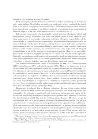
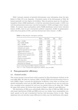
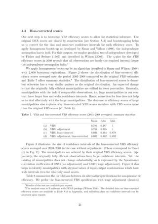
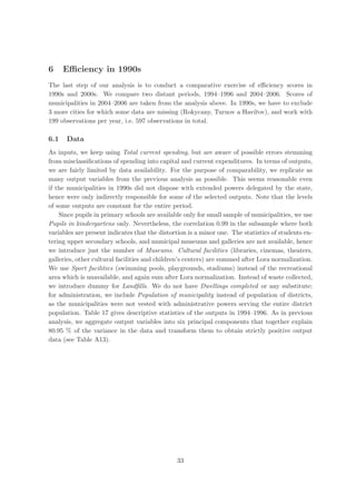
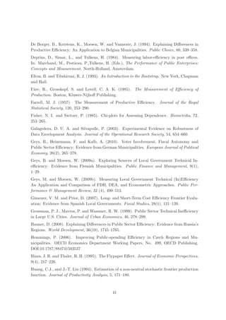
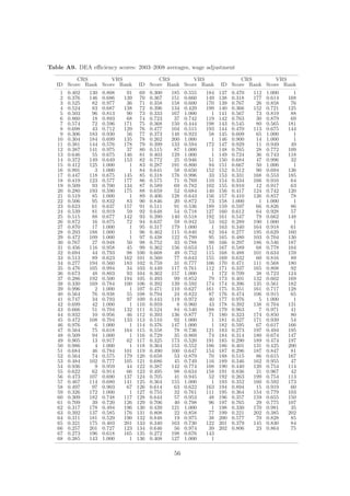
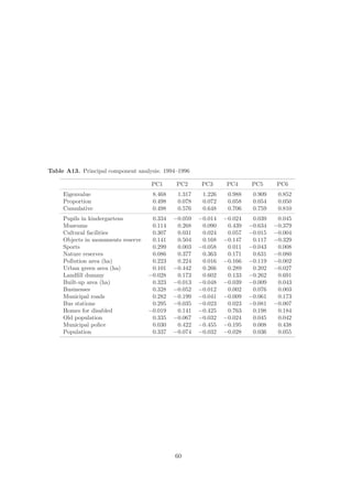
44. A Methodology
A.1 Data Envelopment Analysis
Let X denote the input matrix of dimension N × p, where p denotes the total number of
inputs, and Y denotes the output-matrix of dimension N × q, where q is the number of
outputs. Municipality i ∈ {1, . . . , N } uses inputs xi to produce outputs yi . The objective
is to find θi ∈ [0, 1], representing the maximal possible proportion by which original inputs
used by municipality i can be contracted such that given level of outputs remains feasible.
Efficiency score of municipality i, θi , is obtained by solving the following problem:
min θi s.t. −yi + Yλi ≥ 0
θi ,λi
θi xi − Xλi ≥ 0 (7)
λ≥0
Here θi is scalar and λi is vector of N constants. Inputs xi can be radially contracted to θi xi
such that yi is feasible under given technology. This radial contraction of the input vector
produces a projected point (Xλi ,Yλi ), which is a linear combination of the observed data
weighted by vector λi and lies on the surface of the technology.
This optimization problem is solved separately for each of the N municipalities, therefore
each municipality i is assigned its specific set of weights λi . The vector λi reflects which
municipalities form the efficient benchmark for the municipality i. Municipality j affects θi
if λij > 0. We call these influential observations as peers.
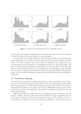
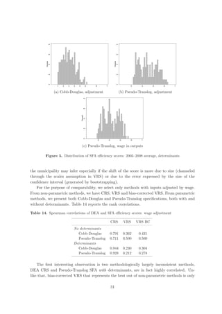
Efficiency computed from the model in (7) is based on underlying assumption of constant
returns to scale (CRS) technology, as in the original paper by Charnes et al. (1978). Banker
et al. (1984) extend the analysis to account for variable returns to scale (VRS) technology by
adding additional convexity constraint
N
λij = 1. (8)
j=1
This constraint ensures that an inefficient municipality is only benchmarked against peers
of a similar size. We can easily adjust the model to non-increasing returns to scale (NIRS)
(F¨re et al. 1985). Under this restriction, the municipality i is not benchmarked against
a
substantially larger municipalities, but may be compared with smaller municipalities. NIRS
technology is generated by substituting the restriction (8) by
N
λij ≤ 1. (9)
j=1
44

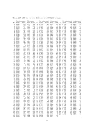
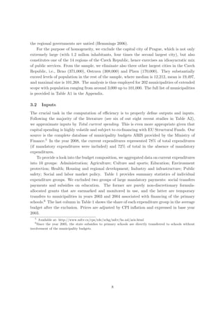
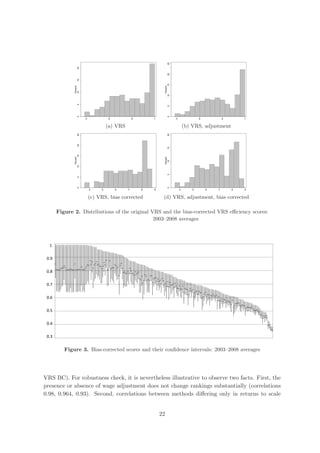
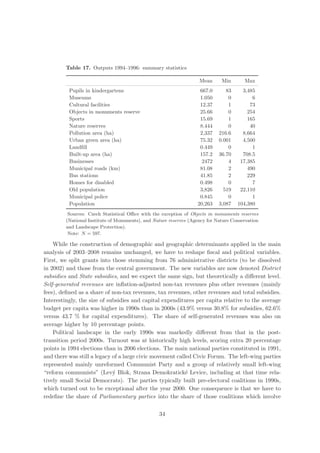
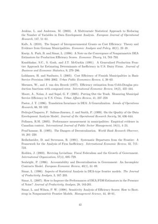
45. A.2 Outliers
Wilson (1993) provides a diagnostic statistics which may help to identify outliers, but this
approach is computationally infeasible for large data sets. Nevertheless, for our case the
statistic is computable. The statistic represents the proportion of the geometric volume in
input × output space spanned by a subset of the data obtained by deleting given number of
observations relative to the volume spanned by the entire data set. Those sets of observations
deleted from the sample that produce small values of the statistic are considered to be outliers.
As noticed in Wilson (1993), the statistics may fail to identify outliers if the effect of one outlier
is masked by one or more other outliers. Therefore, it is reasonable to combine this detection
method with alternative methods.
Cazals et al. (2002) have introduced the concept of partial frontiers (order-m frontiers)
with a nonparametric estimator which does not envelop all the data points. Order-m efficiency
score can be viewed as the expectation of the minimal input efficiency score of the unit i,
when compared to m units randomly drawn from the population of units producing at least
the output level produced by i, therefore the score is not bounded at unity. An alternative
to order-m partial frontiers are quantile based partial frontiers proposed by Aragon et al.
(2005), extended to multivariate setting by Daouia and Simar (2007). The idea is to replace
this concept of “discrete” order-m partial frontier by a “continuous” order-α partial frontier,
where α ∈ [0, 1]. Simar (2007) proposed an outlier detection strategy based on order-m
frontiers. If an observation remains outside the order-m frontier as m increases, then this
observation may be an outlier.
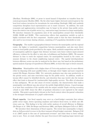
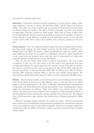
In our case, we construct order-m efficiency scores for m = 25, 50, 100, 150. The number
of super-efficient observations decreases in m. For m = 100 we have 3–6 (depending on the
year) observations with θm > 1 and 1–3 observations with θm > 1.01. To find if these outliers
influence efficiency of other observations, i.e. if they constitute peers, we compute basic DEA
efficiency scores and explore super-efficient observations serving as peers. In the next step,
we scrutinize observations having our potential outliers as peers. We compare their efficiency
scores θDEA and θm . If an observation is super-efficient (θm > 1 for relatively large m) and
if it has low θDEA score, then it may be distorted by the presence of the outliers. We find
no super-efficient observation with a low DEA score, hence our super-efficient values do not
distort efficiency rankings.
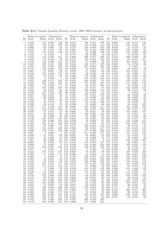
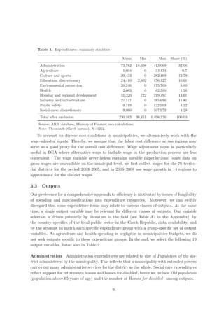
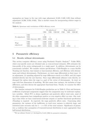
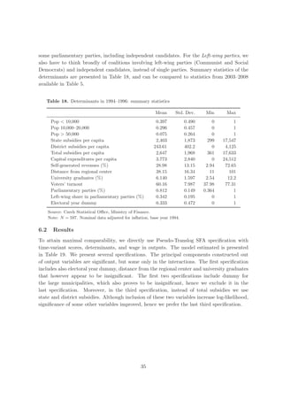
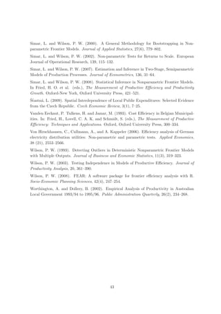
A.3 Bootstrap in DEA
DEA efficiency estimates are subject to uncertainty due to sampling variation. To allow for
statistical inference, we need to know statistical properties of the nonparametric estimators,
therefore to define a statistical model that describes the data generating process (Simar 1996),
i.e. the process yielding the data observed in the sample (X, Y).
Once we define a statistical model (see for example Kneip et al. 1998), we can apply
ˆ
bootstrap technique to provide approximations of the sampling distributions of θ(X, Y) −
ˆ
θ(X, Y), where θ(X, Y) is the DEA estimator and θ(X, Y ) is the true value of efficiency.
45

46. Knowledge of the sampling distribution allows us to evaluate the bias, the standard deviation
ˆ
of θ(X, Y), and to derive bounds of confidence intervals for θ(X, Y). Simar and Wilson (2000)
describe the methodology for bootstrapping in non-parametric models.
ˆ
The bootstrap bias estimate δ can be obtained from:
B
ˆ ˆ 1 ˆ∗ ˆ
δ(θ(X, Y)) ≈ θb (X, Y) − θ(X, Y), (10)
B
b=1
ˆ
where the bias estimate δ is the difference between mean of the Monte-Carlo realizations of
ˆ (X, Y)}B and DEA efficiency estimator. Hence, the original DEA efficiency estimator
∗
{θb b=1
may be corrected for the bias.
˜ ˆ ˆ ˆ
θ(X, Y) = θ(X, Y) − δ(θ(X, Y) (11)
ˆ ˆ
However, Efron and Tibshirani (1993), recommend not to correct for the bias unless |δ(θ(X, Y))| >
ˆ ˆ ˆ ˆ
σ (θ(X, Y))/4, where σ (θ(X, Y)) is a standard deviation, i.e. a square-root of the variance of
the bootstrap distribution:
B B
1 1 2
ˆ ˆ
2
σ (θ(X, Y)) ≈ ˆ∗
θb (X, Y) − ˆ∗
θb (X, Y) (12)
B B
b=1 b=1
The bootstrap is consistent if the available bootstrap distribution mimics the original
unknown sampling distribution. The naive bootstrap procedure, however, does not satisfy
this condition because of the boundary estimation framework (Efron and Tibshirani 1993).
Simar and Wilson (1998) propose the homogenous smooth bootstrap which can be applied to
overcome this problem. This procedure can be used only if independence assumption holds,
i.e. under independence between technical inefficiency and output levels as well as the mix of
inputs. Wilson (2003) provides a survey of tests for independence. We employ the graphical
method developed by Fisher and Switzer (1985).
46

47. B Data and results
Figure A1. Districts administered by municipalities of extended scope in the Czech Republic
47

48. Table A1. List of municipalities
1 Beneˇov s 69 Litomˇˇiceer 137 Boskovice
2 Beroun 70 Litv´ ınov 138 Bˇeclav
r
3 Brand´s nad Labem-Star´ Boleslav 71
y a Louny 139 Buˇovice
c
4 ˇa
C´slav 72 Lovosice 140 Hodon´ ın
5 ˇ
Cernoˇice s 73 Most 141 Hustopeˇe c
6 ˇ
Cesk´ Brod
y 74 Podboˇany r 142 Ivanˇice
c
7 Dobˇ´srıˇ 75 Roudnice nad Labem 143 Kuˇim
r
8 Hoˇovice
r 76 Rumburk 144 Kyjov
9 Kladno 77 Teplice 145 Mikulov
10 Kol´ ın 78 ´ ı
Ust´ nad Labem 146 Moravsk´ Krumlov
y
11 Kralupy nad Vltavou 79 Varnsdorf 147 Pohoˇelice
r
12 Kutn´ Hora
a 80 ˇ
Zatec 148 Rosice
13 Lys´ nad Labem
a 81 ˇ
Cesk´ L´a ıpa 149 Slavkov u Brna
14 Mˇln´
e ık 82 Fr´dlant
y 150 ˇ
Slapanice
15 Mlad´ Boleslav
a 83 Jablonec nad Nisou 151 Tiˇnov
s
16 Mnichovo Hradiˇtˇ s e 84 Jilemnice 152 Vesel´ nad Moravou
ı
17 Neratovice 85 Liberec 153 Vyˇkov
s
18 Nymburk 86 Nov´ Bor
y 154 Znojmo
19 Podˇbrady
e 87 Semily 155 ˇ
Zidlochovice
20 Pˇ´
rıbram 88 Tanvald 156 Hranice
21 Rakovn´ ık 89 Turnov 157 Jesen´ ık
22 ˇ ıˇ
R´cany 90 ˇ
Zelezn´ Brod
y 158 Konice
23 Sedlˇany
c 91 Broumov 159 Lipn´ nad Beˇvou
ık c
24 Slan´ y 92 Dobruˇka s 160 Litovel
25 Vlaˇim
s 93 Dv˚ Kr´lov´ nad Labem
ur a e 161 Mohelnice
26 Votice 94 Hoˇice
r 162 Olomouc
27 Blatn´ a 95 Hradec Kr´lov´ a e 163 Prostˇjove
28 ˇ
Cesk´ Budˇjovice
e e 96 Jaromˇˇ er 164 Pˇerov
r
29 ˇ
Cesk´ Krumlov
y 97 Jiˇ´
cın 165 ˇ
Sternberk
30 Daˇice
c 98 Kostelec nad Orlic´ ı 166 ˇ
Sumperk
31 Jindˇich˚ Hradec
r uv 99 N´chod
a 167 Uniˇov
c
32 Kaplice 100 Nov´ Paka
a 168 Z´bˇeh
a r
33 Milevsko 101 Nov´ Mˇsto nad Metuj´
e e ı 169 Bystˇice pod Host´nem
r y
34 P´ısek 102 Nov´ Bydˇov
y z 170 Holeˇovs
35 Prachatice 103 Rychnov nad Knˇznou e 171 Kromˇˇ´z erıˇ
36 Sobˇslav
e 104 Trutnov 172 Luhaˇovice
c
37 Strakonice 105 Vrchlab´ ı 173 Otrokovice
38 T´bor
a 106 ˇ
Cesk´ Tˇebov´
a r a 174 Roˇnov pod Radhoˇtˇm
z s e
39 Trhov´ Sviny
e 107 Hlinsko 175 Uhersk´ Hradiˇtˇ
e s e
40 Tˇeboˇ
r n 108 Holice 176 Uhersk´ Brody
41 T´n nad Vltavou
y 109 Chrudim 177 Valaˇsk´ Klobouky
s e
42 Vimperk 110 Kr´l´
a ıky 178 Valaˇsk´ Meziˇ´c´
s e rıˇı
43 Vodˇany
n 111 Lanˇkroun
s 179 Vizovice
44 Blovice 112 Litomyˇl s 180 Vset´ ın
45 Domaˇlice z 113 Moravsk´ Tˇebov´
a r a 181 Zl´ın
46 zˇ
Horaˇdovice 114 Pardubice 182 B´ılovec
47 Horˇovsk´ T´n
s y y 115 Poliˇka
c 183 Bohum´ ın
48 Klatovy 116 Pˇelouˇ
r c 184 Brunt´l a
49 Kralovice 117 Svitavy 185 ˇ
Cesk´ Tˇˇ´
y esın
50 Nepomuk 1185 ´ ı
Ust´ nad Orlic´ ı 186 Frenˇt´t pod Radhoˇtˇm
s a s e
51 N´ˇany
yr 119 Vysok´ M´to
e y 187 Fr´dek-M´
y ıstek
52 Pˇeˇtice
r s 120 ˇ
Zamberk 188 Fr´dlant nad Ostravic´
y ı
53 Rokycany 121 Bystˇice nad Pernˇtejnem
r s 189 Hav´rov
ıˇ
54 Stod 122 Havl´ck˚ Brod
ıˇ uv 190 Hluˇ´cın
55 Stˇ´
rıbro 123 Humpolec 191 Jablunkov
56 Suˇice
s 124 Chotˇboˇ e r 192 Karvin´ a
57 Tachov 125 Jihlava 193 Kopˇivnice
r
58 Aˇs 126 Moravsk´ Budˇjovice
e e 194 Kravaˇe r
59 Cheb 127 N´mˇˇˇ nad Oslavou
a est 195 Krnov
60 Karlovy Vary 128 Nov´ Mˇsto na Moravˇ
e e e 196 Nov´ Jiˇ´
y cın
61 Kraslice 129 Pacov 197 Odry
62 Mari´nsk´ L´znˇ
a e a e 130 Pelhˇimov
r 198 Opava
63 Ostrov 131 Svˇtl´ nad S´zavou
e a a 199 Orlov´ a
64 Sokolov 132 Telˇ c 200 R´maˇov
y r
65 B´ılina 133 Tˇeb´c
r ıˇ 201 Tˇinec
r
66 Dˇˇ´
ecın 134 Velk´ Meziˇ´c´
e rıˇı 202 V´ıtkov
67 Chomutov 135 ˇ ˇa
Zd´r nad S´zavou a
68 Kadaˇ n 136 Blansko48

49. Table A2. Selected studies on comprehensive efficiency of local governments
Authors Country N Period Method(s) Inputs Outputs
Afonso and Fer- Portugal 278 2001 DEA Total expenditures Old people, no. of schools, school enrolment, share
nandes (2008) per capita of library users in population, water supply, solid
waste, licenses for building construction, length of
roads per population
Arcelus et al. Spain: 263 1998–2001 SFA BC Total current Area, total population, share of old people,
(2007) Navarre region expenditures dwellings, index measuring the scarcity in the pro-
vision of municipal services, time trend
Balaguer-Coll et Spain: 414 1995 DEA, FDH Wages and salaries, Population, no. of lighting points, tons of waste,
al. (2007) Valencian region expenditure on goods street infrastructure area, public parks area, qual-
and services, cur- ity services (good, average, bad)
rent transfers, capital
transfers, capital ex-
penditures
De Borger and Belgium 589 1985 DEA, FDH, Total current No. of beneficiaries of minimal subsistence grants,
Kerstens (1996) SFA, COLS expenditures students in local primary schools, surface of pub-
lic recreational facilities, population, share of old
49
people
Geys et al. (2010) Germany: 1021 2001 SFA BC Total current Students in local public schools, kindergartens,
Baden- expenditures surface of public recreational facilities, popula-
Wurtenberg tion, old people, no. of employees paying social
security contributions
Geys and Moesen Belgium: 300 2000 SFA BC Current expendi- Number of subsistence grant beneficiaries, number
(2009) Flanders tures on those issues of students in local primary schools, size of public
for which we observe recreational facilities, length of municipal roads,
government outputs share of municipal waste collected through door-
to-door collections
Kalb (2010) Germany: 245 1990–2004 SFA BC Total current Students in public schools, population, share of
Baden- expenditures old people, number of employees covered by social
Wurtenberg security, surface of public recovery areas
Vanden Eeckaut Belgium: 235 1986 DEA, FDH Total current Population, length of roads, old people, no. of
et al. (1993) Wallone region expenditures beneficiaries of minimal subsistence grants, no. of
crimes
Note: We denote the method developed by Battese and Coelli (1995) as SFA BC, and corrected ordinary
least squares as COLS.

50. Table A3. Output variables
Source Database Web page Available Note
Pupils in primary schools IIE Aggregated data http://stistko.uiv.cz/vo/ 2003–2008
and kindergartens
Pupils entering secondary IIE Aggregated data http://stistko.uiv.cz/vo/ 2005–2008 2005–2008 average for 2003–2004
schools (%)
Cultural facilities CZSO City and municipal 2003–2006 2006 data for 2007–2008
statistics (MOS)
Municipal museums and MGA, munici- Catalog of museums http://www.cz-museums.cz/ Retrieved in 2009 Same for 2003–2008
galleries pal websites and galleries amg/faces/adresar/
Objects in monuments re- NIM Monumnet http://monumnet.npu.cz/ 2003–2008 Objects in municipal monuments
serve monumnet.php reserves and zones
Sporting and recreational CZSO MOS 2006–2008 2006 data for 2003–2005
area (ha)
Municipal waste (tons) ME ISOH http://isoh.cenia.cz/groupisoh 2003–2008 Data for ORP districts adjusted for
population share of a municipality
in whole district population
Nature reserves ANCLP USOP http://drusop.nature.cz/ 2003–2008 Sum of national nature reserves, na-
50
ture reserves, national nature mon-
uments and nature monuments
Pollute area (ha) CZSO MOS 2003–2008 Sum of arable land, built-up and
other area
Urban green area (ha) CZSO MOS 2006–2008 2006 data for 2003–2005
Built-up area (ha) CZSO MOS 2003–2008
New dwellings CZSO MOS 2003–2008
Businesses CZSO MOS 2003–2008
Municipal roads (ha) CZSO MOS 2006–2008 2006 data for 2003–2005
Bus stations IDOS http://jizdnirady.idnes.cz/ Retrieved in 2009 Same for 2003–2008
Population in district CZSO Regional Yearbooks http://www.czso.cz/csu/ 2003–2008
redakce.nsf/i/krajske rocenky
Old population CZSO MOS 2003–2008
Homes for disabled CZSO MOS 2003–2006 2006 data for 2007–2008
Municipal police MOS, municipal 2003–2008
websites
Sources: ANCLP = Agency for Nature Conservation and Landscape Protection, MGA = Museums and Gal-
leries Association, CZSO = Czech Statistical Office, IDOS = Transportation timetables, IIE = Institute for
Information on Education, ME = Ministry of Environment, NIM= National Institute of Monuments.

51. Table A4. Correlation matrix of output variables
A B C D E F G H I J K L M N O P Q RS
Pupils in prim. schools and kindergart. A 1
Pupils entering secondary schools (%) B −0.150 1
Cultural facilities C 0.820 −0.080 1
Municipal museums and galleries D −0.220 0.082 −0.063 1
Objects in monuments reserve E 0.305 0.070 0.353 −0.028 1
Sporting and recreational area (ha) F 0.554 −0.066 0.472 −0.099 0.362 1
Municipal waste (tons) G 0.839 −0.110 0.642 −0.179 0.228 0.459 1
Nature reserves H 0.180 −0.026 0.146 −0.208 0.278 0.176 0.104 1
Pollute area (ha) I 0.588 −0.086 0.644 −0.001 0.419 0.537 0.456 0.117 1
51
Urban green area (ha) J 0.819 −0.146 0.657 −0.218 0.155 0.518 0.651 0.088 0.480 1
Built-up area (ha) K 0.922 −0.122 0.829 −0.185 0.388 0.579 0.797 0.178 0.672 0.702 1
New dwellings L 0.587 −0.006 0.545 −0.166 0.398 0.395 0.555 0.204 0.414 0.435 0.664 1
Businesses M 0.949 −0.104 0.817 −0.221 0.351 0.577 0.835 0.214 0.560 0.764 0.934 0.685 1
Municipal roads (ha) N 0.706 −0.090 0.681 −0.068 0.351 0.600 0.578 0.140 0.801 0.637 0.710 0.451 0.702 1
Bus stations O 0.767 −0.067 0.615 −0.096 0.221 0.325 0.677 0.175 0.408 0.573 0.700 0.432 0.730 0.524 1
Population in district P 0.884 −0.151 0.721 −0.274 0.338 0.511 0.791 0.355 0.503 0.689 0.855 0.619 0.886 0.582 0.692 1
Old population Q 0.968 −0.124 0.852 −0.226 0.339 0.571 0.840 0.175 0.585 0.803 0.945 0.667 0.971 0.702 0.725 0.888 1
Homes for disabled R 0.559 −0.075 0.413 −0.180 0.110 0.199 0.482 0.123 0.299 0.455 0.533 0.235 0.512 0.406 0.443 0.496 0.511 1
Municipal police S 0.230 0.074 0.166 −0.017 0.135 0.175 0.187 0.131 0.053 0.200 0.220 0.094 0.222 0.121 0.176 0.270 0.217 0.162 1
Note: N=1212.

52. Table A5. Determinants and price level normalizations
Source Database Web page Available Note
Population CZSO Regional http://www.czso.cz/csu/ 2003–2008
Yearbooks redakce.nsf/i/krajske rocenky
University graduates CZSO Census 2001 2001 for 2003–2008
Subsidies MF ARIS http://wwwinfo.mfcr.cz/aris/ 2003–2008 Total state subsidies
Self-generated revenues MF ARIS http://wwwinfo.mfcr.cz/aris/ 2003–2008 Charges and fees, real estate tax and non-tax
revenues / Total revenues (own transfers ex-
cluded)
Lagged debt dummy MF ARIS http://wwwinfo.mfcr.cz/aris/ 2003–2008 Deficit after consolidation
Distance Map server Mapy.cz http://www.mapy.cz 2010 The shortest distance in minutes
Political concentration CZSO Election http://volby.cz/ 2002, 2006 2002 results for 2003–2006, 2006 results for
server 2007–2008, Hirschmann-Herfindahl index
52
Left-wing parties CZSO Election http://volby.cz/ 2002, 2006 2002 results for 2003–2006, 2006 results for
server ˇ
2007–2008, the share of seats of KSCM and
ˇ
CSSD
Parliamentary parties CZSO Election http://volby.cz/ 2002, 2006 2002 results for 2003–2006, 2006 results for
server ˇ
2007–2008, the share of seats of CSSD, KDU-
ˇ ˇ
CSL, KSCM, ODS, US-DEU
Turnout CZSO Election http://volby.cz/ 2002, 2006 2002 elections for 2003–2006, 2006 elections for
server 2007–2008
Wage CZSO KROK 2003–2005 2005 data for districts (okresy), 2006–2008
data based on 2005 but adjusted for growths
of regional gross wages (13 regions)
Inflation CZSO http://www.czso.cz/ 2003–2008 CPI, 2003 base year
Sources: CZSO = Czech Statistical Office, MF = Ministry of Finance of the Czech Republic.

53. Table A6. Correlation matrix of determinants
A B C D E F G H I J K L MN
Pop < 10,000 A 1
Pop 10,000–20,000 B −0.551 1
Pop > 50,000 C −0.249 −0.208 1
University graduates (%) D −0.378 −0.020 0.385 1
Subsidies per capita E 0.208 −0.045 −0.162 −0.114 1
Capital expenditures per capita F 0.059 −0.024 −0.051 0.019 0.383 1
53
Lagged debt dummy G 0.014 0.027 −0.021 −0.046 −0.044 −0.094 1
Self-generated revenues (%) H −0.044 0.028 −0.088 0.026 −0.110 −0.076 0.048 1
Distance from regional center I −0.075 0.080 0.071 −0.033 −0.001 0.070 0.008 −0.052 1
Voters’ turnout J 0.616 −0.088 −0.395 −0.104 0.267 0.147 −0.028 0.051 −0.043 1
Political concentration K −0.060 −0.086 0.233 0.047 0.004 −0.039 −0.022 0.177 −0.108 −0.116 1
Left-wing share L −0.212 −0.001 0.148 −0.110 −0.169 −0.054 0.015 0.039 0.011 −0.450 0.073 1
Parliamentary parties share M −0.331 0.050 0.197 0.079 −0.171 −0.013 0.015 0.063 −0.011 −0.314 0.234 0.075 1
Electoral year N −0.002 0.002 −0.003 0.000 −0.214 0.097 0.077 0.107 0.000 −0.006 −0.047 0.032 0.035 1
Note: N=1212.

54. Table A7. Year-specific DEA efficiency scores
No adjustment Wage adjustment
Mean Min # Fully eff. Mean Min # Fully eff.
2003 CRS 0.545 0.213 9 0.540 0.207 9
NIRS 0.780 0.320 60 0.785 0.333 55
VRS 0.781 0.320 60 0.787 0.333 55
2004 CRS 0.442 0.145 4 0.457 0.151 4
NIRS 0.782 0.279 56 0.787 0.284 56
VRS 0.782 0.279 56 0.788 0.284 56
2005 CRS 0.548 0.239 9 0.552 0.246 7
NIRS 0.788 0.342 52 0.787 0.351 48
VRS 0.788 0.342 52 0.788 0.351 48
2006 CRS 0.540 0.247 5 0.550 0.246 8
NIRS 0.776 0.383 52 0.771 0.371 53
VRS 0.776 0.383 53 0.772 0.371 54
2007 CRS 0.519 0.226 6 0.536 0.227 7
NIRS 0.798 0.376 61 0.781 0.365 53
VRS 0.798 0.376 61 0.782 0.365 53
2008 CRS 0.519 0.226 6 0.530 0.235 10
NIRS 0.788 0.380 52 0.786 0.395 52
VRS 0.788 0.380 52 0.786 0.395 52
Average CRS 0.519 0.145 1 0.528 0.151 1
NIRS 0.785 0.279 30 0.783 0.284 31
VRS 0.786 0.279 30 0.784 0.284 31
54

55. Table A8. DEA efficiency scores: 2003–2008 averages, no adjustment
CRS VRS CRS VRS CRS VRS
ID Score Rank Score Rank ID Score Rank Score Rank ID Score Rank Score Rank
1 0.395 133 0.786 104 69 0.299 180 0.551 185 137 0.477 104 1.000 1
2 0.311 176 0.573 179 70 0.320 171 0.568 181 138 0.327 168 0.630 159
3 0.435 120 0.849 84 71 0.368 145 0.617 165 139 0.771 26 0.875 75
4 0.473 107 0.635 157 72 0.384 139 0.430 199 140 0.379 141 0.746 115
5 0.400 130 0.693 137 73 0.289 183 1.000 1 141 0.593 68 0.824 91
6 0.798 22 0.826 89 74 0.772 25 0.788 103 142 0.708 36 0.812 93
7 0.582 71 0.611 168 75 0.361 147 0.435 198 143 0.521 88 0.539 189
8 0.579 72 0.592 174 76 0.462 111 0.505 192 144 0.489 98 0.698 135
9 0.271 194 0.918 64 77 0.348 154 0.940 56 145 0.613 63 1.000 1
10 0.283 188 0.648 154 78 0.230 201 1.000 1 146 0.962 4 1.000 1
11 0.333 164 0.497 195 79 0.403 129 0.614 167 147 0.924 8 0.956 45
12 0.336 161 0.948 50 80 0.533 85 1.000 1 148 0.720 32 0.736 119
13 0.625 61 0.664 149 81 0.368 144 1.000 1 149 0.717 33 0.759 111
14 0.322 170 0.564 182 82 0.709 35 0.904 66 150 0.626 60 0.987 37
15 0.314 172 0.951 49 83 0.284 187 0.876 74 151 0.616 62 0.985 38
16 0.798 23 1.000 1 84 0.652 52 0.680 142 152 0.525 86 0.707 130
17 0.394 134 0.620 163 85 0.285 186 0.989 36 153 0.349 153 0.578 176
18 0.429 121 0.598 171 86 0.515 91 0.690 138 154 0.360 149 0.995 34
19 0.538 83 0.698 134 87 0.603 66 0.790 102 155 0.847 18 0.881 71
20 0.277 192 0.631 158 88 0.650 53 0.698 133 156 0.404 128 0.748 114
21 0.488 99 1.000 14 89 0.407 126 0.662 150 157 0.449 116 0.933 58
22 0.423 122 0.716 125 90 0.866 15 0.863 77 158 1.000 1 1.000 1
23 0.628 59 0.643 155 91 0.556 78 0.576 177 159 0.588 69 0.854 81
24 0.469 108 0.801 98 92 0.663 48 0.743 116 160 0.571 73 0.898 68
25 0.515 90 0.667 147 93 0.398 131 0.519 191 161 0.560 76 0.669 145
26 0.870 14 0.882 70 94 0.649 55 0.930 60 162 0.279 191 1.000 1
27 0.852 16 1.000 1 95 0.283 189 1.000 1 163 0.343 156 0.984 39
28 0.253 199 1.000 1 96 0.485 101 0.889 69 164 0.275 193 0.676 143
29 0.462 112 1.000 1 97 0.446 117 0.806 97 165 0.464 109 0.716 126
30 0.849 17 0.990 35 98 0.758 27 0.811 94 166 0.305 178 0.558 184
31 0.490 96 0.996 33 99 0.383 140 0.709 128 167 0.559 77 0.758 112
32 0.678 43 0.768 110 100 0.676 45 0.778 108 168 0.499 94 0.665 148
33 0.545 81 0.660 151 101 0.609 65 0.715 127 169 0.647 57 0.839 86
34 0.294 181 0.621 162 102 0.690 38 0.701 131 170 0.490 97 0.595 172
35 0.496 95 1.000 1 103 0.443 119 0.756 113 171 0.340 157 0.866 76
36 0.666 47 0.808 95 104 0.362 146 1.000 1 172 0.655 50 0.685 139
37 0.285 185 0.495 196 105 0.506 92 0.858 79 173 0.376 143 0.564 183
38 0.330 166 0.839 85 106 0.411 124 0.618 164 174 0.389 135 0.544 188
39 0.901 12 0.967 40 107 0.482 103 0.651 153 175 0.356 150 0.722 122
40 0.585 70 0.967 41 108 0.716 34 0.741 118 176 0.486 100 0.938 57
41 0.687 41 0.779 107 109 0.455 114 1.000 1 177 0.921 10 1.000 1
42 0.728 31 1.000 1 110 0.960 5 0.960 44 178 0.386 136 0.684 140
43 0.674 46 0.742 117 111 0.546 80 0.589 175 179 0.895 13 0.952 48
44 0.926 7 0.941 55 112 0.405 127 0.908 65 180 0.305 177 0.853 82
45 0.463 110 0.682 141 113 0.534 84 1.000 1 181 0.313 173 0.941 54
46 0.998 2 1.000 1 114 0.338 160 1.000 1 182 0.550 79 0.574 178
47 0.560 75 0.616 166 115 0.601 67 0.800 99 183 0.271 195 0.530 190
48 0.524 87 1.000 1 116 0.653 51 0.799 100 184 0.335 162 0.719 124
49 0.913 11 0.926 62 117 0.338 159 0.550 187 185 0.289 184 0.478 197
50 0.980 3 1.000 1 118 0.385 137 0.592 173 186 0.385 138 0.407 200
51 0.689 39 0.806 96 119 0.503 93 0.668 146 187 0.282 190 0.850 83
52 0.567 74 0.570 180 120 0.686 42 0.903 67 188 0.475 105 0.609 169
53 0.445 118 0.732 121 121 0.688 40 0.732 120 189 0.346 155 0.997 31
54 0.924 9 0.948 51 122 0.396 132 0.826 90 190 0.460 113 0.777 109
55 0.647 56 0.943 52 123 0.516 89 0.636 156 191 0.819 20 0.967 42
56 0.484 102 0.697 136 124 0.737 29 0.955 46 192 0.262 197 0.829 88
57 0.474 106 0.671 144 125 0.311 175 0.996 32 193 0.326 169 0.551 186
58 0.540 82 0.965 43 126 0.655 49 0.657 152 194 0.944 6 0.931 59
59 0.338 158 1.000 1 127 0.782 24 0.798 101 195 0.378 142 0.835 87
60 0.313 174 0.816 92 128 0.650 54 0.943 53 196 0.330 165 0.607 170
61 0.676 44 0.700 132 129 0.749 28 0.878 73 197 0.707 37 0.720 123
62 0.327 167 0.500 193 130 0.455 115 1.000 1 198 0.334 163 1.000 1
63 0.408 125 0.627 160 131 0.817 21 0.928 61 199 0.216 202 0.387 202
64 0.293 182 0.500 194 132 0.733 30 0.925 63 200 0.612 64 0.855 80
65 0.303 179 0.394 201 133 0.353 152 0.785 105 201 0.355 151 0.859 78
66 0.251 200 0.781 106 134 0.645 58 0.954 47 202 0.819 19 0.880 72
67 0.259 198 0.625 161 135 0.268 196 0.707 129
68 0.361 148 1.000 1 136 0.420 123 1.000 1
55

56. Table A9. DEA efficiency scores: 2003–2008 averages, wage adjustment
CRS VRS CRS VRS CRS VRS
ID Score Rank Score Rank ID Score Rank Score Rank ID Score Rank Score Rank
1 0.402 130 0.808 91 69 0.300 185 0.555 184 137 0.470 112 1.000 1
2 0.376 146 0.686 139 70 0.367 151 0.660 149 138 0.318 177 0.614 168
3 0.525 82 0.977 36 71 0.358 158 0.600 170 139 0.767 26 0.858 76
4 0.524 83 0.687 138 72 0.396 134 0.429 199 140 0.366 152 0.721 125
5 0.503 96 0.813 90 73 0.333 167 1.000 1 141 0.567 73 0.819 88
6 0.860 18 0.893 68 74 0.723 37 0.742 119 142 0.763 30 0.879 69
7 0.574 72 0.596 171 75 0.368 150 0.444 198 143 0.545 80 0.565 181
8 0.698 43 0.712 129 76 0.477 104 0.515 193 144 0.470 113 0.675 144
9 0.306 183 0.930 56 77 0.373 148 0.923 58 145 0.609 65 1.000 1
10 0.304 184 0.699 135 78 0.262 200 1.000 1 146 0.900 14 1.000 1
11 0.381 144 0.576 178 79 0.399 133 0.594 172 147 0.929 11 0.949 49
12 0.387 141 0.975 37 80 0.515 87 1.000 1 148 0.765 28 0.772 109
13 0.646 55 0.675 146 81 0.403 129 1.000 1 149 0.724 36 0.743 118
14 0.372 149 0.649 153 82 0.772 25 0.946 51 150 0.684 47 0.996 32
15 0.412 125 1.000 1 83 0.287 191 0.800 94 151 0.667 50 1.000 1
16 0.991 3 1.000 1 84 0.641 58 0.650 152 152 0.512 90 0.694 136
17 0.447 118 0.675 145 85 0.318 176 0.996 33 153 0.331 168 0.553 185
18 0.419 123 0.577 177 86 0.575 71 0.769 110 154 0.334 166 0.916 64
19 0.509 93 0.700 134 87 0.589 69 0.782 102 155 0.910 12 0.917 63
20 0.280 193 0.590 175 88 0.659 52 0.684 140 156 0.417 124 0.742 120
21 0.519 85 1.000 1 89 0.406 128 0.643 156 157 0.410 126 0.857 78
22 0.506 95 0.832 83 90 0.846 20 0.872 73 158 1.000 1 1.000 1
23 0.623 61 0.637 157 91 0.511 91 0.536 189 159 0.597 66 0.826 86
24 0.539 81 0.919 59 92 0.648 54 0.718 127 160 0.612 64 0.928 57
25 0.515 88 0.677 142 93 0.390 140 0.518 192 161 0.547 79 0.662 148
26 0.872 16 0.875 72 94 0.637 59 0.942 53 162 0.289 190 1.000 1
27 0.870 17 1.000 1 95 0.317 179 1.000 1 163 0.340 164 0.918 61
28 0.293 188 1.000 1 96 0.462 115 0.840 82 164 0.277 195 0.629 160
29 0.472 109 1.000 1 97 0.438 122 0.799 95 165 0.480 103 0.704 130
30 0.767 27 0.948 50 98 0.752 33 0.788 99 166 0.297 186 0.546 187
31 0.456 116 0.958 45 99 0.362 156 0.653 151 167 0.589 68 0.778 104
32 0.694 44 0.793 98 100 0.668 49 0.752 115 168 0.488 101 0.634 159
33 0.513 89 0.623 162 101 0.560 77 0.643 155 169 0.632 60 0.816 89
34 0.277 194 0.560 183 102 0.759 31 0.777 106 170 0.471 111 0.568 180
35 0.476 105 0.994 34 103 0.449 117 0.761 112 171 0.337 165 0.808 92
36 0.673 48 0.803 93 104 0.362 157 1.000 1 172 0.709 38 0.723 124
37 0.286 192 0.500 194 105 0.493 99 0.852 79 173 0.401 132 0.602 169
38 0.330 169 0.784 100 106 0.392 139 0.592 174 174 0.396 135 0.561 182
39 0.996 2 1.000 1 107 0.471 110 0.627 161 175 0.351 161 0.717 128
40 0.564 76 0.938 55 108 0.794 24 0.822 87 176 0.474 106 0.915 65
41 0.747 34 0.793 97 109 0.443 119 0.972 40 177 0.976 5 1.000 1
42 0.699 42 1.000 1 110 0.959 8 0.960 43 178 0.392 138 0.704 131
43 0.666 51 0.704 132 111 0.524 84 0.540 188 179 0.963 7 0.971 41
44 0.932 10 0.956 46 112 0.393 136 0.877 71 180 0.323 174 0.850 80
45 0.472 108 0.704 133 113 0.510 92 1.000 1 181 0.327 171 0.939 54
46 0.976 6 1.000 1 114 0.376 147 1.000 1 182 0.595 67 0.617 166
47 0.564 75 0.618 164 115 0.558 78 0.736 121 183 0.273 197 0.494 195
48 0.509 94 1.000 1 116 0.729 35 0.869 74 184 0.314 180 0.674 147
49 0.905 13 0.917 62 117 0.325 173 0.520 191 185 0.290 189 0.474 197
50 0.986 4 1.000 1 118 0.364 153 0.552 186 186 0.401 131 0.425 200
51 0.684 46 0.784 101 119 0.490 100 0.647 154 187 0.296 187 0.847 81
52 0.564 74 0.575 179 120 0.658 53 0.879 70 188 0.515 86 0.615 167
53 0.484 102 0.777 105 121 0.686 45 0.749 116 189 0.346 162 0.955 47
54 0.936 9 0.959 44 122 0.387 142 0.774 108 190 0.440 120 0.754 114
55 0.622 62 0.914 66 123 0.495 98 0.634 158 191 0.836 21 0.967 42
56 0.473 107 0.690 137 124 0.705 41 0.945 52 192 0.263 199 0.754 113
57 0.467 114 0.680 141 125 0.364 155 1.000 1 193 0.352 160 0.592 173
58 0.497 97 0.903 67 126 0.614 63 0.622 163 194 0.894 15 0.919 60
59 0.326 172 1.000 1 127 0.755 32 0.761 111 195 0.364 154 0.779 103
60 0.309 182 0.748 117 128 0.644 57 0.953 48 196 0.357 159 0.655 150
61 0.709 39 0.720 126 129 0.706 40 0.798 96 197 0.765 29 0.775 107
62 0.317 178 0.494 196 130 0.439 121 1.000 1 198 0.330 170 0.981 35
63 0.392 137 0.585 176 131 0.808 22 0.858 77 199 0.221 202 0.385 202
64 0.311 181 0.529 190 132 0.848 19 0.975 38 200 0.577 70 0.828 85
65 0.321 175 0.403 201 133 0.340 163 0.730 122 201 0.379 145 0.830 84
66 0.257 201 0.727 123 134 0.646 56 0.974 39 202 0.806 23 0.864 75
67 0.273 196 0.618 165 135 0.272 198 0.676 143
68 0.385 143 1.000 1 136 0.408 127 1.000 1
56

57. Table A10. VRS bias-corrected efficiency scores: 2003–2008 averages
No adjustment Adjustment No adjustment Adjustment No adjustment Adjustment
ID Score Rank Score Rank ID Score Rank Score Rank ID Score Rank Score Rank
1 0.688 113 0.711 99 69 0.513 185 0.516 185 137 0.811 46 0.807 63
2 0.532 177 0.637 132 70 0.530 180 0.619 143 138 0.571 163 0.556 168
3 0.773 77 0.880 3 71 0.582 156 0.566 164 139 0.794 65 0.781 71
4 0.589 153 0.632 137 72 0.400 198 0.398 199 140 0.669 118 0.654 128
5 0.599 151 0.700 106 73 0.809 57 0.809 56 141 0.715 101 0.709 103
6 0.764 81 0.829 25 74 0.711 103 0.673 116 142 0.750 85 0.814 43
7 0.557 168 0.542 172 75 0.397 199 0.408 198 143 0.499 189 0.521 183
8 0.549 170 0.665 122 76 0.472 192 0.483 191 144 0.643 130 0.625 141
9 0.789 69 0.797 67 77 0.849 13 0.836 20 145 0.830 27 0.837 18
10 0.579 157 0.631 138 78 0.808 60 0.808 60 146 0.809 54 0.809 54
11 0.456 195 0.528 178 79 0.544 172 0.522 182 147 0.837 24 0.834 22
12 0.811 45 0.828 29 80 0.816 41 0.819 37 148 0.688 112 0.720 90
13 0.611 147 0.624 142 81 0.809 53 0.807 64 149 0.680 115 0.666 121
14 0.525 182 0.604 150 82 0.783 71 0.810 48 150 0.845 16 0.839 15
15 0.806 63 0.831 23 83 0.770 78 0.696 108 151 0.855 8 0.853 8
16 0.853 9 0.818 42 84 0.626 138 0.594 152 152 0.637 134 0.629 139
17 0.567 164 0.611 148 85 0.822 33 0.828 26 153 0.543 173 0.523 180
18 0.562 166 0.539 175 86 0.609 148 0.678 113 154 0.851 11 0.791 68
19 0.649 128 0.651 130 87 0.697 107 0.688 111 155 0.801 64 0.826 32
20 0.585 154 0.547 169 88 0.628 136 0.612 146 156 0.674 116 0.668 120
21 0.810 49 0.810 49 89 0.620 141 0.601 151 157 0.821 35 0.764 78
22 0.652 127 0.746 80 90 0.784 70 0.789 69 158 0.812 44 0.811 46
23 0.593 152 0.587 154 91 0.519 184 0.483 190 159 0.762 83 0.730 85
24 0.732 92 0.841 14 92 0.690 110 0.664 123 160 0.794 66 0.813 45
25 0.627 137 0.634 135 93 0.478 191 0.479 193 161 0.619 142 0.615 144
26 0.820 37 0.809 51 94 0.766 79 0.776 72 162 0.810 50 0.810 50
27 0.809 58 0.809 57 95 0.807 62 0.809 55 163 0.869 4 0.818 38
28 0.809 56 0.809 52 96 0.782 73 0.739 81 164 0.623 140 0.578 160
29 0.808 61 0.811 47 97 0.724 98 0.720 92 165 0.669 119 0.651 129
30 0.869 5 0.845 11 98 0.751 84 0.725 89 166 0.522 183 0.510 186
31 0.878 2 0.866 4 99 0.661 124 0.612 147 167 0.710 104 0.726 88
32 0.704 106 0.728 87 100 0.694 109 0.669 118 168 0.616 143 0.584 156
33 0.579 158 0.545 171 101 0.653 125 0.582 158 169 0.730 93 0.710 101
34 0.576 160 0.522 181 102 0.646 129 0.719 93 170 0.544 171 0.518 184
35 0.819 39 0.818 40 103 0.689 111 0.692 109 171 0.776 76 0.732 84
36 0.724 97 0.718 96 104 0.810 51 0.807 65 172 0.629 135 0.661 126
37 0.467 194 0.471 194 105 0.743 87 0.739 82 173 0.533 176 0.569 163
38 0.763 82 0.709 104 106 0.553 169 0.529 177 174 0.512 186 0.529 176
39 0.845 17 0.848 10 107 0.578 159 0.558 167 175 0.666 121 0.670 117
40 0.851 12 0.837 19 108 0.665 122 0.736 83 176 0.840 20 0.821 35
41 0.716 100 0.715 98 109 0.853 10 0.837 17 177 0.824 31 0.818 41
42 0.820 36 0.827 30 110 0.818 40 0.820 36 178 0.641 131 0.663 124
43 0.667 120 0.627 140 111 0.543 174 0.491 189 179 0.879 1 0.884 2
44 0.823 32 0.843 13 112 0.793 68 0.767 77 180 0.711 102 0.709 102
45 0.613 145 0.636 134 113 0.809 52 0.809 58 181 0.827 28 0.828 28
46 0.826 29 0.827 31 114 0.809 59 0.807 62 182 0.531 178 0.573 162
47 0.528 181 0.527 179 115 0.706 105 0.642 131 183 0.494 190 0.459 195
48 0.838 21 0.850 9 116 0.745 86 0.805 66 184 0.625 139 0.585 155
49 0.857 7 0.855 7 117 0.509 187 0.479 192 185 0.450 196 0.447 196
50 0.825 30 0.822 34 118 0.539 175 0.499 187 186 0.379 200 0.394 200
51 0.741 89 0.720 91 119 0.615 144 0.592 153 187 0.729 94 0.730 86
52 0.530 179 0.539 174 120 0.781 75 0.757 79 188 0.558 167 0.562 166
53 0.672 117 0.718 95 121 0.639 132 0.655 127 189 0.848 14 0.823 33
54 0.876 3 0.892 1 122 0.766 80 0.719 94 190 0.696 108 0.676 114
55 0.815 42 0.785 70 123 0.575 161 0.577 161 191 0.837 22 0.828 27
56 0.638 133 0.633 136 124 0.863 6 0.856 6 192 0.727 95 0.662 125
57 0.603 150 0.612 145 125 0.841 19 0.834 21 193 0.506 188 0.546 170
58 0.833 25 0.771 73 126 0.608 149 0.579 159 194 0.830 26 0.818 39
59 0.809 55 0.809 53 127 0.727 96 0.699 107 195 0.738 90 0.691 110
60 0.743 88 0.680 112 128 0.821 34 0.831 24 196 0.563 165 0.610 149
61 0.653 126 0.668 119 129 0.782 74 0.708 105 197 0.662 123 0.718 97
62 0.448 197 0.444 197 130 0.811 47 0.808 59 198 0.837 23 0.839 16
63 0.582 155 0.541 173 131 0.843 18 0.771 75 199 0.364 202 0.362 202
64 0.467 193 0.496 188 132 0.819 38 0.843 12 200 0.734 91 0.710 100
65 0.367 201 0.373 201 133 0.722 99 0.675 115 201 0.793 67 0.767 76
66 0.684 114 0.636 133 134 0.845 15 0.866 5 202 0.783 72 0.771 74
67 0.571 162 0.566 165 135 0.613 146 0.584 157
68 0.810 48 0.808 61 136 0.812 43 0.813 44
57

58. Table A11. Pseudo-Translog efficiency scores: 2003–2008 averages, no determinants
Wage in outputs Adjustment Wage in outputs Adjustment Wage in outputs Adjustment
ID Score Rank Score Rank ID Score Rank Score Rank ID Score Rank Score Rank
1 0.529 155 0.500 139 69 0.418 196 0.372 199 137 0.607 106 0.514 126
2 0.482 173 0.444 167 70 0.520 159 0.534 114 138 0.449 189 0.413 181
3 0.690 58 0.668 42 71 0.537 150 0.469 162 139 0.816 17 0.773 18
4 0.622 97 0.573 90 72 0.495 170 0.443 168 140 0.566 126 0.563 95
5 0.533 153 0.484 149 73 0.704 44 0.509 130 141 0.562 131 0.509 129
6 0.942 6 0.934 5 74 0.774 29 0.740 24 142 0.815 18 0.794 16
7 0.544 144 0.483 151 75 0.409 199 0.373 198 143 0.619 100 0.566 93
8 0.692 55 0.678 40 76 0.551 140 0.504 136 144 0.634 87 0.553 101
9 0.532 154 0.469 161 77 0.645 79 0.566 92 145 0.618 101 0.581 86
10 0.447 190 0.411 182 78 0.542 146 0.527 120 146 0.829 15 0.734 26
11 0.458 185 0.407 183 79 0.498 167 0.445 166 147 0.969 3 0.971 2
12 0.558 134 0.505 133 80 0.694 52 0.621 67 148 0.668 67 0.654 49
13 0.691 57 0.681 39 81 0.679 61 0.585 84 149 0.612 103 0.581 87
14 0.479 175 0.439 172 82 0.709 42 0.658 46 150 0.674 65 0.606 75
15 0.637 83 0.575 88 83 0.493 172 0.390 189 151 0.558 135 0.483 150
16 0.970 2 0.979 1 84 0.586 116 0.550 103 152 0.635 85 0.583 85
17 0.551 139 0.517 125 85 0.610 104 0.642 51 153 0.479 176 0.423 178
18 0.562 130 0.522 124 86 0.588 113 0.525 121 154 0.585 117 0.485 148
19 0.656 72 0.616 71 87 0.666 68 0.541 108 155 0.793 21 0.769 19
20 0.454 187 0.385 191 88 0.628 93 0.571 91 156 0.543 145 0.502 137
21 0.696 49 0.637 56 89 0.562 129 0.489 144 157 0.621 98 0.574 89
22 0.598 110 0.553 100 90 0.698 48 0.627 63 158 0.954 5 0.954 3
23 0.614 102 0.557 98 91 0.495 169 0.441 170 159 0.645 80 0.629 59
24 0.671 66 0.656 47 92 0.704 45 0.636 58 160 0.744 33 0.697 33
25 0.650 75 0.627 62 93 0.480 174 0.435 173 161 0.640 82 0.600 76
26 0.789 22 0.775 17 94 0.629 92 0.540 109 162 0.731 37 0.638 55
27 0.789 23 0.734 27 95 0.780 27 0.629 60 163 0.625 95 0.541 107
28 0.597 111 0.540 110 96 0.608 105 0.539 111 164 0.463 184 0.422 180
29 0.529 156 0.470 160 97 0.564 128 0.507 132 165 0.619 99 0.587 82
30 0.876 12 0.812 12 98 0.695 50 0.655 48 166 0.434 191 0.381 194
31 0.714 40 0.625 65 99 0.570 122 0.465 163 167 0.695 51 0.671 41
32 0.716 38 0.690 38 100 0.691 56 0.626 64 168 0.646 78 0.593 80
33 0.540 148 0.475 154 101 0.634 86 0.560 97 169 0.634 88 0.557 99
34 0.452 188 0.396 185 102 0.709 43 0.690 37 170 0.552 138 0.508 131
35 0.504 165 0.441 169 103 0.644 81 0.563 96 171 0.548 141 0.471 159
36 0.627 94 0.608 73 104 0.557 136 0.502 138 172 0.740 36 0.710 31
37 0.425 194 0.381 193 105 0.633 89 0.532 117 173 0.569 123 0.533 116
38 0.580 119 0.511 128 106 0.476 177 0.395 186 174 0.546 142 0.493 141
39 0.921 9 0.904 7 107 0.494 171 0.428 175 175 0.535 151 0.474 155
40 0.699 47 0.621 68 108 0.681 60 0.664 43 176 0.675 64 0.592 81
41 0.785 25 0.805 13 109 0.693 54 0.608 74 177 0.749 32 0.695 36
42 0.767 30 0.696 34 110 0.895 10 0.871 9 178 0.578 120 0.546 105
43 0.683 59 0.637 57 111 0.545 143 0.485 147 179 0.815 20 0.804 14
44 0.886 11 0.887 8 112 0.456 186 0.426 176 180 0.499 166 0.423 179
45 0.533 152 0.487 145 113 0.539 149 0.485 146 181 0.704 46 0.758 21
46 0.971 1 0.945 4 114 0.927 8 0.799 15 182 0.646 76 0.629 61
47 0.524 157 0.514 127 115 0.659 70 0.595 79 183 0.416 197 0.378 195
48 0.765 31 0.663 44 116 0.860 14 0.824 11 184 0.432 193 0.375 196
49 0.960 4 0.926 6 117 0.434 192 0.373 197 185 0.420 195 0.391 188
50 0.694 53 0.661 45 118 0.467 183 0.384 192 186 0.470 179 0.431 174
51 0.676 63 0.622 66 119 0.598 109 0.546 106 187 0.559 133 0.525 123
52 0.566 127 0.534 115 120 0.554 137 0.479 153 188 0.515 161 0.465 164
53 0.589 112 0.531 118 121 0.741 35 0.696 35 189 0.631 91 0.613 72
54 0.929 7 0.868 10 122 0.588 114 0.525 122 190 0.586 115 0.492 142
55 0.650 74 0.642 52 123 0.572 121 0.527 119 191 0.658 71 0.597 77
56 0.567 124 0.505 134 124 0.815 19 0.732 28 192 0.522 158 0.639 54
57 0.540 147 0.498 140 125 0.637 84 0.565 94 193 0.469 182 0.403 184
58 0.633 90 0.537 112 126 0.663 69 0.618 69 194 0.715 39 0.642 53
59 0.512 162 0.386 190 127 0.646 77 0.586 83 195 0.509 163 0.473 157
60 0.584 118 0.536 113 128 0.777 28 0.720 29 196 0.506 164 0.473 156
61 0.655 73 0.597 78 129 0.677 62 0.644 50 197 0.784 26 0.742 23
62 0.410 198 0.365 200 130 0.567 125 0.618 70 198 0.711 41 0.710 32
63 0.497 168 0.472 158 131 0.862 13 0.761 20 199 0.347 202 0.315 202
64 0.469 181 0.440 171 132 0.741 34 0.736 25 200 0.625 96 0.553 102
65 0.392 201 0.393 187 133 0.561 132 0.504 135 201 0.600 108 0.548 104
66 0.470 180 0.425 177 134 0.819 16 0.716 30 202 0.787 24 0.753 22
67 0.472 178 0.460 165 135 0.395 200 0.330 201
68 0.519 160 0.490 143 136 0.605 107 0.482 152
58

59. Table A12. Pseudo-Translog efficiency scores: 2003–2008 averages, determinants
Wage in outputs Adjustment Wage in outputs Adjustment Wage in outputs Adjustment
ID Score Rank Score Rank ID Score Rank Score Rank ID Score Rank Score Rank
1 0.330 146 0.387 141 69 0.305 155 0.334 163 137 0.429 97 0.487 100
2 0.356 137 0.434 129 70 0.283 168 0.334 164 138 0.297 160 0.318 173
3 0.383 128 0.502 94 71 0.381 129 0.428 132 139 0.626 18 0.715 27
4 0.409 108 0.501 96 72 0.485 82 0.542 86 140 0.294 163 0.324 167
5 0.501 77 0.627 60 73 0.236 190 0.287 187 141 0.545 57 0.617 62
6 0.585 38 0.741 19 74 0.563 50 0.619 61 142 0.642 13 0.740 20
7 0.528 66 0.590 69 75 0.398 118 0.437 128 143 0.463 86 0.548 81
8 0.560 52 0.678 36 76 0.408 110 0.473 111 144 0.472 84 0.525 89
9 0.229 195 0.295 182 77 0.281 169 0.341 159 145 0.513 72 0.579 72
10 0.233 192 0.303 179 78 0.214 196 0.275 194 146 0.677 5 0.769 12
11 0.368 134 0.432 130 79 0.381 130 0.427 134 147 0.626 19 0.728 22
12 0.295 161 0.340 160 80 0.383 127 0.431 131 148 0.603 30 0.696 31
13 0.549 55 0.628 59 81 0.293 165 0.362 152 149 0.595 33 0.660 48
14 0.371 133 0.438 127 82 0.564 49 0.698 30 150 0.626 17 0.766 13
15 0.280 171 0.356 153 83 0.273 178 0.318 172 151 0.542 61 0.638 57
16 0.622 21 0.829 4 84 0.570 46 0.649 52 152 0.443 91 0.497 98
17 0.389 124 0.464 116 85 0.205 200 0.275 193 153 0.314 152 0.342 158
18 0.387 125 0.441 125 86 0.448 90 0.548 83 154 0.280 172 0.297 181
19 0.442 92 0.510 91 87 0.601 32 0.676 38 155 0.678 4 0.803 7
20 0.280 173 0.304 178 88 0.568 48 0.672 43 156 0.360 135 0.407 137
21 0.398 117 0.486 102 89 0.423 101 0.486 101 157 0.389 122 0.428 133
22 0.428 98 0.541 87 90 0.620 24 0.753 15 158 0.742 1 0.852 2
23 0.537 65 0.640 55 91 0.515 70 0.548 82 159 0.473 83 0.557 78
24 0.438 94 0.523 90 92 0.558 53 0.645 54 160 0.467 85 0.558 77
25 0.413 106 0.479 106 93 0.396 119 0.450 123 161 0.575 45 0.614 63
26 0.645 12 0.750 16 94 0.586 37 0.659 49 162 0.178 201 0.242 201
27 0.593 34 0.703 29 95 0.206 199 0.266 198 163 0.277 175 0.323 168
28 0.173 202 0.233 202 96 0.401 115 0.452 119 164 0.250 181 0.280 191
29 0.381 132 0.451 121 97 0.409 109 0.460 117 165 0.404 114 0.474 110
30 0.637 14 0.717 26 98 0.613 26 0.719 24 166 0.299 158 0.328 166
31 0.322 149 0.364 150 99 0.358 136 0.393 140 167 0.453 89 0.529 88
32 0.591 35 0.675 39 100 0.604 29 0.670 44 168 0.455 88 0.507 92
33 0.545 59 0.574 76 101 0.515 71 0.574 73 169 0.543 60 0.639 56
34 0.259 180 0.288 183 102 0.541 62 0.667 45 170 0.423 100 0.478 108
35 0.423 103 0.481 105 103 0.410 107 0.483 103 171 0.298 159 0.331 165
36 0.561 51 0.649 51 104 0.311 154 0.344 157 172 0.557 54 0.682 35
37 0.277 176 0.311 175 105 0.493 80 0.551 80 173 0.349 139 0.415 135
38 0.243 186 0.283 188 106 0.437 95 0.468 113 174 0.389 123 0.448 124
39 0.676 6 0.857 1 107 0.456 87 0.504 93 175 0.291 166 0.338 162
40 0.513 73 0.579 71 108 0.578 44 0.677 37 176 0.427 99 0.490 99
41 0.578 43 0.687 33 109 0.356 138 0.405 138 177 0.703 2 0.839 3
42 0.538 64 0.634 58 110 0.675 7 0.769 11 178 0.305 156 0.352 154
43 0.569 47 0.664 46 111 0.490 81 0.546 84 179 0.647 10 0.817 5
44 0.686 3 0.777 9 112 0.381 131 0.414 136 180 0.322 150 0.369 147
45 0.421 104 0.473 112 113 0.423 102 0.466 114 181 0.211 197 0.272 196
46 0.674 8 0.788 8 114 0.239 189 0.316 174 182 0.515 69 0.612 65
47 0.505 75 0.543 85 115 0.547 56 0.608 66 183 0.247 183 0.288 184
48 0.332 145 0.385 143 116 0.582 41 0.718 25 184 0.336 143 0.367 148
49 0.658 9 0.772 10 117 0.344 141 0.382 145 185 0.280 174 0.306 176
50 0.625 20 0.738 21 118 0.405 113 0.439 126 186 0.395 121 0.451 120
51 0.545 58 0.675 42 119 0.442 93 0.497 97 187 0.231 193 0.274 195
52 0.540 63 0.601 67 120 0.602 31 0.685 34 188 0.520 68 0.585 70
53 0.399 116 0.482 104 121 0.617 25 0.675 41 189 0.246 184 0.300 180
54 0.646 11 0.813 6 122 0.312 153 0.347 155 190 0.433 96 0.501 95
55 0.511 74 0.574 74 123 0.418 105 0.476 109 191 0.608 28 0.743 18
56 0.406 111 0.465 115 124 0.637 15 0.708 28 192 0.211 198 0.251 200
57 0.395 120 0.450 122 125 0.233 191 0.279 192 193 0.328 148 0.371 146
58 0.405 112 0.479 107 126 0.609 27 0.661 47 194 0.637 16 0.756 14
59 0.245 185 0.287 185 127 0.584 39 0.655 50 195 0.294 164 0.319 170
60 0.229 194 0.269 197 128 0.503 76 0.574 75 196 0.295 162 0.340 161
61 0.522 67 0.614 64 129 0.583 40 0.646 53 197 0.578 42 0.675 40
62 0.329 147 0.367 149 130 0.386 126 0.459 118 198 0.243 187 0.282 189
63 0.341 142 0.396 139 131 0.622 22 0.724 23 199 0.240 188 0.263 199
64 0.281 170 0.323 169 132 0.621 23 0.747 17 200 0.496 79 0.557 79
65 0.318 151 0.362 151 133 0.300 157 0.319 171 201 0.290 167 0.345 156
66 0.260 179 0.287 186 134 0.497 78 0.591 68 202 0.586 36 0.693 32
67 0.247 182 0.281 190 135 0.275 177 0.305 177
68 0.335 144 0.384 144 136 0.348 140 0.385 142
59

60. Table A13. Principal component analysis: 1994–1996
PC1 PC2 PC3 PC4 PC5 PC6
Eigenvalue 8.468 1.317 1.226 0.988 0.909 0.852
Proportion 0.498 0.078 0.072 0.058 0.054 0.050
Cumulative 0.498 0.576 0.648 0.706 0.759 0.810
Pupils in kindergartens 0.334 −0.059 −0.014 −0.024 0.039 0.045
Museums 0.114 0.268 0.090 0.439 −0.634 −0.379
Cultural facilities 0.307 0.031 0.024 0.057 −0.015 −0.004
Objects in monuments reserve 0.141 0.504 0.168 −0.147 0.117 −0.329
Sports 0.299 0.003 −0.058 0.011 −0.043 0.008
Nature reserves 0.086 0.377 0.363 0.171 0.631 −0.080
Pollution area (ha) 0.223 0.224 0.016 −0.166 −0.119 −0.002
Urban green area (ha) 0.101 −0.442 0.266 0.289 0.202 −0.027
Landfill dummy −0.028 0.173 0.602 0.133 −0.262 0.691
Built-up area (ha) 0.323 −0.013 −0.048 −0.039 −0.009 0.043
Businesses 0.328 −0.052 −0.012 0.002 0.076 0.003
Municipal roads 0.282 −0.199 −0.041 −0.009 −0.061 0.173
Bus stations 0.295 −0.035 −0.023 0.023 −0.081 −0.007
Homes for disabled −0.019 0.141 −0.425 0.763 0.198 0.184
Old population 0.335 −0.067 −0.032 −0.024 0.045 0.042
Municipal police 0.030 0.422 −0.455 −0.195 0.008 0.438
Population 0.337 −0.074 −0.032 −0.028 0.036 0.055
60

61. Table A14. Pseudo-Translog efficiency scores: 1994–1996 averages, determinants
ID Score Rank ID Score Rank ID Score Rank
1 0.578 150 70 0.526 173 139 0.938 23
2 0.451 189 71 0.617 135 140 0.539 165
3 0.758 81 72 0.857 49 141 0.856 50
4 0.572 152 73 0.444 191 142 0.890 41
5 0.999 2 74 0.660 117 143 0.745 84
6 0.854 51 75 0.792 73 144 0.842 55
7 0.990 7 76 0.514 177 145 0.676 110
8 0.896 36 77 0.392 195 146 0.937 24
9 0.532 167 78 0.468 186 147 0.922 28
10 0.651 121 79 0.535 166 148 0.638 123
11 0.759 80 80 0.527 171 149 0.908 33
12 0.468 185 81 0.512 179 150 0.893 39
13 0.812 62 82 0.761 79 151 0.795 69
14 0.520 175 83 0.448 190 152 0.666 114
15 0.611 138 84 0.763 78 153 0.594 142
16 0.977 17 85 0.582 147 154 0.630 127
17 0.737 88 86 0.725 93 155 0.871 47
18 0.680 108 87 0.733 90 156 0.546 161
19 0.790 74 88 0.665 115 157 0.480 183
20 0.353 199 90 0.977 16 158 0.952 21
21 0.685 104 91 0.633 125 159 0.674 111
22 0.838 56 92 0.981 13 160 0.808 64
23 0.994 6 93 0.844 53 161 0.918 30
24 0.575 151 94 0.844 54 162 0.732 91
25 0.570 154 95 0.724 94 163 0.615 137
26 0.749 82 96 0.524 174 164 0.572 153
27 0.984 10 97 0.585 145 165 0.689 103
28 0.626 131 98 1.000 1 166 0.695 102
29 0.510 180 99 0.684 106 167 0.964 20
30 0.996 3 100 0.803 66 168 0.777 77
31 0.744 85 101 0.945 22 169 0.793 71
32 0.796 68 102 0.878 43 170 0.621 134
33 0.996 4 103 0.585 146 171 0.639 122
34 0.695 101 104 0.543 163 172 0.743 87
35 0.673 112 105 0.684 105 173 0.475 184
36 0.987 8 106 0.792 72 174 0.622 133
37 0.715 97 107 0.681 107 175 0.545 162
38 0.492 181 108 0.982 11 176 0.710 99
39 0.981 12 109 0.580 148 177 0.932 26
40 0.885 42 110 0.804 65 178 0.746 83
41 0.670 113 111 0.860 48 179 0.902 35
42 0.808 63 112 0.630 128 180 0.560 160
43 0.837 57 113 0.677 109 181 0.737 89
44 0.895 37 114 0.780 76 182 0.917 31
45 0.726 92 115 0.890 40 183 0.564 158
46 0.978 14 116 0.803 67 184 0.567 157
47 0.928 27 117 0.580 149 185 0.615 136
48 0.656 119 118 0.701 100 186 0.592 143
49 0.850 52 119 0.636 124 187 0.530 168
50 0.872 46 120 0.832 58 188 0.893 38
51 0.921 29 121 0.978 15 190 0.622 132
52 0.743 86 122 0.568 156 191 0.783 75
54 0.873 45 123 0.714 98 192 0.440 192
55 0.716 96 124 0.815 60 193 0.629 129
56 0.662 116 125 0.570 155 194 0.986 9
57 0.539 164 126 0.994 5 195 0.519 176
58 0.452 188 127 0.976 18 196 0.514 178
59 0.356 198 128 0.911 32 197 0.814 61
60 0.590 144 129 0.830 59 198 0.628 130
61 0.529 169 130 0.598 141 199 0.364 196
62 0.467 187 131 0.972 19 200 0.932 25
63 0.409 194 132 0.905 34 201 0.659 118
64 0.526 172 133 0.609 139 202 0.795 70
65 0.357 197 134 0.873 44
66 0.603 140 135 0.564 159
67 0.438 193 136 0.718 95
68 0.527 170 137 0.655 120
69 0.487 182 138 0.631 126
61