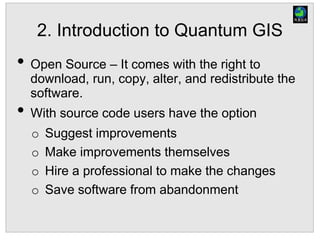
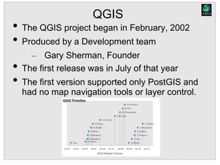
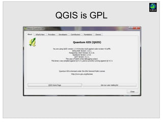
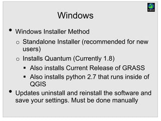
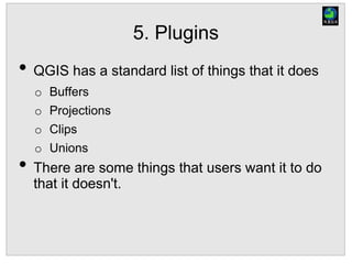
SlideShare a Scribd company logo
1 of 134
Introduction to Quantum GIS
• http://www.qgis.org
• http://www.osgeo.org
Agenda
• Overview of GIS
• Introduction to Quantum GIS
• Vector Data
• Raster Data
• Plugins
• Fields and Attribution
• Creating Data
• Map Layout
1. Overview of GIS
• Geographic Information System
• Wikipedia definition - it is a system designed to
capture, store, manipulate, analyze, manage,
and present all types of geographically
referenced data.
• It is used in many applications: Small
municipalities, forestry, military, commercial
businesses, etc., etc.,
• What do you do with it?
GIS
• Easily measure distances
• Easily measure areas
• Find overlap between features
• Proximity
• Everything is related by location.
o Tobler's Law
USGS Earthquake Zones
http://earthquake.usgs.gov
Simple Maps
Outputs from a GIS
• Maps
o Printed
• Digital (PDF, JPEG
• Spreadsheets
• Databases
• Files
o Shapefiles
o KML
2. Introduction to Quantum GIS
• Open Source – It comes with the right to
download, run, copy, alter, and redistribute the
software.
• With source code users have the option
o Suggest improvements
o Make improvements themselves
o Hire a professional to make the changes
o Save software from abandonment
Common OS Licensing
• Licenses to run in both open and proprietary
systems
o Apache Software License
o BSD (Berkeley Software Distribution)
o MIT (Massachusetts Institute of Technology)
• License to run in open environments
o GPL (General Public License)
o LPGL (Lesser General Public License)
o MPL (Mozilla Public License)
QGIS
• The QGIS project began in February, 2002
• Produced by a Development team
– Gary Sherman, Founder
• The first release was in July of that year
• The first version supported only PostGIS and
had no map navigation tools or layer control.
QGIS is GPL
Installing Quantum
• http://www.qgis.org
• I am going to stick with Windows and Linux
Installs.
– OSX - http://www.kyngchaos.com/software/qgis
• Linux – depending on your distribution of choice
you'll have a Debian or RPM install.
o Most systems with a large user base have
a GIS repository
o Ubuntu, Debian, Fedora
Windows
• Windows Installer Method
o Standalone Installer (recommended for new
users)
o Installs Quantum (Currently 1.8)
 Also installs Current Release of GRASS
 Also installs python 2.7 that runs inside of
QGIS
• Updates uninstall and reinstall the software and
save your settings. Must be done manually
Windows Installer cont'
• Standalone Method
o Geographic Data Abstraction Library
o Installs libraries for SID and ECW
o SID and ECW are proprietary formats that
have special agreements to be used with
GDAL
o http://www.gdal.org/
OSGEO Install
• OSGeo provides an installer that provides
everything.
o Runs in a “cygwin” type environment
o Cygwin provides unix commands and
environments on windows machines.
o Provides a means to an easy(ier) upgrade
path between releases.
o Isn't “installed” on your computer.
OSGEO Installer Cont'
• Quantum GIS
• GDAL
• GRASS
• OpenEV
• And UDIG (a great
data viewer).
3. Quantum GIS Interface
Layer Window
Map Canvas
Menus and Toolbars
Toolbars and Panels
• Right Click in
menu Area
• Add Panels
• Add
Toolbars.
Status Bar
• Projection of
the QGIS
project
• Scale
• Coordinates
Basic Buttons
• Hover mouse over them they will pop up a text message telling
the user their purpose.
• Add vector Layer
• Add Raster Layer
• PostGIS Layer
• Spatialite Layer
• WMS Layer
• New Shapefile Layer
• Remove Layer
• Oracle Raster Layer
• WFS Layer
• Pan
• Zoom In
• Zoom Out
• Pixel Resolution
• Zoom to Extent
• Zoom to Selection
• Zoom to Layer
• Zoom to Last Extent
• Zoom to Previous Extent
• Refresh
Attribution, Selection,
Measurements
• Identify
• Select
• Deselect
• Attribute Table
• Measure
• Maptips
•Add BookMark
•Show Bookmark
•Annotation
Saving a Project
• As you are working with QGIS periodically save
your datasets.
• QGIS creates a .gqs file
• XML based
• Can be edited in your favorite text editor.
Exercises
• Open QGIS
• Explore the Toolbars.
• Add some data to the Map Display
• Use the Identify Features tool to show attribute
to some data layers.
Exercise 2
The Exercises are going to be an actual project completed by North River Geographic Systems,
Inc in 2009. We are going to cover the Conasauga River Watershed. The watershed is located on
the border of Tennessee and Georgia. The data is made up of ESRI Shapefiles. That is the
easiest data format to work with for these exercises.
1. If you haven't already, open QGIS. There should be an icon on your desktop or on your start menu
(or both).
Once QGIS has opened right click with your mouse in the toolbar area.
How Many Toolbars are in the Default Installation
How many Panels are in the default Installation?
Turn off your Managed Layers toolbar. Turn Off your Map Navigation Toolbar. They have disappeared
from the interface. Now turn them back on. If you want you can move them from their default
location by grabbing the left corner of the toolbar and moving it.
2. Turn your Layers Panel off. Now turn it on by navigating from the View Menu at the top of QGIS
3. Click your Add Vector Data button at the top. Browse to your data folder located under
c:gisdataQGIStrainingdata . Add the CountyBoundaries.shp shapefile to your map. If you do
not see any data please be sure to check that you are adding shapefiles.
4. Click your add vector data button at the top and add the subbasin.shp file. You should have something
that looks like:
5. Using your identify features tool list all the counties in Georgia and the Counties in Tennessee. In order
to identify a feature you must have that layer selected in your layer window.
Georgia Tennessee
8. Click on the Subbasin shapefile in your Layers Panel and zoom to
the extent of that layer. Note you have several ways to make a
selection.
9. Select Whitfield County. Zoom to the extent of the selection.
10. Clear the selection.
11. Save your project in the Exercise 2 Directory!
6. Add the 2010 Urban Areas Shapefile.
What is the biggest Urban Area within the CountyBoundaries Shapefile?
What are the three biggest Urban Areas that touch/are within the Watershed?
7. Using your navigation tools Zoom to the full extent of all the data layers. You should see something similiar
to the graphic below.
3. Adding Vector Data
• Supports OGR vector Formats
o Shapefiles
o KML
o CSV
o Microstation
o MapINFO
Adding Vector Data
Properties
• Once Data is added – Right Click and Select
Properties
• There are different Tabs to help with Vector
Data
o Style, Label, Fields, General, Metadata,
Action Joins, Digrams, Overlay
o Style sets the symbology of the Layer.
o Symbology can be saved as a qml file
Transparency
Style
Styles
• Set by Fields
• Symbolized
o Single
o Categorized
o Graduated
• Graduated
o Equal Interval, Quantile, Natural Breaks,
Standard Deviation, Pretty Breaks
Equal Interval
• Equal Interval groups values into equal sized
ranges.
Quantile
• Each class contains an equal number of
features
Natural Breaks
• Natural Breaks classes are based on natural
groupings of the data.
Standard Deviation
• Show Variation from the average value
Pretty Breaks
• Data symbolized for non-statisticians
Labels
Selecting Vector Data
• Selections can be manual
Selecting Vector Data
• Selections can be by Attributes
• Selections can also be by location (Under
Vector Menu - Research)
Exercises
• Change the symbology of displayed data
• Label features
• Add a layer and categorize data by that item.
Exercise Ch 3
It's time to start looking at your data and working with it.. Most of the data you will be working with was
downloaded from the Census Bureau, the National Hydro Dataset, and the USDA DataGateway. Some
of these datasets were built by me during the course of the CRA project.
1. Add the Watershed.shp file to the Map Display.
2. How many main watersheds are located in
the Conasauga Watershed.
___________________
BONUS: Why is the Coahulla (pronounced Koa-
hull-ahhhh) split into a north and south section?
You might need to add more shapefiles to
answer this.
3. Label the Watersheds by name on the map
display. Rick click on the shapefile layer and
select properties. Select the labeling tab. Check
"Display Labels". Under Basic Label Options
pick Hu_10_Name
4. Right click on the watershed shapefile and go to properties. Look at the Style tab
5. Change the style of the data layer. Make
the polygon fill clear and the outline color
orange.
4. Right click on the watershed shapefile and go to properties. Look at the Style tab
5. Change the style of the data layer. Make
the polygon fill clear and the outline color
orange.
6. Save the Style. Right click on the watershed shapefile and click Save Style.
Save the file as a .qml file.
7. Once you have saved it remove the watershed shapefile by right clicking on it and selecting remove. Add it
again. Right click and select Load Style. Load the qml file you just saved. All of your original settings for this
layer have been restored.
8. Select North Coahulla using the select tool.
9. Right click and select “Save Selection As”. You have just saved the North Coahulla section of the
watershed.
10. Right click watershed.shp and open the Attribute table. We haven't covered this part yet in the class but
it's good to know for the purposes of the exercise.
11. Toggle editing on the attribute
layer. The Toggle editing Toolbar is
a small icon with a pencil located at
the bottom of the Attribute Window.
12. Add a field (add a new column) called Acres. Make sure it is a Decimal number
13. Once it has been added open the Field
Calculator. It is the last Icon at the bottom of the
Attribute Table Menu.
14. Click Update existing field. Under the function list select geometry and double click $area. Add
/43560 in the Expression area. Click OK.
15. Right Click the watershed Layer. Go to Properties. Click the style Tab. Change the symbology to
Categorized by acres. Click Classify at the bottom left of the menu. Click OK.
16. You have just calculated the Acreage of each watershed. What is the biggest watershed? What is the total
size in acres of the Watershed? (HINT Vector Menu → Analysis Tools → Basic Statistics.
4. Adding Raster Data
• Supports OGR Raster Formats
o Geotiff
o ESRi Grid
o Jpeg
• Sid & ECW Format
o Read and not write the format
o Support must be added
o Included with standalone installer
Geospatial Data Abstraction Library
• Approximately 128 Formats supported
o http://www.gdal.org
• Many command line tools
o Convert
o Reproject
o Warp
o Mosaic
WMS – WFS Standards
• Web mapping service - The OpenGIS Web Map Service
Interface Standard (WMS) provides a simple HTTP interface for
requesting geo-registered map images from one or more
distributed geospatial databases.
• Web Feature Service - Web Feature Service Interface Standard
(WFS) provides an interface allowing requests for geographical
features across the web using platform-independent calls
WMS Example
http://raster.nationalmap.gov/ArcGIS/services/DRG/TNM_Digi
tal_Raster_Graphics/MapServer/WMSServer?request=Get
Capabilities&service=WMS
WMS Example
Exercises
• Add raster data
• Symbolize Raster Data
• Create a Hillshaded DEM
Exercise Chapter 4
1. Add the Watershed.shp file to the Map Display.
2. Add the tif image of Whitfield County to the display. The image name is whitfield_naip_tiled_2009.tif
3. Right Click the image layer and select rename. Name it “Whitfield County 2009” . Note that it added to top of
your layer window. Last thing added gets placed on top of the layers.
4. Right click the Whitfield County 2009 layer and go to properties. Set the transparency at 40%.
5. Set the Transparency back to
0%
6. Look to the right and set the “No data
value” to 0. Click OK.
7. What was the result?
Since this project deals with watersheds you will want to add a digital Elevation model to this project. One was
downloaded from http://seamless.usgs.gov. It is an ESRI grid Format.
Add the file float35w085_1.flt from the ElevationModel directory to your display. Note that it is an ESRI Grid
format.You will need to use the “Add Raster” button to add the DEM
8. Right click on the DEM and go to Properties. Click on the style tab. Change the contrast enhancement to Stretch
to Min Max.
9. You should now see an image that covers the extent of Murray County and also covers a major portion of the
watershed. Make the Watershed Transparent. Use the identify features tool to identify elevations on the DEM.
10. Go to the Raster Menu at the top of QGIS. Click on Analysis and then DEM (terrain Models). There is one thing
we will need to change before running this command. We will need to set the scale.
Scale is the ration of vertical units to horizontal. Since the DEM is in a geographic Projection and has vertical units
in meters scale will need to be set. If the horizontal unit of the source DEM is degrees (WGS84), you can use
scale=111120 if the vertical units are meters or scale=370400 if they are in feet.
11. On the DEM menu name an output file. Make sure the mode is set to hillshade. Make sure the scale is set to
111120.00 . Before clicking OK make sure the Load onto Canvas checkbox is checked.
12. Inspect the hillshaded DEM. Once you are happy save
your exercise!
5. Plugins
• QGIS has a standard list of things that it does
o Buffers
o Projections
o Clips
o Unions
• There are some things that users want it to do
that it doesn't.
Fetching Plugins
Plugin Interface
Add Plugins from the Filter Text Box
Official Plugins and 3rd Party
Plugins
Community approves plugins
Manage Plugins
• You can add and remove plugins through the
QGIS Plugin Manager
• Plugins I have used
o Grass
o GDAL Tools
o OpenStreetMap Plugin
o Sextante Plugin
QGIS Plugins 3rd Party
• Use at your own risk
• They can be poorly documented and in may
cases not work
• Developers may build plugin for certain
platforms
o Home Range Plugin runs on Linux and not on
windows
o Developer can be paid to make/fix plugins
o Overall – plugins are awesome.
Exercises
• Explore Plugins and plugins manager
• Work with OpenLayers
• Look at Sextante
While you're working on a project you might need access to more functionality. QGIS does a lot, Plugins allow you
to do more.
1. Click on the plugins menu at the top of QGIS. Notice you have several choices under the main menu for plugins
into QGIS. Python being one of them. Grass being another. Click on the start button in windows and drive to the
QGIS folder under installed programs (Programs (x86)). Notice that Grass is installed under the QGIS Folder. What
is Grass and how long has it been around? (You can use Google!)
2. Open the QGIS plugin manager. How many default plugins are available to QGIS?
3. Open the QGIS Fetch Python Plugins Menu. How many plugins are available? (acceptable answer can be A Lot
)
Exercise Chapter 5
4. Install the OpenLayers Plugin.
5. Once installed go back to the plugins menu and add the
OpenLayers Overview.
6. Add the Watershed Layer to QGIS.
7. On the OpenLayers plugin enable the Google Satellite view.
8. Click the add Map icon on the OpenLayers plugin.
9. Add the Sextante plugin. Notice when it is added you will have an Analysis Menu added to the QGIS Interface.
What is Sextante? What other software package can use Sextante?
10. Add the Sextante Toolbox.
11. Once you are done looking at the plugins, close QGIS!
6. Attributes
• GIS is more than just Geometry – there are
attributes built into the data.
Attribution depends on the database
• We are using Shapefiles
• It also reads PostGIS, SQL Server, ESRI's
SDE, Spatialite, etc, etc.
• Pay Attention to Spatialite.
– http://www.gaia-gis.it/gaia-sins/
Search for Attributes
• As an example a user needs to search for
houses
Selecting based on Attribute
• Note search was on a text field and was not “Quoted”
• Selection set can be saved to a new shapefile file
• Selection set can be saved to the clipboard/excel/notepad
Selections are reflected in the
Display
Advanced Search
• SQL Query
Add and Columns
• Data layer must be editable
• Right click on a data layer and Toggle Editing
• Toggle editing under the Layer Menu
• Toggle Editing from Attribute Menu
Deleting Columns
• Toggle Editing
• Click Delete Columns Icon
Calculate Area
• Add Column and use the area calculation in the
Field Calculator
Exercises
• Add and Delete Fields
• Calculate Field Values
• Select data by attributes
1. Open QGIS and add the Watershed layer to your display. Open the attribute table by right clicking on the layer
and clicking “Open Attribute Table”.
2. You need to calculate the square miles of each watershed. Toggle Editing.
Exercise Ch 6
3. Add a column by clicking on the add column icon. Atributtes for the new column depend on the
database format being used. In this case we are using dbase (dbf). Make your new column name
sqmiles. Make the Type decimal number. Make the width 6 and the precision (number of decimal
places) 4.
4. Since this shapefile is in Georgia West
Stateplane NAD 83 US Feet (Projections are
coming in a bit), The important thing to know
is the Area (Shape_Area) is in Square
Feet. There are 640 Acres in a Square Mile.
A. Open the field Calculator. If “Only update
selected features” is checked, uncheck it.
B. Check update existing field. Select square
miles from the combo both.
C. In the left hand box labeled Function List Click
Fields and Values and then double click
Acres. Double clicking adds it to the
expression box at the bottom.
D. Click the division symbol.
E. Type 640 . See if what you have looks like the
figure to the Right:
F. Click OK. Click the editing icon and save your edits. Congratulations. You've just calculated Acres
for the watershed.
5. Add the Streams shapefile to QGIS. This data came from the National Hydro Dataset and has had
more attributes added to it. The Conasauga River is the main River that flows through the watershed.
Open the attribute table and search for the Conasauga River using the GNIS_Name as the search
field. Type in Conasauga.
Click the Show Selected Only. Notice it did a wild card search by default and looked for the word
“Conasauga” in the results. Some results are showing Conasauga Creek while others are showing
Conasauga River. Notice the Creek to the north west of the main river.
6. Now we're going to build an
SQL Statement using Advanced
Search. Click Advanced Search.
A. Double Click GNIS_Name
under fields
B. Click the = Sign
C. Under Values Click All.
D. Double Click 'Conasauga
River'
E. Check your expression.
F. Click OK.
7. Now that you have selected the main stem of the Conasauga River, unselect it using the Unselect
Icon on the Attribute table.
8. Remove the following attributes from the Shapefile: Enabled, From_Node, To_Node, fromelev,
ToElev. You will have to enable editing and then click the Delete Column icon.
9. Once you have finished, Stop editing by clicking the Editing icon located on the Attribute Menu. You
will be prompted to save your edits.
7. Creating new Data and Editing
• You can create new types of data in QGIS
o Shapefiles
o Spatialite Layer
• Layers contain basic Geometry shapes
o Points
o Lines
o Polygons
Map Projections
• Geographic Coordinate Systems
o Defines locations on spherical model of the earth
• Projected Coordinate System
o Defines locations on flat model of the earth
Geographic Coordinate System
• Defines Locations with Latitude Longitude
Values
o Latitude – north and south of the equator
o Longitude - east and west of prime meridian
o Prime meridian is Greenwich
Projected Coordinate System
• Define Locations with map
units
o X and Y measured from a
Origin
o Projected Coordinate
system includes
o Units in feet or meters
o A Map Projection
o Underlying Geographic
Coordinate System
EPSG Geodetic Parameter Registry
• Gatekeepers of Projections
• Also knows as SRIDS (Spatial Reference
System Identifier)
• http://www.epsg-registry.org/
Create a new shapefile
EPSG:4326
• QGIS has 4326 as a Default Projection
– Which is WGS 84
• It can be changed
Define the Properties of the
Shapefile
• Points, Lines, or Polygons
• Projection ( Coordinate
Reference System)
• Attribution
o Text
o Whole Number
o Decimal Number
Spatialite
• You can make a spatialite layer
o Very "similar" to ESRI's Geodatabase Format
o All files are kept in one file/database
o Can be accessed from a number of softwares
 QGIS
 Python
 GDAL
 Mapnik
• Cannot be accessed by ESRI Software.....yet.
Editing Data
• Once data is created or
added to the Map View it
can be edited two different
ways
• Right click on the layer
and Toggle Editing
• Go to layer menu and
Toggle Editing
Editing Menus
• From Left to Right
o Toggle Editing
o Save Edits
o Capture Feature (in this case polygon)
o Create and move nodes
o Delete Feature
o Cut Feature
o Copy Feature
o Past Feature
Advanced Editing
• From left to right
o Undo
o Redo
o Simplify
o Add ring
o Add part (multi-feature)
o Delete Ring
o Delete Part
o Reshape Feature
o Split
o Merge Features
o Merge Attributes
o Rotate Point Symbols
Editing
• Note – When you start editing the feature
changes on the Editing Toolbar
• Example Editing Points:
Multiple layers can be edited at
once
• Example: I need to edit both points and lines
o Select Dataset
o Begin Editing
Once a feature is placed: Attribution
• Immediately upon adding a feature you attribute
it.
Snapping
• Added features can be snapped to vertex or
segment (edge)
• Located under Settings → Snapping Options
Attribution
• Attribution can be controlled
if you have thought out your
GIS data input.
• Ranges and Lists can be
generated for user input very
easily.
o Known as an edit widget
o It is found under Layer
Properties
Example
• Value Map for the field “Descriptio”
Once you set a Value Map
• Pick List
Exercises
• Edit data
• Create points and polygons
• Delete Data
• Create an input widget
Exercise 7
Time to start editing. We need to edit some of the vector data to match the raster data.
1. Open exercise 7-.qgs under the Editing directory. Now – when the .qgs project is opened something fun might
happen. If the project hasn't been set up with relative path names you might have to reset the project.
2. A utility company has added a storage
pond. The digital data doesn't reflect that
storage pond. There are three streams that
don't belong and at least two ponds. So you
need to delete the two ponds that fall within
the storage pond and add the storage pond.
3. Right click NHDWaterbody and Toggle
Editing.
4. Using your Select Single feature Tool
select the pond that falls withing the storage
facility and delete it. There are at least two
ways to delete this feature. What are
they?
5. Delete the second pond that appears on the north east side of the Storage Pond. Delete the stream segments
that touch the storage pond.
6. Using the add features icon add the storage pond.
7. Once you finish tracing the pond right click your mouse. You will be prompted to fill in the attributes. Don't worry
about filling anything out. Save your edits.
8. Click "Toggle Editing" to stop editing.
9. Save and close Exercise7-1
10. Open Exercise7-2.
11. You need to identify houses in this study
area. The study area shown to the right is
missing. You can create a new study
area of interpret from the image. There is
a problem with fecal coliform
contamination in the streams. There will
be 5 types of structures present in the
watershed:
• Houses
• Commercial
• Barns
• Agricultural
• Mobile Homes
12. You need to create a shapefile to store
points. Each structure in this area will get
one point as close to the center of the
structure as you can.
13. Click on the layer menu and create a new shapefile. Specify the CRS to be Georgia West - NAD83
(ftUS). Add one text attribute called "Name" and make it text with a width of 24. Save the file and
call it structures_point.shp in your data directory.
14. Toggle Editing "on" for the structures
Shapefile. Start adding points. Notice that after
each point is added it prompts you to fill out
the attributes. Be sure to label each point as a
House, Agriculture, Mobile Home,
Commercial, or Barn. Put in about 15 or 20
points. Save. Stop Editing
15. Right click the structures_point.shp and open the properties. Click on the fields tab.
16. Click the Line edit Button under
Edit Widget. This give you the
ability to add dropdown lists.
Select "Value Map" and add 5
attributes:
• Home
• Mobile Home
• Commercial
• Agriculture
• Barns
17. Edit the structures shapefile and
start putting a point on top of
the structures. Notice the drop
down list
8. Map Layout
• The Map view can be exported with Map
Composer.
o Composer Manager
 Multiple Map compositions can be stored.
• Map compositions can be exported to several
different file formats
o PDF
o JPG
o TIFF
New Composition
• File → New Print Composer
Map Composer
• Map Compositions can be saved (as a
Template)
• Templates can be applied to new Map
Compositions
• Compositions can have legend, Pictures, Scale
bar.
Toolbar for Map Composer
• Open
• Save
• Export to image
• Export to PDF
• Export to SVG
• Print
• Refresh
• Undo
• Redo
• Add map
• Add image
• Add label
• From left to right
•Add Scale
•Add Shape
•Add Arrow
•Move Item
•Move Content
•Group Items
•Ungroup Items
• Raise Selected Items
•Add legend
•Align Selected Items
Page Size
• Page options can be
set
o Standard Sizes
o Custom Sizes
o Resolution
o Landscape/Portrait
o Grid for drawing
features
Adding Map Element
• Scale
• Draw
Extents
• Rotation
Map Elements
• Can be added to your map
o Pictures: logos or camera shots
o North Arrow (needs to be custom)
o Legend (can be customized
• There is an undo button and redo button so you
can back up.
Legend
• Can be customized
• Items can be removed
o Imagery
o Base maps that do not need a legend
o Text can be added next to layer symbology
Export and Print
• Can be exported as Image, PDF, SVG
• Can then be imported into another program
o GIMP
o Adobe Photoshop or Adobe Illustrator
o InkScape
Exercises
• Group Exercise
• Make a map
• Explore Print Composer
Exercise Ch 8
....and you're almost done. Time for the fun stuff. You need to make a map. There will be no
screenshots of a map. This one is all up to you.
1. Open QGIS.
2. Add the following shapefiles: Watershed Streams, NHDArea, and NHDWaterbody.
3. Go to the File Menu and click on New Print Composer.
4. Set the Page size for your Map.
5. Click the Add a new map icon and add a new map by dragging a box on your page.
6. Once it has been added click on Item Properties and set a Map
Scale and adjust the width and height of your new map item.
7. Add a legend by clicking the legend icon and clicking on your
page. Notice how you can customize the Legend by looking at
the item properties.
8. Notice you can group, ungroup, and align certain items. You can
also add labels.
9. Click on File in the upper left hand corner and look at your export
options.
10. Add an image and look at the pre-loaded images. You can add
a North Arrow and Sync that with the map. When you sync the
North Arrow it will turn if the map turns.
Conclusion
• It is possible to use Freely available GIS Tools
to complete small or big projects
o It's an active community – Join in
o http://www.qgis.org
o User Manual -
http://qgis.org/en/documentation/manuals.html
o Wiki - http://qgis.org/en/community.html
Contributors
• Randal Hale – North River Geographic
Systems, Inc
• Carol Kraemer – North River Geographic
Systems, Inc

More Related Content

Similar to Introduction_to_QGIS_Revision, read before

Watershed Delineation Using ArcMap
Watershed Delineation Using ArcMapWatershed Delineation Using ArcMap
Watershed Delineation Using ArcMapArthur Green
 
Crystal tr///SAP Design Studio online training by design studio Export-24/7//...
Crystal tr///SAP Design Studio online training by design studio Export-24/7//...Crystal tr///SAP Design Studio online training by design studio Export-24/7//...
Crystal tr///SAP Design Studio online training by design studio Export-24/7//...venkat training
 
Mapping Immigrants
Mapping ImmigrantsMapping Immigrants
Mapping Immigrantsborderzine
 
SAGT Conference 2016 - Teaching Census through GIS
SAGT Conference 2016 - Teaching Census through GISSAGT Conference 2016 - Teaching Census through GIS
SAGT Conference 2016 - Teaching Census through GISceliamac58
 
GeoSDI: una piattaforma social di dati geografici basata sui principi di INSP...
GeoSDI: una piattaforma social di dati geografici basata sui principi di INSP...GeoSDI: una piattaforma social di dati geografici basata sui principi di INSP...
GeoSDI: una piattaforma social di dati geografici basata sui principi di INSP...Beniamino Murgante
 
Global mapper tutorial Jimma University Ethiopia
Global mapper tutorial Jimma University EthiopiaGlobal mapper tutorial Jimma University Ethiopia
Global mapper tutorial Jimma University Ethiopiachala hailu
 
Integrating PostGIS in Web Applications
Integrating PostGIS in Web ApplicationsIntegrating PostGIS in Web Applications
Integrating PostGIS in Web ApplicationsCommand Prompt., Inc
 
MapInfo Professional 12.5 and Discover3D 2014 - A brief overview
MapInfo Professional 12.5 and Discover3D 2014 - A brief overviewMapInfo Professional 12.5 and Discover3D 2014 - A brief overview
MapInfo Professional 12.5 and Discover3D 2014 - A brief overviewPrakher Hajela Saxena
 
Going Mobile with HTML5
Going Mobile with HTML5Going Mobile with HTML5
Going Mobile with HTML5John Reiser
 
Geographic information system and remote sensing
Geographic information system and remote sensingGeographic information system and remote sensing
Geographic information system and remote sensingchala hailu
 
Cutter et al-2007-Systematic Conservation Planning Module
Cutter et al-2007-Systematic Conservation Planning ModuleCutter et al-2007-Systematic Conservation Planning Module
Cutter et al-2007-Systematic Conservation Planning ModulePeter Cutter
 
GR2-12_DivaGIS_metod.pptx
GR2-12_DivaGIS_metod.pptxGR2-12_DivaGIS_metod.pptx
GR2-12_DivaGIS_metod.pptxPaúl Gonzáles
 

Similar to Introduction_to_QGIS_Revision, read before (20)

manual global mapper
manual global mappermanual global mapper
manual global mapper
 
Watershed Delineation Using ArcMap
Watershed Delineation Using ArcMapWatershed Delineation Using ArcMap
Watershed Delineation Using ArcMap
 
Global mapperhelp
Global mapperhelpGlobal mapperhelp
Global mapperhelp
 
Crystal tr///SAP Design Studio online training by design studio Export-24/7//...
Crystal tr///SAP Design Studio online training by design studio Export-24/7//...Crystal tr///SAP Design Studio online training by design studio Export-24/7//...
Crystal tr///SAP Design Studio online training by design studio Export-24/7//...
 
Mapping Immigrants
Mapping ImmigrantsMapping Immigrants
Mapping Immigrants
 
SAGT Conference 2016 - Teaching Census through GIS
SAGT Conference 2016 - Teaching Census through GISSAGT Conference 2016 - Teaching Census through GIS
SAGT Conference 2016 - Teaching Census through GIS
 
Global mapperhelp
Global mapperhelpGlobal mapperhelp
Global mapperhelp
 
GeoSDI: una piattaforma social di dati geografici basata sui principi di INSP...
GeoSDI: una piattaforma social di dati geografici basata sui principi di INSP...GeoSDI: una piattaforma social di dati geografici basata sui principi di INSP...
GeoSDI: una piattaforma social di dati geografici basata sui principi di INSP...
 
Global mapper tutorial Jimma University Ethiopia
Global mapper tutorial Jimma University EthiopiaGlobal mapper tutorial Jimma University Ethiopia
Global mapper tutorial Jimma University Ethiopia
 
Rpsonmongodb
RpsonmongodbRpsonmongodb
Rpsonmongodb
 
Integrating PostGIS in Web Applications
Integrating PostGIS in Web ApplicationsIntegrating PostGIS in Web Applications
Integrating PostGIS in Web Applications
 
Q GIS Training Presentation
Q GIS Training PresentationQ GIS Training Presentation
Q GIS Training Presentation
 
MapInfo Professional 12.5 and Discover3D 2014 - A brief overview
MapInfo Professional 12.5 and Discover3D 2014 - A brief overviewMapInfo Professional 12.5 and Discover3D 2014 - A brief overview
MapInfo Professional 12.5 and Discover3D 2014 - A brief overview
 
Big data
Big dataBig data
Big data
 
Going Mobile with HTML5
Going Mobile with HTML5Going Mobile with HTML5
Going Mobile with HTML5
 
Big data
Big dataBig data
Big data
 
Geohosting
GeohostingGeohosting
Geohosting
 
Geographic information system and remote sensing
Geographic information system and remote sensingGeographic information system and remote sensing
Geographic information system and remote sensing
 
Cutter et al-2007-Systematic Conservation Planning Module
Cutter et al-2007-Systematic Conservation Planning ModuleCutter et al-2007-Systematic Conservation Planning Module
Cutter et al-2007-Systematic Conservation Planning Module
 
GR2-12_DivaGIS_metod.pptx
GR2-12_DivaGIS_metod.pptxGR2-12_DivaGIS_metod.pptx
GR2-12_DivaGIS_metod.pptx
 

Recently uploaded

Customer Service Analytics - Make Sense of All Your Data.pptx
Customer Service Analytics - Make Sense of All Your Data.pptxCustomer Service Analytics - Make Sense of All Your Data.pptx
Customer Service Analytics - Make Sense of All Your Data.pptxEmmanuel Dauda
 
Predicting Employee Churn: A Data-Driven Approach Project Presentation
Predicting Employee Churn: A Data-Driven Approach Project PresentationPredicting Employee Churn: A Data-Driven Approach Project Presentation
Predicting Employee Churn: A Data-Driven Approach Project PresentationBoston Institute of Analytics
 
Brighton SEO | April 2024 | Data Storytelling
Brighton SEO | April 2024 | Data StorytellingBrighton SEO | April 2024 | Data Storytelling
Brighton SEO | April 2024 | Data StorytellingNeil Barnes
 
Industrialised data - the key to AI success.pdf
Industrialised data - the key to AI success.pdfIndustrialised data - the key to AI success.pdf
Industrialised data - the key to AI success.pdfLars Albertsson
 
RA-11058_IRR-COMPRESS Do 198 series of 1998
RA-11058_IRR-COMPRESS Do 198 series of 1998RA-11058_IRR-COMPRESS Do 198 series of 1998
RA-11058_IRR-COMPRESS Do 198 series of 1998YohFuh
 
VIP Call Girls Service Miyapur Hyderabad Call +91-8250192130
VIP Call Girls Service Miyapur Hyderabad Call +91-8250192130VIP Call Girls Service Miyapur Hyderabad Call +91-8250192130
VIP Call Girls Service Miyapur Hyderabad Call +91-8250192130Suhani Kapoor
 
Indian Call Girls in Abu Dhabi O5286O24O8 Call Girls in Abu Dhabi By Independ...
Indian Call Girls in Abu Dhabi O5286O24O8 Call Girls in Abu Dhabi By Independ...Indian Call Girls in Abu Dhabi O5286O24O8 Call Girls in Abu Dhabi By Independ...
Indian Call Girls in Abu Dhabi O5286O24O8 Call Girls in Abu Dhabi By Independ...dajasot375
 
Call Girls in Defence Colony Delhi 💯Call Us 🔝8264348440🔝
Call Girls in Defence Colony Delhi 💯Call Us 🔝8264348440🔝Call Girls in Defence Colony Delhi 💯Call Us 🔝8264348440🔝
Call Girls in Defence Colony Delhi 💯Call Us 🔝8264348440🔝soniya singh
 
04242024_CCC TUG_Joins and Relationships
04242024_CCC TUG_Joins and Relationships04242024_CCC TUG_Joins and Relationships
04242024_CCC TUG_Joins and Relationshipsccctableauusergroup
 
Beautiful Sapna Vip Call Girls Hauz Khas 9711199012 Call /Whatsapps
Beautiful Sapna Vip  Call Girls Hauz Khas 9711199012 Call /WhatsappsBeautiful Sapna Vip  Call Girls Hauz Khas 9711199012 Call /Whatsapps
Beautiful Sapna Vip Call Girls Hauz Khas 9711199012 Call /Whatsappssapnasaifi408
 
꧁❤ Greater Noida Call Girls Delhi ❤꧂ 9711199171 ☎️ Hard And Sexy Vip Call
꧁❤ Greater Noida Call Girls Delhi ❤꧂ 9711199171 ☎️ Hard And Sexy Vip Call꧁❤ Greater Noida Call Girls Delhi ❤꧂ 9711199171 ☎️ Hard And Sexy Vip Call
꧁❤ Greater Noida Call Girls Delhi ❤꧂ 9711199171 ☎️ Hard And Sexy Vip Callshivangimorya083
 
VIP Call Girls in Amravati Aarohi 8250192130 Independent Escort Service Amravati
VIP Call Girls in Amravati Aarohi 8250192130 Independent Escort Service AmravatiVIP Call Girls in Amravati Aarohi 8250192130 Independent Escort Service Amravati
VIP Call Girls in Amravati Aarohi 8250192130 Independent Escort Service AmravatiSuhani Kapoor
 
EMERCE - 2024 - AMSTERDAM - CROSS-PLATFORM TRACKING WITH GOOGLE ANALYTICS.pptx
EMERCE - 2024 - AMSTERDAM - CROSS-PLATFORM  TRACKING WITH GOOGLE ANALYTICS.pptxEMERCE - 2024 - AMSTERDAM - CROSS-PLATFORM  TRACKING WITH GOOGLE ANALYTICS.pptx
EMERCE - 2024 - AMSTERDAM - CROSS-PLATFORM TRACKING WITH GOOGLE ANALYTICS.pptxthyngster
 
Building on a FAIRly Strong Foundation to Connect Academic Research to Transl...
Building on a FAIRly Strong Foundation to Connect Academic Research to Transl...Building on a FAIRly Strong Foundation to Connect Academic Research to Transl...
Building on a FAIRly Strong Foundation to Connect Academic Research to Transl...Jack DiGiovanna
 
FESE Capital Markets Fact Sheet 2024 Q1.pdf
FESE Capital Markets Fact Sheet 2024 Q1.pdfFESE Capital Markets Fact Sheet 2024 Q1.pdf
FESE Capital Markets Fact Sheet 2024 Q1.pdfMarinCaroMartnezBerg
 
Unveiling Insights: The Role of a Data Analyst
Unveiling Insights: The Role of a Data AnalystUnveiling Insights: The Role of a Data Analyst
Unveiling Insights: The Role of a Data AnalystSamantha Rae Coolbeth
 
Call Girls In Mahipalpur O9654467111 Escorts Service
Call Girls In Mahipalpur O9654467111  Escorts ServiceCall Girls In Mahipalpur O9654467111  Escorts Service
Call Girls In Mahipalpur O9654467111 Escorts ServiceSapana Sha
 

Recently uploaded (20)

Customer Service Analytics - Make Sense of All Your Data.pptx
Customer Service Analytics - Make Sense of All Your Data.pptxCustomer Service Analytics - Make Sense of All Your Data.pptx
Customer Service Analytics - Make Sense of All Your Data.pptx
 
Predicting Employee Churn: A Data-Driven Approach Project Presentation
Predicting Employee Churn: A Data-Driven Approach Project PresentationPredicting Employee Churn: A Data-Driven Approach Project Presentation
Predicting Employee Churn: A Data-Driven Approach Project Presentation
 
Delhi 99530 vip 56974 Genuine Escort Service Call Girls in Kishangarh
Delhi 99530 vip 56974 Genuine Escort Service Call Girls in  KishangarhDelhi 99530 vip 56974 Genuine Escort Service Call Girls in  Kishangarh
Delhi 99530 vip 56974 Genuine Escort Service Call Girls in Kishangarh
 
Brighton SEO | April 2024 | Data Storytelling
Brighton SEO | April 2024 | Data StorytellingBrighton SEO | April 2024 | Data Storytelling
Brighton SEO | April 2024 | Data Storytelling
 
Industrialised data - the key to AI success.pdf
Industrialised data - the key to AI success.pdfIndustrialised data - the key to AI success.pdf
Industrialised data - the key to AI success.pdf
 
RA-11058_IRR-COMPRESS Do 198 series of 1998
RA-11058_IRR-COMPRESS Do 198 series of 1998RA-11058_IRR-COMPRESS Do 198 series of 1998
RA-11058_IRR-COMPRESS Do 198 series of 1998
 
VIP Call Girls Service Miyapur Hyderabad Call +91-8250192130
VIP Call Girls Service Miyapur Hyderabad Call +91-8250192130VIP Call Girls Service Miyapur Hyderabad Call +91-8250192130
VIP Call Girls Service Miyapur Hyderabad Call +91-8250192130
 
Indian Call Girls in Abu Dhabi O5286O24O8 Call Girls in Abu Dhabi By Independ...
Indian Call Girls in Abu Dhabi O5286O24O8 Call Girls in Abu Dhabi By Independ...Indian Call Girls in Abu Dhabi O5286O24O8 Call Girls in Abu Dhabi By Independ...
Indian Call Girls in Abu Dhabi O5286O24O8 Call Girls in Abu Dhabi By Independ...
 
Call Girls in Defence Colony Delhi 💯Call Us 🔝8264348440🔝
Call Girls in Defence Colony Delhi 💯Call Us 🔝8264348440🔝Call Girls in Defence Colony Delhi 💯Call Us 🔝8264348440🔝
Call Girls in Defence Colony Delhi 💯Call Us 🔝8264348440🔝
 
04242024_CCC TUG_Joins and Relationships
04242024_CCC TUG_Joins and Relationships04242024_CCC TUG_Joins and Relationships
04242024_CCC TUG_Joins and Relationships
 
꧁❤ Aerocity Call Girls Service Aerocity Delhi ❤꧂ 9999965857 ☎️ Hard And Sexy ...
꧁❤ Aerocity Call Girls Service Aerocity Delhi ❤꧂ 9999965857 ☎️ Hard And Sexy ...꧁❤ Aerocity Call Girls Service Aerocity Delhi ❤꧂ 9999965857 ☎️ Hard And Sexy ...
꧁❤ Aerocity Call Girls Service Aerocity Delhi ❤꧂ 9999965857 ☎️ Hard And Sexy ...
 
Beautiful Sapna Vip Call Girls Hauz Khas 9711199012 Call /Whatsapps
Beautiful Sapna Vip  Call Girls Hauz Khas 9711199012 Call /WhatsappsBeautiful Sapna Vip  Call Girls Hauz Khas 9711199012 Call /Whatsapps
Beautiful Sapna Vip Call Girls Hauz Khas 9711199012 Call /Whatsapps
 
꧁❤ Greater Noida Call Girls Delhi ❤꧂ 9711199171 ☎️ Hard And Sexy Vip Call
꧁❤ Greater Noida Call Girls Delhi ❤꧂ 9711199171 ☎️ Hard And Sexy Vip Call꧁❤ Greater Noida Call Girls Delhi ❤꧂ 9711199171 ☎️ Hard And Sexy Vip Call
꧁❤ Greater Noida Call Girls Delhi ❤꧂ 9711199171 ☎️ Hard And Sexy Vip Call
 
VIP Call Girls in Amravati Aarohi 8250192130 Independent Escort Service Amravati
VIP Call Girls in Amravati Aarohi 8250192130 Independent Escort Service AmravatiVIP Call Girls in Amravati Aarohi 8250192130 Independent Escort Service Amravati
VIP Call Girls in Amravati Aarohi 8250192130 Independent Escort Service Amravati
 
EMERCE - 2024 - AMSTERDAM - CROSS-PLATFORM TRACKING WITH GOOGLE ANALYTICS.pptx
EMERCE - 2024 - AMSTERDAM - CROSS-PLATFORM  TRACKING WITH GOOGLE ANALYTICS.pptxEMERCE - 2024 - AMSTERDAM - CROSS-PLATFORM  TRACKING WITH GOOGLE ANALYTICS.pptx
EMERCE - 2024 - AMSTERDAM - CROSS-PLATFORM TRACKING WITH GOOGLE ANALYTICS.pptx
 
Building on a FAIRly Strong Foundation to Connect Academic Research to Transl...
Building on a FAIRly Strong Foundation to Connect Academic Research to Transl...Building on a FAIRly Strong Foundation to Connect Academic Research to Transl...
Building on a FAIRly Strong Foundation to Connect Academic Research to Transl...
 
FESE Capital Markets Fact Sheet 2024 Q1.pdf
FESE Capital Markets Fact Sheet 2024 Q1.pdfFESE Capital Markets Fact Sheet 2024 Q1.pdf
FESE Capital Markets Fact Sheet 2024 Q1.pdf
 
Unveiling Insights: The Role of a Data Analyst
Unveiling Insights: The Role of a Data AnalystUnveiling Insights: The Role of a Data Analyst
Unveiling Insights: The Role of a Data Analyst
 
Decoding Loan Approval: Predictive Modeling in Action
Decoding Loan Approval: Predictive Modeling in ActionDecoding Loan Approval: Predictive Modeling in Action
Decoding Loan Approval: Predictive Modeling in Action
 
Call Girls In Mahipalpur O9654467111 Escorts Service
Call Girls In Mahipalpur O9654467111  Escorts ServiceCall Girls In Mahipalpur O9654467111  Escorts Service
Call Girls In Mahipalpur O9654467111 Escorts Service
 

Introduction_to_QGIS_Revision, read before

  • 1. Introduction to Quantum GIS • http://www.qgis.org • http://www.osgeo.org
  • 2. Agenda • Overview of GIS • Introduction to Quantum GIS • Vector Data • Raster Data • Plugins • Fields and Attribution • Creating Data • Map Layout
  • 3. 1. Overview of GIS • Geographic Information System • Wikipedia definition - it is a system designed to capture, store, manipulate, analyze, manage, and present all types of geographically referenced data. • It is used in many applications: Small municipalities, forestry, military, commercial businesses, etc., etc., • What do you do with it?
  • 4. GIS • Easily measure distances • Easily measure areas • Find overlap between features • Proximity • Everything is related by location. o Tobler's Law
  • 7. Outputs from a GIS • Maps o Printed • Digital (PDF, JPEG • Spreadsheets • Databases • Files o Shapefiles o KML
  • 8. 2. Introduction to Quantum GIS • Open Source – It comes with the right to download, run, copy, alter, and redistribute the software. • With source code users have the option o Suggest improvements o Make improvements themselves o Hire a professional to make the changes o Save software from abandonment
  • 9. Common OS Licensing • Licenses to run in both open and proprietary systems o Apache Software License o BSD (Berkeley Software Distribution) o MIT (Massachusetts Institute of Technology) • License to run in open environments o GPL (General Public License) o LPGL (Lesser General Public License) o MPL (Mozilla Public License)
  • 10. QGIS • The QGIS project began in February, 2002 • Produced by a Development team – Gary Sherman, Founder • The first release was in July of that year • The first version supported only PostGIS and had no map navigation tools or layer control.
  • 12. Installing Quantum • http://www.qgis.org • I am going to stick with Windows and Linux Installs. – OSX - http://www.kyngchaos.com/software/qgis • Linux – depending on your distribution of choice you'll have a Debian or RPM install. o Most systems with a large user base have a GIS repository o Ubuntu, Debian, Fedora
  • 13. Windows • Windows Installer Method o Standalone Installer (recommended for new users) o Installs Quantum (Currently 1.8)  Also installs Current Release of GRASS  Also installs python 2.7 that runs inside of QGIS • Updates uninstall and reinstall the software and save your settings. Must be done manually
  • 14. Windows Installer cont' • Standalone Method o Geographic Data Abstraction Library o Installs libraries for SID and ECW o SID and ECW are proprietary formats that have special agreements to be used with GDAL o http://www.gdal.org/
  • 15. OSGEO Install • OSGeo provides an installer that provides everything. o Runs in a “cygwin” type environment o Cygwin provides unix commands and environments on windows machines. o Provides a means to an easy(ier) upgrade path between releases. o Isn't “installed” on your computer.
  • 16. OSGEO Installer Cont' • Quantum GIS • GDAL • GRASS • OpenEV • And UDIG (a great data viewer).
  • 17. 3. Quantum GIS Interface
  • 21. Toolbars and Panels • Right Click in menu Area • Add Panels • Add Toolbars.
  • 22. Status Bar • Projection of the QGIS project • Scale • Coordinates
  • 23. Basic Buttons • Hover mouse over them they will pop up a text message telling the user their purpose. • Add vector Layer • Add Raster Layer • PostGIS Layer • Spatialite Layer • WMS Layer • New Shapefile Layer • Remove Layer • Oracle Raster Layer • WFS Layer • Pan • Zoom In • Zoom Out • Pixel Resolution • Zoom to Extent • Zoom to Selection • Zoom to Layer • Zoom to Last Extent • Zoom to Previous Extent • Refresh
  • 24. Attribution, Selection, Measurements • Identify • Select • Deselect • Attribute Table • Measure • Maptips •Add BookMark •Show Bookmark •Annotation
  • 25. Saving a Project • As you are working with QGIS periodically save your datasets. • QGIS creates a .gqs file • XML based • Can be edited in your favorite text editor.
  • 26. Exercises • Open QGIS • Explore the Toolbars. • Add some data to the Map Display • Use the Identify Features tool to show attribute to some data layers.
  • 27. Exercise 2 The Exercises are going to be an actual project completed by North River Geographic Systems, Inc in 2009. We are going to cover the Conasauga River Watershed. The watershed is located on the border of Tennessee and Georgia. The data is made up of ESRI Shapefiles. That is the easiest data format to work with for these exercises. 1. If you haven't already, open QGIS. There should be an icon on your desktop or on your start menu (or both). Once QGIS has opened right click with your mouse in the toolbar area. How Many Toolbars are in the Default Installation How many Panels are in the default Installation? Turn off your Managed Layers toolbar. Turn Off your Map Navigation Toolbar. They have disappeared from the interface. Now turn them back on. If you want you can move them from their default location by grabbing the left corner of the toolbar and moving it.
  • 28. 2. Turn your Layers Panel off. Now turn it on by navigating from the View Menu at the top of QGIS 3. Click your Add Vector Data button at the top. Browse to your data folder located under c:gisdataQGIStrainingdata . Add the CountyBoundaries.shp shapefile to your map. If you do not see any data please be sure to check that you are adding shapefiles.
  • 29. 4. Click your add vector data button at the top and add the subbasin.shp file. You should have something that looks like: 5. Using your identify features tool list all the counties in Georgia and the Counties in Tennessee. In order to identify a feature you must have that layer selected in your layer window. Georgia Tennessee
  • 30. 8. Click on the Subbasin shapefile in your Layers Panel and zoom to the extent of that layer. Note you have several ways to make a selection. 9. Select Whitfield County. Zoom to the extent of the selection. 10. Clear the selection. 11. Save your project in the Exercise 2 Directory! 6. Add the 2010 Urban Areas Shapefile. What is the biggest Urban Area within the CountyBoundaries Shapefile? What are the three biggest Urban Areas that touch/are within the Watershed? 7. Using your navigation tools Zoom to the full extent of all the data layers. You should see something similiar to the graphic below.
  • 31. 3. Adding Vector Data • Supports OGR vector Formats o Shapefiles o KML o CSV o Microstation o MapINFO
  • 33. Properties • Once Data is added – Right Click and Select Properties • There are different Tabs to help with Vector Data o Style, Label, Fields, General, Metadata, Action Joins, Digrams, Overlay o Style sets the symbology of the Layer. o Symbology can be saved as a qml file
  • 35. Style
  • 36. Styles • Set by Fields • Symbolized o Single o Categorized o Graduated • Graduated o Equal Interval, Quantile, Natural Breaks, Standard Deviation, Pretty Breaks
  • 37. Equal Interval • Equal Interval groups values into equal sized ranges.
  • 38. Quantile • Each class contains an equal number of features
  • 39. Natural Breaks • Natural Breaks classes are based on natural groupings of the data.
  • 40. Standard Deviation • Show Variation from the average value
  • 41. Pretty Breaks • Data symbolized for non-statisticians
  • 43. Selecting Vector Data • Selections can be manual
  • 44. Selecting Vector Data • Selections can be by Attributes • Selections can also be by location (Under Vector Menu - Research)
  • 45. Exercises • Change the symbology of displayed data • Label features • Add a layer and categorize data by that item.
  • 46. Exercise Ch 3 It's time to start looking at your data and working with it.. Most of the data you will be working with was downloaded from the Census Bureau, the National Hydro Dataset, and the USDA DataGateway. Some of these datasets were built by me during the course of the CRA project. 1. Add the Watershed.shp file to the Map Display. 2. How many main watersheds are located in the Conasauga Watershed. ___________________ BONUS: Why is the Coahulla (pronounced Koa- hull-ahhhh) split into a north and south section? You might need to add more shapefiles to answer this. 3. Label the Watersheds by name on the map display. Rick click on the shapefile layer and select properties. Select the labeling tab. Check "Display Labels". Under Basic Label Options pick Hu_10_Name
  • 47. 4. Right click on the watershed shapefile and go to properties. Look at the Style tab 5. Change the style of the data layer. Make the polygon fill clear and the outline color orange.
  • 48. 4. Right click on the watershed shapefile and go to properties. Look at the Style tab 5. Change the style of the data layer. Make the polygon fill clear and the outline color orange.
  • 49. 6. Save the Style. Right click on the watershed shapefile and click Save Style. Save the file as a .qml file. 7. Once you have saved it remove the watershed shapefile by right clicking on it and selecting remove. Add it again. Right click and select Load Style. Load the qml file you just saved. All of your original settings for this layer have been restored.
  • 50. 8. Select North Coahulla using the select tool. 9. Right click and select “Save Selection As”. You have just saved the North Coahulla section of the watershed. 10. Right click watershed.shp and open the Attribute table. We haven't covered this part yet in the class but it's good to know for the purposes of the exercise. 11. Toggle editing on the attribute layer. The Toggle editing Toolbar is a small icon with a pencil located at the bottom of the Attribute Window.
  • 51. 12. Add a field (add a new column) called Acres. Make sure it is a Decimal number 13. Once it has been added open the Field Calculator. It is the last Icon at the bottom of the Attribute Table Menu.
  • 52. 14. Click Update existing field. Under the function list select geometry and double click $area. Add /43560 in the Expression area. Click OK.
  • 53. 15. Right Click the watershed Layer. Go to Properties. Click the style Tab. Change the symbology to Categorized by acres. Click Classify at the bottom left of the menu. Click OK. 16. You have just calculated the Acreage of each watershed. What is the biggest watershed? What is the total size in acres of the Watershed? (HINT Vector Menu → Analysis Tools → Basic Statistics.
  • 54. 4. Adding Raster Data • Supports OGR Raster Formats o Geotiff o ESRi Grid o Jpeg • Sid & ECW Format o Read and not write the format o Support must be added o Included with standalone installer
  • 55. Geospatial Data Abstraction Library • Approximately 128 Formats supported o http://www.gdal.org • Many command line tools o Convert o Reproject o Warp o Mosaic
  • 56. WMS – WFS Standards • Web mapping service - The OpenGIS Web Map Service Interface Standard (WMS) provides a simple HTTP interface for requesting geo-registered map images from one or more distributed geospatial databases. • Web Feature Service - Web Feature Service Interface Standard (WFS) provides an interface allowing requests for geographical features across the web using platform-independent calls
  • 59. Exercises • Add raster data • Symbolize Raster Data • Create a Hillshaded DEM
  • 60. Exercise Chapter 4 1. Add the Watershed.shp file to the Map Display.
  • 61. 2. Add the tif image of Whitfield County to the display. The image name is whitfield_naip_tiled_2009.tif 3. Right Click the image layer and select rename. Name it “Whitfield County 2009” . Note that it added to top of your layer window. Last thing added gets placed on top of the layers. 4. Right click the Whitfield County 2009 layer and go to properties. Set the transparency at 40%. 5. Set the Transparency back to 0% 6. Look to the right and set the “No data value” to 0. Click OK. 7. What was the result?
  • 62. Since this project deals with watersheds you will want to add a digital Elevation model to this project. One was downloaded from http://seamless.usgs.gov. It is an ESRI grid Format. Add the file float35w085_1.flt from the ElevationModel directory to your display. Note that it is an ESRI Grid format.You will need to use the “Add Raster” button to add the DEM
  • 63. 8. Right click on the DEM and go to Properties. Click on the style tab. Change the contrast enhancement to Stretch to Min Max. 9. You should now see an image that covers the extent of Murray County and also covers a major portion of the watershed. Make the Watershed Transparent. Use the identify features tool to identify elevations on the DEM.
  • 64. 10. Go to the Raster Menu at the top of QGIS. Click on Analysis and then DEM (terrain Models). There is one thing we will need to change before running this command. We will need to set the scale. Scale is the ration of vertical units to horizontal. Since the DEM is in a geographic Projection and has vertical units in meters scale will need to be set. If the horizontal unit of the source DEM is degrees (WGS84), you can use scale=111120 if the vertical units are meters or scale=370400 if they are in feet.
  • 65. 11. On the DEM menu name an output file. Make sure the mode is set to hillshade. Make sure the scale is set to 111120.00 . Before clicking OK make sure the Load onto Canvas checkbox is checked. 12. Inspect the hillshaded DEM. Once you are happy save your exercise!
  • 66. 5. Plugins • QGIS has a standard list of things that it does o Buffers o Projections o Clips o Unions • There are some things that users want it to do that it doesn't.
  • 68. Plugin Interface Add Plugins from the Filter Text Box
  • 69. Official Plugins and 3rd Party Plugins
  • 71. Manage Plugins • You can add and remove plugins through the QGIS Plugin Manager • Plugins I have used o Grass o GDAL Tools o OpenStreetMap Plugin o Sextante Plugin
  • 72. QGIS Plugins 3rd Party • Use at your own risk • They can be poorly documented and in may cases not work • Developers may build plugin for certain platforms o Home Range Plugin runs on Linux and not on windows o Developer can be paid to make/fix plugins o Overall – plugins are awesome.
  • 73. Exercises • Explore Plugins and plugins manager • Work with OpenLayers • Look at Sextante
  • 74. While you're working on a project you might need access to more functionality. QGIS does a lot, Plugins allow you to do more. 1. Click on the plugins menu at the top of QGIS. Notice you have several choices under the main menu for plugins into QGIS. Python being one of them. Grass being another. Click on the start button in windows and drive to the QGIS folder under installed programs (Programs (x86)). Notice that Grass is installed under the QGIS Folder. What is Grass and how long has it been around? (You can use Google!) 2. Open the QGIS plugin manager. How many default plugins are available to QGIS? 3. Open the QGIS Fetch Python Plugins Menu. How many plugins are available? (acceptable answer can be A Lot ) Exercise Chapter 5
  • 75. 4. Install the OpenLayers Plugin.
  • 76. 5. Once installed go back to the plugins menu and add the OpenLayers Overview. 6. Add the Watershed Layer to QGIS. 7. On the OpenLayers plugin enable the Google Satellite view. 8. Click the add Map icon on the OpenLayers plugin.
  • 77. 9. Add the Sextante plugin. Notice when it is added you will have an Analysis Menu added to the QGIS Interface. What is Sextante? What other software package can use Sextante? 10. Add the Sextante Toolbox. 11. Once you are done looking at the plugins, close QGIS!
  • 78. 6. Attributes • GIS is more than just Geometry – there are attributes built into the data.
  • 79. Attribution depends on the database • We are using Shapefiles • It also reads PostGIS, SQL Server, ESRI's SDE, Spatialite, etc, etc. • Pay Attention to Spatialite. – http://www.gaia-gis.it/gaia-sins/
  • 80. Search for Attributes • As an example a user needs to search for houses
  • 81. Selecting based on Attribute • Note search was on a text field and was not “Quoted” • Selection set can be saved to a new shapefile file • Selection set can be saved to the clipboard/excel/notepad
  • 82. Selections are reflected in the Display
  • 84. Add and Columns • Data layer must be editable • Right click on a data layer and Toggle Editing • Toggle editing under the Layer Menu • Toggle Editing from Attribute Menu
  • 85. Deleting Columns • Toggle Editing • Click Delete Columns Icon
  • 86. Calculate Area • Add Column and use the area calculation in the Field Calculator
  • 87. Exercises • Add and Delete Fields • Calculate Field Values • Select data by attributes
  • 88. 1. Open QGIS and add the Watershed layer to your display. Open the attribute table by right clicking on the layer and clicking “Open Attribute Table”. 2. You need to calculate the square miles of each watershed. Toggle Editing. Exercise Ch 6
  • 89. 3. Add a column by clicking on the add column icon. Atributtes for the new column depend on the database format being used. In this case we are using dbase (dbf). Make your new column name sqmiles. Make the Type decimal number. Make the width 6 and the precision (number of decimal places) 4.
  • 90. 4. Since this shapefile is in Georgia West Stateplane NAD 83 US Feet (Projections are coming in a bit), The important thing to know is the Area (Shape_Area) is in Square Feet. There are 640 Acres in a Square Mile. A. Open the field Calculator. If “Only update selected features” is checked, uncheck it. B. Check update existing field. Select square miles from the combo both. C. In the left hand box labeled Function List Click Fields and Values and then double click Acres. Double clicking adds it to the expression box at the bottom. D. Click the division symbol. E. Type 640 . See if what you have looks like the figure to the Right: F. Click OK. Click the editing icon and save your edits. Congratulations. You've just calculated Acres for the watershed.
  • 91. 5. Add the Streams shapefile to QGIS. This data came from the National Hydro Dataset and has had more attributes added to it. The Conasauga River is the main River that flows through the watershed. Open the attribute table and search for the Conasauga River using the GNIS_Name as the search field. Type in Conasauga.
  • 92. Click the Show Selected Only. Notice it did a wild card search by default and looked for the word “Conasauga” in the results. Some results are showing Conasauga Creek while others are showing Conasauga River. Notice the Creek to the north west of the main river.
  • 93. 6. Now we're going to build an SQL Statement using Advanced Search. Click Advanced Search. A. Double Click GNIS_Name under fields B. Click the = Sign C. Under Values Click All. D. Double Click 'Conasauga River' E. Check your expression. F. Click OK. 7. Now that you have selected the main stem of the Conasauga River, unselect it using the Unselect Icon on the Attribute table. 8. Remove the following attributes from the Shapefile: Enabled, From_Node, To_Node, fromelev, ToElev. You will have to enable editing and then click the Delete Column icon. 9. Once you have finished, Stop editing by clicking the Editing icon located on the Attribute Menu. You will be prompted to save your edits.
  • 94. 7. Creating new Data and Editing • You can create new types of data in QGIS o Shapefiles o Spatialite Layer • Layers contain basic Geometry shapes o Points o Lines o Polygons
  • 95. Map Projections • Geographic Coordinate Systems o Defines locations on spherical model of the earth • Projected Coordinate System o Defines locations on flat model of the earth
  • 96. Geographic Coordinate System • Defines Locations with Latitude Longitude Values o Latitude – north and south of the equator o Longitude - east and west of prime meridian o Prime meridian is Greenwich
  • 97. Projected Coordinate System • Define Locations with map units o X and Y measured from a Origin o Projected Coordinate system includes o Units in feet or meters o A Map Projection o Underlying Geographic Coordinate System
  • 98. EPSG Geodetic Parameter Registry • Gatekeepers of Projections • Also knows as SRIDS (Spatial Reference System Identifier) • http://www.epsg-registry.org/
  • 99. Create a new shapefile
  • 100. EPSG:4326 • QGIS has 4326 as a Default Projection – Which is WGS 84 • It can be changed
  • 101. Define the Properties of the Shapefile • Points, Lines, or Polygons • Projection ( Coordinate Reference System) • Attribution o Text o Whole Number o Decimal Number
  • 102. Spatialite • You can make a spatialite layer o Very "similar" to ESRI's Geodatabase Format o All files are kept in one file/database o Can be accessed from a number of softwares  QGIS  Python  GDAL  Mapnik • Cannot be accessed by ESRI Software.....yet.
  • 103. Editing Data • Once data is created or added to the Map View it can be edited two different ways • Right click on the layer and Toggle Editing • Go to layer menu and Toggle Editing
  • 104. Editing Menus • From Left to Right o Toggle Editing o Save Edits o Capture Feature (in this case polygon) o Create and move nodes o Delete Feature o Cut Feature o Copy Feature o Past Feature
  • 105. Advanced Editing • From left to right o Undo o Redo o Simplify o Add ring o Add part (multi-feature) o Delete Ring o Delete Part o Reshape Feature o Split o Merge Features o Merge Attributes o Rotate Point Symbols
  • 106. Editing • Note – When you start editing the feature changes on the Editing Toolbar • Example Editing Points:
  • 107. Multiple layers can be edited at once • Example: I need to edit both points and lines o Select Dataset o Begin Editing
  • 108. Once a feature is placed: Attribution • Immediately upon adding a feature you attribute it.
  • 109. Snapping • Added features can be snapped to vertex or segment (edge) • Located under Settings → Snapping Options
  • 110. Attribution • Attribution can be controlled if you have thought out your GIS data input. • Ranges and Lists can be generated for user input very easily. o Known as an edit widget o It is found under Layer Properties
  • 111. Example • Value Map for the field “Descriptio”
  • 112. Once you set a Value Map • Pick List
  • 113. Exercises • Edit data • Create points and polygons • Delete Data • Create an input widget
  • 114. Exercise 7 Time to start editing. We need to edit some of the vector data to match the raster data. 1. Open exercise 7-.qgs under the Editing directory. Now – when the .qgs project is opened something fun might happen. If the project hasn't been set up with relative path names you might have to reset the project. 2. A utility company has added a storage pond. The digital data doesn't reflect that storage pond. There are three streams that don't belong and at least two ponds. So you need to delete the two ponds that fall within the storage pond and add the storage pond. 3. Right click NHDWaterbody and Toggle Editing. 4. Using your Select Single feature Tool select the pond that falls withing the storage facility and delete it. There are at least two ways to delete this feature. What are they?
  • 115. 5. Delete the second pond that appears on the north east side of the Storage Pond. Delete the stream segments that touch the storage pond. 6. Using the add features icon add the storage pond. 7. Once you finish tracing the pond right click your mouse. You will be prompted to fill in the attributes. Don't worry about filling anything out. Save your edits. 8. Click "Toggle Editing" to stop editing. 9. Save and close Exercise7-1
  • 116. 10. Open Exercise7-2. 11. You need to identify houses in this study area. The study area shown to the right is missing. You can create a new study area of interpret from the image. There is a problem with fecal coliform contamination in the streams. There will be 5 types of structures present in the watershed: • Houses • Commercial • Barns • Agricultural • Mobile Homes 12. You need to create a shapefile to store points. Each structure in this area will get one point as close to the center of the structure as you can.
  • 117. 13. Click on the layer menu and create a new shapefile. Specify the CRS to be Georgia West - NAD83 (ftUS). Add one text attribute called "Name" and make it text with a width of 24. Save the file and call it structures_point.shp in your data directory. 14. Toggle Editing "on" for the structures Shapefile. Start adding points. Notice that after each point is added it prompts you to fill out the attributes. Be sure to label each point as a House, Agriculture, Mobile Home, Commercial, or Barn. Put in about 15 or 20 points. Save. Stop Editing
  • 118. 15. Right click the structures_point.shp and open the properties. Click on the fields tab. 16. Click the Line edit Button under Edit Widget. This give you the ability to add dropdown lists. Select "Value Map" and add 5 attributes: • Home • Mobile Home • Commercial • Agriculture • Barns 17. Edit the structures shapefile and start putting a point on top of the structures. Notice the drop down list
  • 119. 8. Map Layout • The Map view can be exported with Map Composer. o Composer Manager  Multiple Map compositions can be stored. • Map compositions can be exported to several different file formats o PDF o JPG o TIFF
  • 120. New Composition • File → New Print Composer
  • 121. Map Composer • Map Compositions can be saved (as a Template) • Templates can be applied to new Map Compositions • Compositions can have legend, Pictures, Scale bar.
  • 122. Toolbar for Map Composer • Open • Save • Export to image • Export to PDF • Export to SVG • Print • Refresh • Undo • Redo • Add map • Add image • Add label • From left to right •Add Scale •Add Shape •Add Arrow •Move Item •Move Content •Group Items •Ungroup Items • Raise Selected Items •Add legend •Align Selected Items
  • 123. Page Size • Page options can be set o Standard Sizes o Custom Sizes o Resolution o Landscape/Portrait o Grid for drawing features
  • 124. Adding Map Element • Scale • Draw Extents • Rotation
  • 125. Map Elements • Can be added to your map o Pictures: logos or camera shots o North Arrow (needs to be custom) o Legend (can be customized • There is an undo button and redo button so you can back up.
  • 126. Legend • Can be customized • Items can be removed o Imagery o Base maps that do not need a legend o Text can be added next to layer symbology
  • 127. Export and Print • Can be exported as Image, PDF, SVG • Can then be imported into another program o GIMP o Adobe Photoshop or Adobe Illustrator o InkScape
  • 128. Exercises • Group Exercise • Make a map • Explore Print Composer
  • 129. Exercise Ch 8 ....and you're almost done. Time for the fun stuff. You need to make a map. There will be no screenshots of a map. This one is all up to you. 1. Open QGIS. 2. Add the following shapefiles: Watershed Streams, NHDArea, and NHDWaterbody. 3. Go to the File Menu and click on New Print Composer.
  • 130. 4. Set the Page size for your Map.
  • 131. 5. Click the Add a new map icon and add a new map by dragging a box on your page.
  • 132. 6. Once it has been added click on Item Properties and set a Map Scale and adjust the width and height of your new map item. 7. Add a legend by clicking the legend icon and clicking on your page. Notice how you can customize the Legend by looking at the item properties. 8. Notice you can group, ungroup, and align certain items. You can also add labels. 9. Click on File in the upper left hand corner and look at your export options. 10. Add an image and look at the pre-loaded images. You can add a North Arrow and Sync that with the map. When you sync the North Arrow it will turn if the map turns.
  • 133. Conclusion • It is possible to use Freely available GIS Tools to complete small or big projects o It's an active community – Join in o http://www.qgis.org o User Manual - http://qgis.org/en/documentation/manuals.html o Wiki - http://qgis.org/en/community.html
  • 134. Contributors • Randal Hale – North River Geographic Systems, Inc • Carol Kraemer – North River Geographic Systems, Inc